Inaugural-Dissertation zur

P a l a e o c l i m a t e a n d I c e - S h e e t D y n a m i c s i n t h e S o u t h e r n O c e a n

Inaugural-Dissertation zur

Erlangung des Doktorgrades

der Mathematisch-Naturwissenschaftlichen Fakultät der Universität zu Köln

vorgelegt von

Daniela Sprenk aus Bergisch Gladbach

Köln, 2013

!

Berichterstatter: PD Dr. Michael E. Weber (Gutachter)

Prof. Dr. Martin Melles

Dr. Gerhard Kuhn (AWI Bremerhaven) Tag der mündlichen Prüfung: 18.10.2013

!

!

Abstract(

For a better understanding of future climate it is inevitably to study earth history and past climate changes. The objective of this thesis was to analyse seasonal-to-millennial-scale fluctuations during the last glacial and deglacial period. Therefore, core sites located in the Atlantic Sector of the Southern Ocean providing high sedimentation rates, of up to a few metres per thousand years were investigated.

Varved sediments originating from channel-ridge systems in the southeastern Weddell Sea were analysed, including thin section and X-radiographs production, X-ray fluorescence-scanning, RADIUS particle analyses, and of course varve counting. The investigations reveal highly dynamic sedimentation in the channel-ridge systems, reflecting seasonal changes of the thermohaline current during the LGM possibly related to changes in katabatic winds and hence coastal polynya activity. Spectral analysis detected decadal-to-centennial-scale oscillations in varve thicknesses strongly correlating with the periods of solar cycles, therefore suggesting that solar cycles modulated sedimentation in the core site area during the LGM. Sedimentation in the southeastern Weddell Sea possibly also indicates multiple fluctuations of East Antarctic Ice Sheet during the LGM.

The magnetic susceptibility record of Scotia Sea cores show a one-to-one coupling with the non-sea-salt Ca²⁺ flux of East Antarctic EDML ice core, a confident atmospheric dust proxy. This clearly identifies atmospheric circulation as supplier of the magnetic susceptibility signal in the Scotia Sea, and enables the establishment of a high-resolution age model. Patagonia can be identified as major dust source during the LGM.

Biogenic opal was determined by leaching, as well as estimated using colour b*, wet-bulk density, Si/Ti count ratios, and Fourier transform infrared spectroscopy (FTIRS). All methods can be used to detect general biogenic opal trends, thus FTIRS provides the most reliable estimation.

The biogenic opal flux curve of MD07-3134 is one of the first continuous palaeoproductivity records over the last 92.5 ka for the Southern Ocean. It exhibits a relatively complicated glacial-to- interglacial pattern with large-amplitude, millennial-scale fluctuations in bioproductivity.

!

!

Kurzfassung(

!

!

Um zukünftige Klimaschwankungen besser zu verstehen, ist es unabdingbar erdgeschichtliche Klimaschwankungen zu untersuchen. Das Hauptziel dieser Arbeit war die Untersuchung von dekadischen bis tausendjährigen Klimaschwankungen während der letzten Glazialen und deglazialen Periode. Deswegen wurden Kernlokationen im Atlantischen Sektor des Südozeans mit hohen Sedimentationsraten von bis zu einigen Metern pro tausend Jahren untersucht.

Warvierte Sedimente aus Rinnen-Rücken-Systemen der südöstlichen Weddellmeeres wurden untersucht. Dafür wurden Dünnschliffe und Radiographien angefertigt, Röntgen-Fluoreszenz- Analysen und RADIUS Partikel Analysen, sowie Warven-Zählungen vorgenommen. Die Untersuchungen lassen auf hoch-dynamische Sedimentation in den Rinnen-Rücken-Systemen schließen, welche saisonale Schwankungen einer thermohalien Strömung im Letzten Glazialen Maximum widerspiegeln. Diese stehen vermutlich in Verbindung mit Schwankungen von katabatischen Winden und damit verbundenen Küstenpolynya Aktivitäten. Spektralanalysen zeigen dekadische bis jahrhundert-jährige Oszillationen der Warven-Mächtigkeit, welche starke Ähnlichkeiten mit den Perioden von Sonnen-Zyklen zeigen, folglich wurde die Sedimentation im Arbeitsgebiet während des letzten Glazialen Maximums von zyklischen Schwankungen der Sonneneinstrahlung beeinflusst. Die Sedimentation im südöstlichen Weddellmeer deutet multiple Schwankungen des Ostantarktischen Eisschildes während des letzten Glazialen Maximums an.

Untersuchungen der magnetischen Suszeptibilität von Sedimentkernen aus dem Scotiameer zeigen eine eins-zu-eins Übereinstimmung mit nssCa²⁺-Fluss Daten des Ostantarktischen EDML Eiskernes, welcher als sicheres Proxy für atmosphärischen Staub gilt. Diese Übereinstimmung ist also ein Indikator für atmosphärische Zirkulation als Transportmedium der magnetische Suszeptibilität, welches das Erstellen eines hoch-auflösenden Altersmodells ermöglicht. Patagonia kann als Hauptquelle von atmosphärischem Staub identifiziert werden.

Biogener Opal wurde mit Hilfe der Lösungsmethode bestimmt sowie abgeleitet von Farbkomponente b*, Feuchtraumdichte, Si/Ti count ratios und Fourier-Transform- Infrarotspektroskopie (FTIRS). Alle Methoden spiegeln die generellen Trends der biogenen Opal Kurve wider, jedoch zeichnet sich FTIRS als zuverlässigste Ableitungsmethode aus. Die biogene Opalfluss Kurve von MD07-3134 ist einer der ersten kontinuierlichen Paläoproduktivitätsrecords des Südozeans für die letzten 92.500 Jahre. Sie zeigt eine relativ kompliziertes glazial-interglazial mit ausgeprägten jahrtausend-jährigen Schwankungen in der Bioproduktivität.

!

!

Acknowledgements(

First of all, I need to thank the Deutsche Forschungsgemeinschaft (DFG; grants KU 683/9-1, WE 2039/8-1) for financially supporting my thesis, without whom this work would not have been realised. Their support also provided me the opportunity to attend some national and international conferences as well as enabled visits to the University of Umeå in Sweden, Alfred Wegener Institute Helmholtz Centre for Polar and Marine Research in Bremerhaven, and University of Bremen for scientific work.

Very special thanks to my supervisor PD Dr. M. E. Weber for giving me the opportunity to work in his research group as well as for the great support, motivation, and guidance during the last three years. I was always welcome, when I needed advice and our fruitful discussions highly improved my work.

Also I want to express my gratitude to Gerhard Kuhn from the Alfred Wegener Institute Helmholtz Centre for Polar and Marine Research in Bremerhaven for his advises and his paper contributions. Especially, I need to thank him for giving me the unique chance to go to Antarctica and visit my PhD study area, the Weddell Sea.

Additionally, I would like to thank Prof. Dr. M. Melles for being the second referee of my PhD thesis and Prof. Dr. F. Schäbitz for taking the chair of the examination committee as well as Dr. V. Wennrich for acting as assessor at my defence.

Many thanks to British Antarctic Survey for giving me the opportunity to take part in the scientific cruise JR244, thus learning much about scientific drilling and my study area. I also want to thank all JR244 participants for eight amazing weeks.

The European Science Foundation, ECORD, and PAGES are greatly acknowledged for awarding me scholarships. Without their financial support I could not have attended the Urbino summer school, the GESEP School, and the PAGES Young and Open Science Meeting in Goa.

I also want to thank my co-authors M. Frank, V. Liebetrau, M. Molina-Kescher, M. Prange, P. Rosén, M. Schulz, V. Varma, and V. Wennrich for their great collaborations and paper contributions.

!

Furthermore, Andreas Holzapfel is thanked for helping me with the final formatting of my thesis and of course for the great atmosphere in our tiny working group.

Special thanks go to all my colleagues at the Institute of Geology at the University of Cologne, who made my time here such a great experience on both professional and personal level.

A few colleagues deserve a special thank: Armin Abitz, Raphael Conz, Till Hartmann, Johannes Jakob, Jens Karls, René Wiegand, and of course I want to thank Alexander Francke. It was always great to start a new working day with fresh coffee and egg rolls!!

Finally, I would like to thank my family, especially my parents Dagmar und Dieter Sprenk for their support and encouraging me in everything I do. I also want to express my heartfelt gratitude to Craig Brown. Even though you weren't physically here the last year, you always supported me in so many countless ways. Thank you for your patience, encouragement, and just being there for me whenever I need you.

!

!

Contents(

(

Abstract(...(III

!

!

!

!

1

!

!

1.1

!

!

1.2

!

!

1.3

!

!

2

!

!

2.1

!

!

2.2

!

!

3

!

!

4

!

!

5

!

!

6

!

!

7

!

!

7.1

!

!

7.2

!

!

8

!

!

9

!

!

10

!

!

11

!

!

12

!

!

!

Introduction"

!

!

1 Introduction(

1.1 General(introduction(

Recently, it is becoming increasingly apparent that regional and global climate varies significantly on short, already annual- to decadal time scales. This is of great societal importance with substantial impact on global population (IPCC, 2007). Nonetheless, climate fluctuations can still not be predicted precisely, not even for the next century. For a better understanding of future climate it is inevitably to study earth history and past climate changes. Instrumental climate records exist only for a few hundred years. Therefore, it is important to study past climate changes using geological archives such as tree-rings, corals, ice cores, and sediments. Especially marine deep-sea sediments yield undisturbed records, providing valuable information about regional as well as global climate in the past. Therefore, during the last decades the deep-sea sediments have been the focus of many scientific explorations, e.g. organised by the Alfred Wegener Institute for Polar and Marine Research on a national level, or internationally by the Integrated Ocean Drilling Program (IODP).

During the Cenozoic era, the last 65 Million years (Myrs), major changes in global climate from an ice-free "greenhouse world" to an "ice-house world" took place (Zachos et al., 2008). The opening of the Drake Passage and therefore the separation between southern South America and the Antarctic Peninsula (Lagabrielle et al., 2009), led to an isolation of the Antarctic continent and enabled the formation of the Antarctic Circumpolar Current (ACC) (e.g. Barker, 2001; Barker and Burrell, 1977).

The opening of the Drake and Tasmanian passages, together with North Atlantic rift volcanism, the collision of India with the Eurasian plate and consequential Himalaya uplift, as well as closing of the circum-equatorial Panama gateway and declining atmospheric CO2 possibly strongly influenced Cenozoic climate and led to global cooling (e.g. Livermore et al., 2005;

Zachos et al., 2001). Around 35 Ma large ice sheets started to develop on East Antarctica (Zachos et al., 2001) and were more stable after around 14 Ma. The onset of the Northern hemisphere glaciation started between 3.6 and 2.7 Ma (e.g. Bartoli et al., 2011; Mudelsee and Raymo, 2005) and strongly intensified after 2.7 Ma (Haug et al., 2005).

Many studies, e.g. benthic δ¹⁸O records (Lisiecki and Raymo, 2005) highlighted that ice volume varies quasi-periodically, related to changes in orbital forcing (Milankovitch, 1941).

During the Middle-Pleistocene transition (MPT) from about 1.25 to 0.7 Ma (Clark et al., 2006), which timing and initiation is still discussed though (e.g. Raymo and Nisancioglu, 2003), climate changed fundamentally, shifting from a 40-kyr-obliquity cycle dominated world to a 100 kyr- world. The last 800 kyrs are strongly dominated by 100-kyr cyclic variations in ice volume (Imbrie et al., 1992) (Fig. 1). Sea-level changes during the Quaternary are primarily related to ice sheet fluctuations (Lambeck and Chappell, 2001).

Introduction"

!

!

Benthicδ18O (‰)

Age (ka BP)

0 50 100 150 200 250 300 350 400 450 500

4

5 July insolation 65°N (W/m2)

405 455

Last Glacial Period Global Ice Volume

+ -

!

(Insolation)"for"65°N"(Berger"and"Loutre,"1991)"and"benthic"δ¹⁸O"LR04"record"(Lisiecki"and"Raymo,"

2005)" as" a" proxy" for" global" ice" volume." Yellow" bars" roughly" highlight" the" relatively" short"

Interglacial"periods.""

1.2 The(last(glacial(period(

The last glacial period was the most recent glaciation (Fig. 1) and occurred from around 110 to 14 thousand years before present (ka BP). Climate was very variable during the last glacial as well as the deglacial period with millennial-scale fluctuations in global temperature and sea level in global climate (Barker et al., 2009; Shackleton et al., 2000). Records from Greenland ice cores, e.g. NGRIP (NGRIP Members, 2004) and other archives, e.g. sediments from the North Atlantic (Bard et al., 2000; Bond et al., 1997) revealed rapid abrupt rises in temperatures within a few decades only, namely the Dansgaard-Oeschger (D/O) Events (Dansgaard et al., 1993; Oeschger et al., 1984). After the rapid temperature rise of about 8 to 15 °C (Huber et al., 2006; Siddall et al., 2010), temperatures reduced slowly, within a few hundred to thousand years, back to cold stadial conditions (Fig. 2).

Antarctic temperature changes during the last glacial period have been detected in Antarctic ice cores, e.g. EDML (EPICA Community Members, 2006), i.e. the Antarctic Isotopic Maxima (AIM). In contrast to the Greenland and North Atlantic D/O events, Antarctic temperature changes are smaller, i.e. only about 1 to 3 °C (EPICA Community Members, 2004, 2006) and more gradual (Fig. 2). Different ice core studies showed, that the events are related, although the Antarctic temperature rises were leading D/O events in Greenland (Blunier and Brook, 2001; Blunier et al., 1998), which is also visible in Figure 2. The anti-phase warming, also called "bipolar see-saw"

(Broecker, 1998), seems to be related to variations in the strength of the Atlantic Meridional Overturning Circulation (AMOC) (Barker et al., 2009; Blunier and Brook, 2001) affecting the distribution of heat between North and South Atlantic. Additionally, Knutti et al. (2004) showed,

Introduction"

!

!

that freshwater flux into the North Atlantic has also a direct influence on Southern Ocean temperature.

AIM0 1 2 3 4 5 6 7 8 910 11 1213 14151617 1818.11920 21 22

D/O ^{3 4}

1 2 5 6 7 8

91011 12

13 14 15 1617 18 19 20 21

0 10 20 30 40 50 60 70 80 90

Age (ka BP)

0 10 20 30 40 50 60 70 80 90

MIS 2 MIS 3 MIS 4 MIS 5

MIS 1

LGM Sea level

- +

ACR YD

CO2(ppm) 180 210 240 270 -42

-46

1818 NGRIP O(‰) EDML δO(‰) -34-50 -38

-46 -42

RSL (m)

-140 0

-80 -40

!

Northern"Greenland"Ice"Core"Project"(NGRIP)"(NGRIP"Members,"2004)"plus"Daansgaard9Oeschger"

(D/O)" events," and" the" Youger" Dryas" (YD)" event" (Alley," 2000)" are" plotted." Additionally," the"

reconstructed" Relative" Sea" Level" (RSL)" curve" (Waelbroeck" et" al.," 2002)" is" included." Antarctic"

EPICA"Dronning"Maud"Land"(EDML)"ice9core"δ¹⁸O"record"(Ruth"et"al.,"2007)"and"combined"CO29 record"measured"at"EDC"(0920"ka;"Monnin,"2006)"and"Byrd"(20991"ka;"Ahn"and"Brook,"2008)."Also,"

the"Last"Glacial"Maximum"(LGM;"Clark"et"al.,"2009)"from"26.5"to"19"ka"before"present"(BP)"and"

the"Antarctic"Cold"Reversal"(ACR;"Rahmstorf,"2002)"are"highlighted."Marine"isotopic"Stages"(MIS)"

are"plotted"for"reference"(Lisiecki"and"Raymo,"2005)."

!

During the Last Glacial Maximum (LGM) from about 26.5 to 19 ka BP northern and southern hemisphere ice sheets had their maximum extent due to decreased incoming solar radiation (insolation) in the northern hemisphere, reduced atmospheric CO₂ as well as lowered sea- surface temperatures (Clark et al., 2009). Thus, relative sea-level (Waelbroeck et al., 2002) was approximately 130 m lower than today (Fig. 2). West and East Antarctic Ice sheets were grounded and had most likely advanced close to or possibly even reached the shelf breaks, e.g. in the southern Weddell Sea (Weber et al., 2011). Northern hemisphere deglaciation was primarily triggered by an increase of northern insolation (Clark et al., 2009).

!

Introduction"

!

!

1.3 Study(areas(

Both study areas are located in the Atlantic sector of the Southern Ocean, which surrounds the Antarctic continent (Fig. 3). The Weddell and Scotia Sea are separated by the Southern Scotia Ridge, although even allowing deep water passing through gaps (Reid et al., 1977).

90°N

60°N

30°N

0°

30°S

60°S

90°S 30°E 0°

30°W 60°W 90°W

Atlantic Ocean

Antarctica East

Antarctica

West Antarctica Weddell

Sea Scotia

Sea

ACC

ACC

Antarctic Peninsula South

Atlantic

South America

South Pacific

South Indian Ocean

!

Atlantic" Sector" of" the" Southern" Ocean." Antarctic" Circumpolar" Current" (ACC)" flows" clockwise"

around" Antarctica" and" connects" the" Atlantic," Pacific," and" Indian" Ocean" " (http://aadc9 maps.aad.gov.au/aadc/mapcat/display_map.cfm?map_id=13438,"access"date"06.04.2013);"Small"

map" shows" the" global" thermohaline" circulation" in" the" Atlantic" Ocean" (Rick" Lumpkin;"

www.aoml.noaa.gov,"access"date"18.12.2012)"with"surface"water"(red"arrows)"and"deep"as"well"

as"bottom"water"(blue"arrows)"flow."

The Scotia Sea is located between Southern South America and the Antarctic Peninsula with an area of about 1.3 x 10⁶ km² (Maldonado et al., 2003). North and South Scotia Ridges are the northern and southern boundaries of the Scotia Sea. The Southern Sandwich-Island bow is the eastern border. In the West, the Scotia Sea reaches up to the Drake Passage. The Antarctic

Introduction"

!

!

Circumpolar Current (ACC) dominates ocean circulation in the Scotia Sea. With a transport volume of about 134 Sverdrup (1 Sv = 10⁶ m³/s) (Whitworth and Peterson, 1985) the ACC is the world's largest current flowing eastwards around Antarctica mainly wind-driven by the Southern Hemisphere Westerlies (Russell et al., 2006). The ACC uniquely connects the Atlantic, Pacific, and Indian Ocean, thus enabling heat, nutrient, and salt exchange between the oceans (Maldonado et al., 2003), Therefore, playing an important role in global climate control (Pugh et al., 2009).

The Weddell Sea is the southernmost part of the Atlantic sector of the Southern Ocean (Fig.

3). The Southern Scotia Ridge marks the northern boundary and in the east limited by Coats Land as well as Dronning Maud Land, where smaller ice shelvers like the Brunt and Riiser-Larsen Ice Shelf are located offshore. The Filchner-Rønne Ice Shelf covers the southern Weddell Sea and in the west the Weddell Sea is bordered by the Antarctic Peninsula. As one of the major deep-water formation areas, the Weddell Sea is a key region for global thermohaline circulation (Rahmstorf, 2002; Seidov et al., 2001), also known as Conveyor Belt (e.g. Broecker, 1987, 1991). About 60 % (Orsi et al., 1999) to 70 % (Carmack and Foster, 1977) of Antarctic Bottom Water (AABW) is influenced by the bottom-water formation in the Weddell Sea, namely the Weddell Sea Deep and Bottom Waters (WSDW and WSBW) (Foldvik et al., 2004; Huhn et al., 2008). Maldonado et al.

(2005) even argument that 80 % of AABW is produced in the Weddell Sea by brine rejection and supercooling. Cyclonic movement of all water masses within the Weddell Gyre dominates the Weddell Sea circulation.

!

Objectives"

!

!

2 Objectives(

Research results presented in this thesis relate to sediment cores from two neighbouring study areas in the Southern Ocean, the Weddell and its northern connection, the Scotia Sea (Fig. 2).

Results from the Weddell Sea focus on seasonal- to millennial-scale changes in sedimentation detected in varved sediment during the LGM. Their implications on palaeoceanography, glacial bottom-water production, and Antarctic ice-sheet dynamics are presented in chapters 3 and 4.

Results from the Scotia Sea focus on decadal- to millennial-scale changes obtained throughout the last glacial cycle. Their implications on palaeoproductivity and dust transport are presented in chapters 5 and 6.

2.1 SeasonalI(to(millennialIscale(oscillations(

Chapters 3 and 4 present new details obtained from gravity cores originating from the southeastern Weddell Sea (Fig. 2), which were retrieved with R/V Polarstern (PS) in the late 1980s and early 1990s (Kuhn and Weber, 1993; Weber et al., 1994). The core sites are located in channel-ridge systems on a terrace of the continental slope in 1900 – 3000 m water depth (Michels et al., 2002). These sediments consist mostly of fine-grained siliciclastic laminated sediment deposited during the LGM and Glacial Transition (Weber et al., 2011). Some earlier studies (Weber et al., 1994; Weber et al., 2011; Weber et al., 2010a) revealed already that the laminations actually represent true varves. Due to their seasonal resolution varved sediments are ideal archives to study short-term fluctuations. Still there are many questions unsolved concerning the varves sedimentation process and climatic conditions in the Weddell Sea during the Last Glacial Period.

Following questions motivated for further investigations of the varved sediments:

• What are the differences in composition of the layers?

• What causes differences in grain size and what is the triggering transportation and sedimentation process?

• Why shows the transporting current seasonal fluctuations in velocity/volume?

• How was bottom-water formed in the Weddell Sea region during LGM?

• Can the varve counting process be further improved?

• Can varve counting results improve correlating the sediment core sites among each other?

• Do the layers show any cyclic thickness variations and what are the causing processes?

• Do climate model simulations show solar forcing effects on atmospheric circulation in the Weddell Sea area?

Objectives"

!

!

• Can glacial short-term ice-sheet fluctuations be predicted from the varved sediment?

In chapter 3 sediment-physical and –chemical data from the newly opened sediment core PS1795 are presented. Due to the fact that each layer is only a few hundred µm up to 3 mm thick, high-resolution analyses are needed to find out more about the internal structure and elemental composition of the varves. Thin sections are an ideal tool to study varved sediments (Francus and Asikainen, 2001). Additionally, X-ray fluorescence (XRF) scanning (Croudace et al., 2006) every 0.2 mm helps to gain information about the chemical elements and their variations between individual layers. The RADIUS tool (Seelos and Sirocko, 2005) provides rapid particle analysis of digital images by ultra-high resolution scanning of thin sections. Also, coastal polynya activity and bottom-water formation under LGM conditions in the Weddell Sea is discussed.

Chapter 4 presents investigations on the sediment cores PS1599, PS1789, and PS1791. We counted varves in all laminated sections and tried to combine the counting results with AMS 14C data measured on planktonic foraminifera Neogloboquadrina pachyderma to correlate the sediment cores among each other. For varve counting we used the BMPix and PEAK tools (Weber et al., 2010a) and tried to improve the varve counting process. ESAlab (Weber et al., 2010b) and REDFIT (Schulz and Mudelsee, 2002) programs are used for spectral analysis to analyse possible cyclicity of the thickness variations.

2.2 Dust(transport(and(palaeoproductivity(

Core sites MD07-3133 and MD07-3134 originate from the Central Scotia Sea and mainly consist of diatomaceous ooze. Thus the Scotia Sea is located between Southern South America and the Antarctic continent. Investigations of Antarctic ice cores, e.g. East Antarctic EDML ice core (Fischer et al., 2007) implemented that at least during glacial times dust mostly originated from Southern South America, e.g. Patagonia (Haberzettl et al., 2009). So, the Scotia Sea (Fig. 2) located between Southern South America and East Antarctica is an ideal location to study the dust.

For a detailed interpretation of sediment core data, it is inevitable to have a high-resolution age-depth-model. In chapters 5 and 6 we try to answer the following questions:

• Is it possible to correlate the Scotia Sea sediment cores with Antarctic ice cores?

• Can magnetic susceptibility be used as dust proxy?

• How was the atmospheric transport to Antarctica during the last glacial period?

• Which methods are useful to estimate biogenic opal content from deep-sea sediment?

Objectives"

!

!

• Is Fourier transform infrared spectroscopy also a useful tool to determine biogenic opal in deep-sea sediments?

• How strong is the particle flux at the core sites affected by sediment focusing?

• Can biogenic opal be used to reconstruct regional palaeoproductivity in the Scotia Sea?

Chapter 5 presents one-to-one correlations of the Scotia Sea cores magnetic susceptibility (MS) records and dust input recorded in Antarctic EDML ice core. Some earlier studies from Hofmann (1999) and Pugh et al. (2009) had also shown that MS in Southern Ocean sediment cores can be used as dust proxy. Therefore, we correlated the EDML dust record with the MS signal of the Scotia Sea cores to construct high-resolution age models for MD07-3133 and MD07-3134.

The Scotia Sea cores can also help to get useful information about the dust transport since Marine Isotopic Stage (MIS) 5.

In chapter 6 different methods to determine biogenic opal and their potentials for marine sediment analyses are discussed. This is one of the first studies on biogenic opal estimations based on Fourier transform infrared spectroscopy (FTIRS) (Rosén et al., 2009; Rosén et al., 2010) for marine deep-sea sediment. It is also discussed if and to what extent biogenic opal records provide useful information about regional bioproductivity. Excess ²³⁰Th normalization (e.g. Frank, 1996) is used to obtain information about possible sediment focusing in the core site area.

!

Seasonal"changes"in"glacial"polynya"activity"inferred"from"Weddell"Sea"varves"

!

!

3 Seasonal( changes( in( glacial( polynya( activity( inferred(

from(Weddell(Sea(varves(

Journal article (in review):

D. Sprenk, M. E. Weber, G. Kuhn, V. Wennrich, T. Hartmann, and K. Seelos:

Seasonal changes in glacial polynya activity inferred from Weddell Sea varves.

Climate of the Past Discussions. Special Issue: The Past: A Compass for Future Earth - PAGES Young Scientists Meeting 2013, submitted on 15.08.2013, in review since 21.08.2013.

Original page numbers of the manuscript are used.

Seasonal changes in glacial polynya activity inferred from Weddell Sea varves

D. Sprenk¹, M. E. Weber¹, G. Kuhn², V. Wennrich¹, T. Hartmann¹, and K. Seelos³

[1]{University of Cologne, Institute of Geology and Mineralogy, Cologne, Germany}

[2]{Alfred-Wegener-Institut Helmholtz-Zentrum für Polar- und Meeresforschung, Bremerhaven, Germany}

[3]{Johannes Gutenberg University Mainz, Institute of Geosciences, Mainz, Germany}

Correspondence to: D. Sprenk (danielasprenk@gmail.com)

Abstract

The Weddell Sea and the associated Filchner-Rønne Ice Shelf constitute key regions for global bottom-water production today. However, little is known about bottom-water production under different climate and ice-sheet conditions. Therefore, we studied core PS1795, which consists primarily of fine-grained siliciclastic varves that were deposited on contourite ridges in the southeastern Weddell Sea during the Last Glacial Maximum (LGM). We conducted high- resolution X-ray fluorescence (XRF) analysis and grain-size measurements with the RADIUS tool (Seelos and Sirocko, 2005) using thin sections to characterize the two seasonal components of the varves at sub-mm resolution to distinguish the seasonal components of the varves.

Bright layers contain coarser grains that can mainly be identified as quartz in the medium to coarse silt grain size. They also contain higher amounts of Si, Zr, Ca, and Sr, as well as more ice-rafted debris (IRD). Dark layers, on the other hand, contain finer particles such as mica and clay minerals from the chlorite and illite groups. In addition, chemical elements, Fe, Ti, Rb, and K are elevated as well. Based on these findings as well as on previous analyses on neighbouring cores, we propose a model of glacially enhanced thermohaline convection in front of a grounded ice sheet that is supported by seasonally variable coastal polynya activity. Accordingly, katabatic (i.e. offshore blowing) winds removed sea ice from the ice edge, leading to coastal polynya formation. We suggest that glacial processes were similar to today with stronger katabatic winds and enhanced coastal polynya activity during the winter season. If this is correct, silty layers are likely glacial winter deposits, when brine rejection was increased, leading to enhanced bottom water formation and increased sediment transport. Vice versa, finer-grained clayey layers were then deposited during summer, when coastal polynya activity was likely reduced.

1 Introduction

The Weddell Sea is a key region for Earth’s climate variability because it influences global thermohaline circulation (Seidov et al., 2001; Rahmstorf, 2002) as one of the major sites of deep- and bottom-water formation (Huhn et al., 2008). The present-day bottom-water formation, which is rather well known, requires flow and mixing of water masses underneath the Filchner- Rønne Ice Shelf and brine release within polynyas on the southern Weddell Sea shelf to form cold and dense water masses that can flow across the shelf and into the deep Weddell Basin (see chapter Oceanography).

However, little is known about glacial bottom-water production although Antarctica may have acted as a major supplier of deep water, i.e. Antarctic Bottom Water (AABW) during stadials (Shin et al., 2003), when production of North Atlantic Deep Water (NADW) was sluggish or even terminated (e.g. Stocker and Johnson, 2003; Knutti et al., 2004). Glacial times did not involve major floating ice shelves. Specifically during the Last Glacial Maximum (LGM) from 26.5-19 ka before present (BP) (Clark et al., 2009) most ice sheets were grounded and had advanced close to or even reached the shelf edge. In the Weddell Sea, during the LGM the ice sheet at least advanced very close, i.e. within 40 km (Larter et al., 2012) to the shelf edge and most likely even reached it (Weber et al., 2011; Elverhøi, 1984; Larter et al., 2012; Hillenbrand et al., 2012). Therefore, glacial bottom-water must have been produced very differently as ice shelf cavities required for supercooling High-Salinity Shelf Water (HSSW) to produce Ice-Shelf Water (ISW) would be inexistent (Gales et al., 2012). Here, we will provide a conceptual model of glacial brine rejection in coastal polynyas that led to intense thermohaline convection in front of a grounded ice sheet as a possible model for glacial bottom-water production.

Earlier studies (e.g. Weber et al., 1994; Weber et al., 2010; Weber et al., 2011; Sprenk et al., in review) of the channel-ridge system located on a terrace of the continental slope in the southeastern Weddell Sea (Fig. 1) have revealed that the laminated deposits represent true varves formed by seasonal variations in thermohaline convection during the LGM. Recently, Sprenk et al.

(in review) investigated decadal-scale oscillations including a persistent 50-85-yr cycle in varve thickness data of three cores originating from the northeastern prolongation of the channel-ridge- system. Accordingly, decadal-scale fluctuations in sedimentation rates are consistent with periods of solar cycles during the LGM, e.g. the Gleissberg (Gleissberg, 1944, 1958) cycle and are therefore indirectly related to changes in total solar irradiance.

To obtain detailed information on the internal structure of the varves on a seasonal scale, we investigated gravity core PS1795 from the same channel-ridge-system and analysed sediment- physical properties. We gained detailed insight on the chemical composition and the grain size variation of the varves using high-resolution X-ray fluorescence (XRF)-scanner and RADIUS tool (Seelos and Sirocko, 2005) data every 0.2 mm.

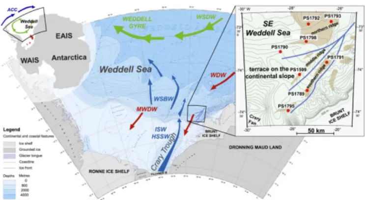
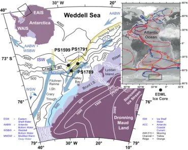
Figure 1.On the left side is an overview map showing whole Antarctica with the West (WAIS) and East (EAIS) Antarctic Ice Sheets as well as Antarctic Peninsula. The Weddell Sea (black square) is located in the southernmost part of Atlantic sector of the Southern Ocean. Additionally, the clockwise flowing Antarctic Circumpolar Current (ACC) and the Weddell Gyre (green arrows) are highlighted. The map in the centre shows a bathymetric chart of the Weddell Sea (Alfred Wegener Institute for Polar and Marine Research BCWS 1: 3 000 000; Bremerhaven, 1997).

Present-days flow direction of important water masses, i.e. High Salinity Shelf Water (HSSW), Ice Shelf Water (ISW), Weddell Sea Bottom Water (WSBW), Warm Deep Water (WDW) and the through heat loss Modified WDW (MWDW) are indicated (further information see chapter 2.2).

The core site area (black square) is located in the southeastern Weddell Sea close to the Brunt Ice Shelf. The small map on the right is a bathymetric map focussing on the southeastern Weddell Sea modified after (Weber et al., 1994) highlighting the Polarstern (PS) core sites referred to in this study (red dots). The core sites are located on ridges on a terrace of the continental slope.

Southeast of each ridge (brown colour) runs a channel. During the LGM the thermohaline current (blue lines) was flowing towards the NE in the channels. Due to the Coriolis force most of the transported sediment is deposited NW of each channel.

During the LGM and the last glacial transition while the East Antarctic Ice Sheet advanced to the shelf break, coastal polynyas were active above the continental slope, which induced brine rejection and therefore high-salinity water production (Weber et al. 2011). These dense water masses reworked sediment and drained into the channels, depositing the material mainly northwest of each channel because of the Coriolis force, building natural levees (Michels et al., 2002). Depending on seasonal velocity changes of the thermohaline current, the transporting sediment grain size changed, leading to varved sedimentation with alternating silty-rich and more

clayey layers. Bioturbated hemipelagic mud was deposited during times, when the ice sheet was retreated from the shelf edge and sea ice was reduced. The velocity of the thermohaline current is strongly decreased, leading to significantly lower linear sedimentation rates. The final East Antarctic Ice Sheet retreat was around 16 ka, marked by a transition from laminated to bioturbated sedimentation at every core site (Weber et al., 2011).

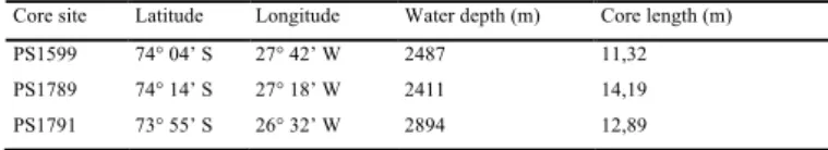
2 Study area and regional oceanography

We study gravity cores originating from the southeastern Weddell Sea, which were retrieved with R/V Polarstern (PS) in the late 1980s and early 1990s (Fig. 1). The core sites are located in channel-ridge systems on a terrace of the continental slope in 1900 – 3139 m water depth. Each ridge is up to 300 m high and up to 100 km long and runs parallel, on the northwestern side of a channel (e.g. Weber et al., 1994; Kuhn and Weber, 1993).

The Weddell Sea is the southernmost part of the Atlantic sector of the Southern Ocean.

The South Scotia Ridge marks the northern boundary and in the east it is limited by the Coats Land and Dronning Maud Land, where smaller ice shelves like the Brunt and Riiser-Larsen Ice Shelf are located offshore (Fig 1.). The southern Weddell Sea is covered by the Filchner-Rønne Ice Shelf. In the west the Antarctic Peninsula borders the Weddell Sea.

About 60 % (Orsi et al., 1999) to 70 % (Carmack and Foster, 1977) of the Antarctic Bottom Water (AABW) originates from the Weddell Sea, where Weddell Sea Bottom Waters (WSBW) is produced (Huhn et al., 2008; Foldvik et al., 2004). Maldonado et al. (2005) even argued that 80 % of AABW is produced in the Weddell Sea by brine rejection and supercooling.

Cyclonic movement of all water masses within the Weddell Gyre dominates the Weddell Sea circulation (Fig. 1). Relatively warm Circumpolar Deep Water (CDW) is transported by the Weddell Gyre from the Antarctic Circumpolar Current (ACC) southwards along the eastern boundary into the Weddell Sea and mixes with cold surface waters generating Warm Deep Water (WDW) (e.g. Orsi et al., 1993; Gordon et al., 2010). Through heat loss and mixing primarily during winter with Winter Water (WW) while flowing further to the West along the continental margin, WDW becomes Modified Warm Deep Water (MWDW). MWDW intrudes onto the shelf and mixes with the ISW to produce WSBW (Foldvik et al., 1985). HSSW is being generated during sea ice production by brine rejection (Foldvik et al., 2004; Petty et al., 2013) and is then supercooled by circulation under the ice shelf becoming dense Ice-Shelf Water (ISW; Nicholls et al., 2009). Passive tracer experiments also point to the Filchner-Rønne Ice Shelf as the main location for bottom water production (Beckmann et al., 1999).

Bottom-water drainage is across the over-deepened Filchner Trough along the south-north running channel-ridge systems into the Weddell Basin (Fig. 1). There, it is deflected to the left due to Coriolis Force and flows clockwise along the continental slope within the Weddell Gyre

(Foldvik, 1986). Although a current meter mooring (AWI-213) in the northeastern prolongation of the channel-ridge systems investigated here, still shows a near-bottom flow underneath the Weddell Gyre with a predominant northeastern direction (Weber et al., 1994).

3 Methods

Gravity core PS1795 was opened and splitted into archive and working halves at the laboratory of the Alfred Wegener Institute in Bremerhaven. All sampling was accomplished on working halves, while sediment physical properties were measured non-destructively at 1-cm increments on full round cores and archive halves. We used the GEOTEK Multi-Sensor-Core Logger (MSCL;

method see Weber et al. (1997)) for determining wet-bulk density (WBD), compression wave velocity (Vp) as well as magnetic susceptibility (MS). For MS measurements a Bartington point sensor (MS2F) was used and the data was volume-corrected. Also L*, a*, and b* colour components (Weber, 1998) were measured, using a Minolta spectrophotometer CM-2002. L*

gives information about the sediment lightness, colour a* reflects the amount of green-red, and colour b* is the blue-yellow component.

Water content was estimated on sediment samples every 5 cm by freeze-drying. Information about the geochemical composition was gained by analysing bulk samples with an element analyser.

Contents of total carbon (TC), inorganic carbon (TIC), and organic carbon (TOC; TIC subtracted from TC), as well as total nitrogen (TN) and total sulphur (TS) were measured. We also determined biogenic opal contents by leaching with 1M NaOH-solution according to the method see Müller and Schneider (1993). All resulting bulk data have been corrected for the containing amount of sea salt in the pore fluid (35 %_o).

To analyse sediment fabric, we cut out 1-cm thick, 10-cm wide, and 25-cm long plates from the centre of each core using a double-bladed saw. The plates were exposed for 3 to 5 minutes to a HP 43855 X-Ray System. After scanning the negatives at 300 dots per inch (dpi) resolution, we adjusted brightness and contrast to enable a better distinction of dark and bright layers, which are only a few millimetres thick.

Additionally we counted all grains >1 mm and >2 mm in diameter, reflecting ice-rafted debris (IRD). To do that, we used the scanned X-radiographs and place a semi-transparent 1x1 mm grid onto it; for further information on the method see Grobe (1987).

To obtain information on the distribution of chemical elements we measured the sediment cores non-destructively at 1-cm resolution using an Avaatech XRF core scanner (Jansen et al., 1998) at the Alfred Wegener Institute in Bremerhaven. For high-resolution element analysis, XRF- scanning was carried out every 0.2 mm on three consecutive split sediment core sections (197 – 499 cm) of PS1795 using a 3.0 kW Molybdenum tube. For these measurements, the ITRAX XRF- scanner (Cox Analytical, Sweden), a multi-function instrument for non-destructive optical,

radiographic, and chemical elemental sediment core analyses (Croudace et al., 2006), was used at the Cologne University laboratory. We also used the ITRAX scanner equipped with a 1.9 kW Chromium tube, to produce X-radiographs of the archive halves.

For accelerator mass spectrometry (AMS) radiocarbon dating we used well-preserved carbonate shell material originating from planktonic foraminifera Neogloboquadrina pachyderma (sinistral). Beforehand, H2O2 was added to each sample to remove the organic material. All measurements were conducted at the ETH laboratory of Ion Beam Physics in Zurich. AMS ¹⁴C ages were reservoir corrected (1.215 ± 30 years; see Weber et al. (2011)), based on age dating of carbonate shell material from a living bryozoa from neighbouring Site PS1418-1 (Melles, 1991).

Clam version 2.1 (Blaauw, 2010) and Marine09 calibration curve (Reimer et al., 2011) were applied to calibrate the AMS ¹⁴C of PS1795 and calculate calendar ages (Table 1). We used a cubic spline age-depth model with the weighted average of 10000 iterations with 95 % confidence range.

We also produced two overlapping thin sections (PS1795: 354.6-373.2 cm; 371.5-381.2 cm) for a detailed analysis of individual layers. Therefore, aluminium boxes were pressed into the sediment and then sliced with a fishing line. After carefully removing the sediment slabs from the core half, samples were immediately flash-freezed in liquid nitrogen and then freeze-dried. Slabs were then embedded in epoxy resin under vacuum and cured afterwards. For more details on the method see Cook et al. (2009) and Francus and Asikainen (2001). To obtain thin sections, the dried epoxy-impregnated sediment slabs were cut, grinded, and polished to a thickness of only a few millimetres. The thin sections were also scanned using the ITRAX system at the University of Cologne at 0.2-mm-resolution as well as scanned with a flatbed scanner for negative transparency scanning.

Additionally, we applied the RADIUS tool, providing rapid particle analysis of digital images by ultra-high resolution scanning of thin sections (Seelos and Sirocko, 2005), which uses the commercial image processing software analySIS (Soft Imaging System GmbH) controlled by three macro-scripts by Seelos (2004). Thin sections were therefore scanned on a fully-automatic polarization microscope in combination with a digital microscope camera at the University of Mainz. The scripts derive mineral-specific particle-size distributions that cover grain sizes from medium silt to coarse sand. The RADIUS tool was used on the thin sections (PS1795: 354.6-373.2 cm; 371.5-381.2 cm) at 100- m-resolution.

For automatic layer recognition and counting we used the BMPix and PEAK tool (Weber et al., 2010). First, grey values were extracted from the scanned X-radiographs using the BMPix tool. Then, the PEAK tool was used to count every maximum, i.e. bright layers, every minimum, i.e. dark layers, or every transition of the grey scale curve. For more precise counting results we manually examined and revised all counting results generated by the PEAK tool. See Sprenk et al.

(in review) for further information about the counting method, its uncertainties, and discrepancy estimations.

4 Results

4.1 Sediment-physical data

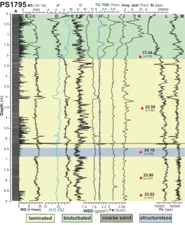
The 8.99 m long gravity core PS1795 (74°30'S, 28°11'W, 1884 meter water depth) is located southwest of the southern sediment ridge (Fig. 1). Sediments are relatively homogenous grey to brown (Fig. 2A), only the uppermost 23 cm are yellow to orange-brown due to oxidation.

Analyses of the coarse grain fraction (>63 m) of PS1795 every five centimetres shows that the main components of the coarse grains are quartz (80 % on average), but also feldspars, biotite, and hornblende make up 3 – 5 % each. Overall, maxima in MS (Fig. 2C) correlate with high high IRD counts (Fig. 2B).

From 2.15 m to the bottom of the core at 8.99 m, sediment is mostly laminated, consisting of alternating clayey and silty layers, each only up to a few millimetre thick. Laminated sediment consists mainly of terrigenous material with only 2 – 6 % biogenic opal, less than 0.2 % TIC/TOC, and about 0.04 % TN. WBD vary only slightly from 1.8 to 2.0 g/cm³. IRD content shows relatively strong fluctuations in the laminated sediment and varies between 0–18 grains/cm² (Fig.

2).

Between 6.42 – 6.87 m the sediment is nearly structureless, showing no bioturbation or laminations and contains only few IRD (Fig. 2B). Sediment-physical properties, e.g. MS, water content, and WBD of the 45-cm long section show only marginal fluctuations, suggesting a very homogenous composition.

A 3-cm thick coarse sand layer is intercalated into laminated sediment at 6.21 m, which is also reflected in sediment-physical properties. The coarse sand layer shows maxima in MS, IRD content, and WBD as well as minima in water content, TN, biogenic opal, Si, and Fe (Fig. 2).

The uppermost 2.15 m of PS1795 are characterized by highly bioturbated mud with varying IRD-content. The transition from laminated to bioturbated sediment is clearly documented in all parameters (Fig. 2). Water contents rise significantly from about 30 % to 40 %, colour a*

drops slightly, and WBD decreases to ~1.6 g/cm³. Overall, bioturbated sediment shows higher TOC, TIC, TN, and biogenic opal values than laminated sediment, indicating higher bioproductivity. Between 0.37 – 0.48 m bioturbated sediment contains high amount of IRD as well as the highest TOC contents and the lowest biogenic opal values.

Figure 2. Sediment-physical data from sediment core PS1795: A shows the red/green/blue (RGB) colour pattern; B shows the amounts of grains >1 mm, representing iceberg-rafted debris (IRD;

method see Grobe (1987)); C is magnetic susceptibility (MS) record; D is colour a* (green-red component); E shows the water content of the sediment; F gives lightness (L*); G is wet-bulk density (WBD); H to K are sea-salt corrected (sc) total organic and inorganic carbon (TIC/TOC), biogenic opal, and total Nitrogen (TN); L and M show chemical elements Silicon (Si), and Iron (Fe) determined with a X-ray fluorescence-scanner. AMS ¹⁴C ages (marked with red dots) measured on planktonic foraminifera Neogloboquadrina pachyderma are given in ka cal before present. The grey line at 2.15 m depth marks a possible hiatus (see chapter 4.2).

To form bioturbated sediment requires low sedimentation rates and at least partly open-water conditions (reduced sea-ice cover). Accordingly, bioturbated sediment was most likely deposited during times, when the ice sheet was retreated from the shelf edge (e.g. Weber et al., 1994; Weber et al., 2011). Therefore, the dense water masses are formed on the southern Weddell Sea shelf as today (see Oceanography chapter). Accordingly, due to the retreated ice sheet less ice-transported sediment was deposited on the upper slope.

4.2 Chronology

Using sediment slices up to 25-cm thick and labour-intense microscopic analysis, we managed to collect enough intact shell material from planktonic foraminifera Neogloboquadrina pachyderma for six AMS ¹⁴C analyses (Table 1). Three samples have less than 0.3 mg C, which is close to the detection limit of radiocarbon dating possible at ETH Zurich. Two of those samples show slight age reversals relative to those with greater amounts of C, and are therefore not included in the final age models. Nonetheless, the error range of AMS ¹⁴C age of 24.19 ± 0.29 ka at 6.68 m depth lies within the age range of the age-depth-models and is possibly caused by high linear sedimentation rates of about 1.1 – 1.6 m/kyr (Fig. 6).

We constructed two different age-depth-models for the sediment core PS1795. One age- model for undisturbed sedimentation relying only on the AMS ¹⁴C ages plus an age-depth-model, which includes a hiatus at a core depth of about 2.15 m. The X-radiograph highlights an erosive contact between laminated and bioturbated sediment at 2.15 m (Fig. 2) and also the varve counting results lead to the assumption that sedimentation is disturbed at the base of the bioturbated section.

However, it is not possible to count the varves accurately between 2.15 and 2.57 m due to the low quality of the X-radiographs, the material can be identified as varved sediment. Nonetheless, based on the visually detectable faint lamination, the material can be considered varves. Using an estimated LSR of approximately 1.1– 1.6 m/kyr the varved sediment possibly includes about 260- 380 varves, which gives an age for the top of the varved sediments between 21.8 and 22.4 ka. The topmost 2.15 m, cover about the last 17 – 18 kyrs as the AMS ¹⁴C age of 17.44 ± 0.36 ka close to the base of the bioturbated section reveals. This reflects linear sedimentation rates of only 0.12 m/kyr for the bioturbated sediment. Accordingly, the combination of varve counting and radiocarbon dating strongly suggests incomplete sedimentation, with a hiatus of approximately 3 to 4 kyr (Fig. 2).

Table 1. Accelerator mass spectrometry (AMS) ¹⁴C ages measured on planktonic foraminifera Neogloboquadrina pachyderma shells at the ETH laboratory of Ion Beam Physics in Zurich. Also the amount of C used for each measurement is included in the table. AMS ¹⁴C ages were reservoir corrected (1215 ± 30 years), based on age dating of carbonate shell material from a living bryozoa

from neighbouring Site PS1418-1 (Melles, 1991). Clam 2.1 (Blaauw, 2010) and the Marine09 calibration curve (Reimer et al., 2011) were used to calculate calendar years before present (cal yrs BP). For all ages also the estimated error of the dating method is given.

Laboratory code

Sample depth (cm)

Amount C (mg)

Uncalibrated

14C age (yrs BP) ± error

Age min (cal yrs BP)

Age max (cal yrs BP)

Probability (%)

ETH-48371 210-215 0,23* 15947 ± 77 17087 17797 95

ETH-48372 390-415 0,38* 22211 ± 86 24304 24946 95

ETH-48373 450 0,87 20501 ± 60 22221 22678 83.9

ETH-48373 450 0,87 20501 ± 60 22764 22950 8

ETH-48373 450 0,87 20501 ± 60 23140 23229 3.1

ETH-48374 655-680 0,31* 21912 ± 90 23903 24474 95

ETH-48375 775-795 0,42 21546 ± 80 23437 24170 95

ETH-48376 865-880 0,54 21643 ± 77 23558 24289 95

4.3 Varves

The varve character of the laminations has been established in earlier studies (Weber et al.

(1994, 2010a, 2011; Sprenk et al., in review). The most convincing argument is provided by core PS1789 (location see Fig. 1), which yields the visually most complete record of LGM varvation.

Two horizons at 199 cm and 1211 cm core depth date to 19,223 and 22,476 ka, respectively. Over this age difference of 3253 years (±529 years), we counted 3329 laminae couplets (see Fig. 8 of Weber et al., 2010) – a very convincing and robust indication of the seasonal nature of the lamination. The AMS ¹⁴C ages and varve counting results of PS1795 of this study also approve the seasonal sedimentation (see following chapters).

In this study, analyses concentrate on laminated sections of newly opened core PS1795.

Accordingly, the density of the coarser layers is slightly higher, leading to less darkening of the X- ray film (Axelsson, 1983), therefore X-radiographs have been successfully used for varve counting on sediment cores PS1599, PS1789, and PS1791 (Sprenk et al., in review). Although, the varved sections of PS1795 have similar average grain sizes as the cores studied previously, the seasonal differences are subdued, the X-radiographs do not show the differences accordingly (Fig. a) and the layers cannot always be adequately counted. To obtain more information on the texture and composition of the individual layers as well as to better understand the seasonal sedimentation process, we produced thin sections of the varved sediment.

4.3.1 Thin sections

Figure 4 shows that the scanned images of the thin sections provide more detailed information of the internal structure and composition of the varves. Strong thickness variations can be noticed both in the brown-coloured clayey layers and the light-coloured silty layers (Fig. 3), with thicknesses of only few hundred m up to 3 mm. There are only smaller variations in grain size and no erosional or sharp bases. Both findings argue against turbiditic deposition and favour varve formation (Fig. 3A). Sand and coarse-silt contents may vary significantly between individual layers. However, some parts of the record reveal very little difference in grain size so that individual layers are hardly recognisable in thin sections (Fig. 3) and cannot be distinguished on X-radiographs (Fig. 4) at all. Some layers are completely IRD-free (Fig. 3B), while others contain high amounts of sand-size grains (Fig. 3C). IRD appears to be mainly embedded in the lighter silty layers. Fig. 4D shows some large IRD – up to 2 mm in diameter – deforming the underlying layers. This is a clear indication that either icebergs or sea ice transported the IRD and deposited it by dropping onto the sea floor.

1 mm

1 mm 1 mm 1 mm

IRD

A

B C

D

Figure 3. Detailed images of a scanned thin section of PS1795. A gives an overview of the varved sediment and the thickness variation of silty (light-coloured) and clayey (brown-coloured) layers.

On the right side are three zoomed-in photos: Regular silty-clayey-layers (B); sand-rich silty layers with some ice-rafted debris (IRD) (C); D shows some individual large IRD, deposited by deforming the sediment below.

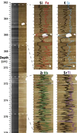
Figure 4. High-resolution element composition of a varved sediment section of core PS1795 (362 – 378 cm). The left side shows X-radiographs, generated using a X-ray fluorescence (XRF) scanner and scanned images of the thin sections. On the right side are zoomed-in images of the thin sections plus XRF-scanner element counts every 0.2 mm of the sediment slabs, from which the thin sections were produced.

4.3.2 Element composition

To investigate elemental composition changes, we scanned the sediment slabs prepared for thin sections (see Methods) every 0.2 mm (Fig. 4). Additionally, three archive halves were scanned for XRF at high resolution. Due to the fact that the varves are not exactly horizontally orientated and the radiographs, taken from a different part of the sediment as the XRF-scanner data were measured, both data sets do not reflect the same position in the sediment at the same depth.

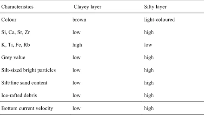
Therefore, we shifted the complete XRF-data curves a few millimetres (Fig. 5) in order to align them. Accordingly, most parts of Fig. 5 show a good correlation between XRF-derived elemental counts and the grey value curve estimated from X-radiographs, roughly reflecting density changes of the material. The most meaningful variation of elements in varved sediment are displayed in Figs. 4 and 5 and described in the following chapters. Characteristics of the clayey and silty layers are also highlighted in Table 2.

Si can either be of detrital or biogenic origin, i.e. bounded in biogenic opal (Sprenk et al., 2013). Given that the biogenic opal content of the glacial varves (Fig. 2K; chapter 4.1) of PS1795 is less than 5 %, with a mean of 2.2 %, Si is mostly of detrital origin. Analyses of the coarse- grained fraction also revealed that, on average, about 80 % of the particles coarser than 63 m are actually quartz grains. The combination of thin sections and XRF-data (Fig. 4) highlights that Si counts are relatively enriched in coarser, light-coloured layers relative to brownish clayey layers.

This indicates that Si counts every 0.2 mm can be an ideal additional tool for detrital varve counting. Figure 5 shows that the overall amount of Si also correlates to grey values derived from radiographs, which are positively correlated to sediment density (see methods). Si counts are also a good indicator for facies changes (see Fig. 2). Si counts are significantly lower in bioturbated sections relative to varved sections, due to increased water content of the sediment.

Potassium (K), iron (Fe), and titanium (Ti) show strong positive correlation, which is reflected in the Ti/Fe ratio of r²=0.84 and K/Ti ratio of r²=0.90. This suggests that K, Fe, and Ti are mainly bounded in clay minerals such as the chlorite and illite groups as well as mica biotite.

Figure 4 highlights that K, Fe, and Ti show maxima in brownish coloured clayey layers.

Rubidium (Rb) has a similar ionic radius as K. Therefore, it commonly replaces it and can often be detected in K-feldspars, mica, and clay minerals (Chang et al., in press). Cu, Zn, Rb, Cs, Ba, and Sn are generally related to clay minerals (Vital and Stattegger, 2000). Fine-grained sediments show typically high Rb counts (Dypvik and Harris, 2001), which is also documented in varved sections of PS1795, where Rb is like K, Fe, and Ti enriched in clayey layers (Fig. 4).

Strontium (Sr) has an atomic radius similar to calcium (Ca) and can therefore replace it easily. Both elements are slightly enriched in siltier layers (Fig. 4). Ca and Si show a good correlation with a coefficient of r²=0.78.

Zirconium (Zr) is comparatively immobile, mainly residing in heavy minerals, e.g. zircon, resistant to chemical as well as physical weathering (Wayne Nesbitt and Markovics, 1997; Alfonso

et al., 2006). Thus Zr is mainly transported with coarser particles (Vogel et al., 2010). Zr shows maxima mainly in coarser silty layers. Comparing the scanned thin sections and the Zr counts (Fig.

4), reveals that especially thicker and coarser silty layers have maxima in Zr counts.

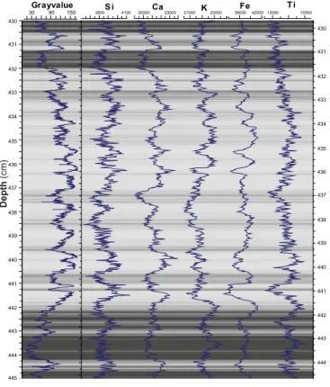
Figure 5. Seasonal-scale changes in chemical element composition: high-resolution X-ray fluorescence scanner data (area counts) every 0.2 mm of PS1795 core section (430 – 445 cm).

Additionally, the estimated grey scale value curve estimated from scanned X-radiograph using the BMPix tool (Weber et al., 2010) was added.

4.3.3 RADIUS tool

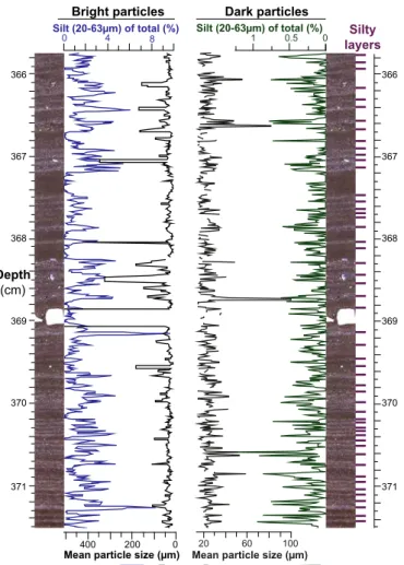
To gain more information on the particles and their size distribution in varved layers, we applied the particle analysing RADIUS tool (Seelos, 2004) on high-resolution, scanned thin sections. The RADIUS tool differentiates between (i) bright particles, i.e. mainly quartz, and light feldspars, (ii) dark particles, i.e. opaque minerals, and (iii) carbonates (Seelos and Sirocko, 2005).

Carbonate particles are neglected in Fig. 6 given that the values are extremely low and not significant, which is also reflected in the low TIC content of varved sediment (Fig. 2).

Figure 6 shows the percentage of detected bright and dark particles in the grain size fraction 20 – 63 m, i.e. medium to coarse silt, of total grains (i.e. of all classified grains up to 200 m in diameter). In lighter layers, bright silt-sized particles have local maxima and are accounting for up to 10 % of the total grains. Also, the mean size of the bright particles is mostly higher in lighter layers than in brown layers (Fig. 6). Although, single IRD, e.g. at 385.5 or 369 cm, strongly influence the mean particle size. The median size of bright particles is about 34 m. In contrast to that, dark particles have only median sizes of about 22 m. This is also reflected in the overall low content of dark particles in the medium to coarse silt fraction with only up to 1.2 % of all classified grains and yet in some parts even no detected dark particles. The correlation of the silt-sized dark particles and the sediment layers is not as striking as for the bright particles (Fig. 6). However, many lighter layers also show increased amounts in silt-sized as well as higher mean size of dark particles.

5 Discussion

5.1 Seasonal sedimentation changes

Our age model relying on AMS ¹⁴C dates and varve counting reveals that the varved sediment was deposited during the LGM, when the ice sheets in the Weddell Sea area had most likely advanced to the shelf break (e.g. Weber et al., 2011; Hillenbrand et al., 2012). The estimated linear sedimentation rate of about 1.1 – 1.6 m/kyrs for the varved sediment of PS1795 (e.g. Fig. 6), is somewhat lower than established for core sites farther downslope on the same channel-ridge system. Sprenk et al. (in review) calculated mean linear sedimentation rates from varve counting varying between 2.2 and 5.3 m/kyr for the cores PS1599, PS1789, and PS1791 (Fig. 1). The differences in sedimentation rates are possibly related to the location of the core sites. In contrast to the earlier investigated core sites located on the sediment ridges NW of the channels, PS1795 originates from a shallower position farther southwest outside the channel, on a steeper part of the continental slope (Fig. 1) where the channel-ridge system starts to develop.

Figure 6. Detailed particle analysis of the varved sediment section 365.8-371.5 cm with the RADIUS tool (Seelos and Sirocko, 2005) applied on high-resolution scans of the thin sections.

Total refers to all analysed particles up to 200 m size. Purple bars mark the 52 counted light- coloured silty layers with a resultant linear sedimentation rate of about 1.1 m/kyrs.