Dynamics and Structure of Complex Networks

(1)

Dynamics and Structure of Complex Networks

Inaugural-Dissertation

zur Erlangung des Doktorgrades der Mathematisch-Naturwissenschaftlichen Fakult¨at

der Universit¨at zu K¨oln

vorgelegt von

Steffen Karalus

aus Bad Soden-Salm¨unster

K¨ oln 2015

(2)

Prof. Dr. Johannes Berg

Tag der m¨undlichen Pr¨ufung: 22. Oktober 2015

(3)

Kurzzusammenfassung

Diese Arbeit untersucht die Beziehung zwischen strukturellen Eigen- schaften und dem Verhalten von dynamischen Prozessen in komplexen Netzwerken. Aufbauend auf Ideen aus der biologischen Evolution oder Monte Carlo-Simulationen wird die Methode der Netzwerk- evolution entwickelt. Sie dient zur Generierung von Netzwerken mit vorgegebenem dynamischen Verhalten ohne explizite Vorkenntnis, wie strukturelle Eigenschaften die Dynamik beeinflussen. Insbesondere werden Laplace-Dynamiken als Klasse von grundlegenden – einfachen jedoch hochgradig relevanten – Prozessen betrachtet. Ziel der Evolution ist ein Potenzgesetz im Spektrum der Laplace-Matrix, das die spektrale Dimension als charakteristische Größe für die Beschreibung von Diffusionsprozessen definiert. Die erfolgreich evolvierten Netzwerke weisen heterogene Strukturen, bestehend aus dicht verbundenen Kernen und dünnen Randbereichen, auf. Durch Rekonstruktion der evolvierten Netzwerke wird der Einfluss von Gradverteilung und Grad- Korrelationen auf die spektralen Eigenschaften untersucht. Hierfür werden Zufallsnetzwerke mit der Gradverteilung und den Grad- Korrelationen der evolvierten Netzwerke generiert und die Laplace- Spektren verglichen. Schließlich werden homogene Netzwerke mit dem vorgegebenen Potenzgesetz im Laplace-Spektrum durch Beschränkung der Evolution auf reguläre Netzwerke erzeugt. Die so evolvierten Netzwerke sind gekennzeichnet durch gehäuft auftretende symmetri- sche Motive. Dies wird für ein systematisches Coarse-Graining der Netzwerkstrukturen genutzt. Dadurch lassen sich die Laplace-Spektren eindeutig in Beiträge der symmetrischen Motive einerseits und der unterliegenden großskaligen Strukturen andererseits aufspalten.

(4)

(5)

Abstract

In this thesis the relationship between the structure of complex networks and the behavior of dynamical processes on these networks is studied by network evolution. Adopting ideas from biological evolution or Monte Carlo simulations the method of network evolution is developed as strategy to generate networks with a prescribed dynamical behavior without any prior knowledge about the structure- dynamics relation. Here, Laplacian dynamics are considered forming a basic—simple but highly relevant—class of dynamics. Networks are successfully evolved towards a power-law scaling in the spectrum of the graph Laplacian which defines the spectral dimension as important characteristic of diffusion behavior. The resulting evolved networks exhibit heterogeneous structures with densely connected cores and sparse peripheries. The influence of the degree distribution and degree correlations on the spectral behavior is investigated. To this end random networks with the degree distribution and degree correlations of the evolved networks are generated and the Laplacian spectra are compared. Finally, homogeneous networks with the prescribed power law in the Laplacian spectrum are generated by restricting the evolution to regular networks. The resulting evolved networks are found to be highly symmetric. The symmetry is exploited to construct quotient networks as systematic coarse-graining separating the Laplacian spectra into contributions from the repeating symmetric motifs on small scales and the underlying large-scale structures, which are particularly relevant in determining the spectral dimension.

(6)

(7)

List of Figures

1.1. Illustration of a neural network . . . 17

1.2. The structure of the Internet . . . 18

1.3. Zachary’s karate club network . . . 20

3.1. Network topology of the finite Sierpinski triangle of generation 6. . . 52

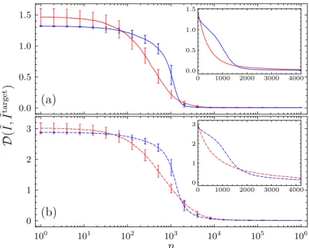
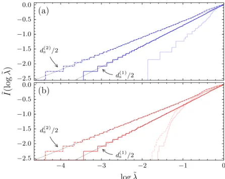
3.2. Change of spectral distanceD( ˜I,I˜^target) with evolutionary time steps n . 53 3.3. Logarithmically integrated eigenvalue densities ˜I(log ˜λ) before and after the evolutionary optimization . . . 55

3.4. Average return probabilityP₀(t) for initial and evolved networks . . . 56

3.5. Degree distributions P(k) of initial and corresponding evolved networks . 56 3.6. Evolution of degree assortativityr and clustering coefficient C . . . 57

3.7. Typical network configurations taken from the evolutionary optimization . 59 4.1. Histogram of spectral distances in individually reconstructed networks . . 63

4.2. Averaged logarithmically integrated Laplacian spectral density of reconstructed networks . . . 64

4.3. Typical network configurations taken from the individual reconstruction . 65 4.4. Histogram of spectral distances for the reconstruction from independently averaged correlations . . . 66

4.5. Distributions of number of connected components and average spectral distances by number of components . . . 67

4.6. Typical network configurations reconstructed from independently averaged distributions . . . 68

4.7. Reconstruction averages of evolutionary time series . . . 69

5.1. Schematic of the edge-crossing update . . . 72

5.2. Typical configurations of k-regular networks evolved towards a target spectral dimension of d⁽¹⁾_s = 1.4 . . . 73

5.3. Redundant Laplacian eigenvectors of the most prominent motifs in evolved networks . . . 78

5.4. Illustration of the coarse-graining procedure . . . 78

5.5. Logarithmically integrated Laplacian eigenvalue densities of evolved networks together with quotients and s-quotients . . . 80

5.6. Typical 3-regular evolved network and corresponding s-quotient for target spectral dimension d⁽²⁾s = 1.1 . . . 81

5.7. Histogram of linear segment lengthssin s-quotients . . . 82

(10)

(11)

List of Tables

3.1. Spectral distances Dini before andDfin after the evolutionary optimization 54 5.1. The coarse-graining in numbers . . . 79

(12)

(13)

Symbols

N Number of vertices in a network.

M Number of edges in a network.

A_ij Elements of the adjacency matrix.

L_ij Elements of the graph Laplacian.

k_i Degree of vertex i, the number of edges connected to it.

P(k) Degree distribution, the probability that a randomly chosen vertex has degree k.

P_e(k) Edge end distribution, the probability that a vertex at the end of a randomly chosen edge has degree k.

P(j, k) Joint degree distribution, the probability that a randomly chosen edge connects vertices of with degreesj andk.

r Assortativity coefficient measuring the degree-degree correlations.

C Global clustering coefficient measuring the overall transitivity.

Ci Local clustering coefficient measuring the transitivity at vertexi.

C(k) Degree-dependent clustering coefficient measuring the transitivity of vertices in the degree class k.

P0(t) Average return probability, probability that a random walker is located at its origin at time t, averaged over all starting vertices.

I(λ) Integrated Laplacian eigenvalue density.

d_s Spectral dimension, describing the scaling of the Laplacian spectral density.

D( ˜I,I˜⁰) Spectral distance between the two logarithmically integrated densities ˜I and ˜I⁰.

(14)

(15)

1. Introduction

Everything is simple and neat—except, of course, the world.

Goldenfeld and Kadanoff

Complex Systems

Undoubtedly, the world we are living in with the phenomena we are observing and, not only as physicists, trying to understand is a complex world. It consists of a vast amount of entities of extremely different sizes, masses, and many other properties with an even larger number of interactions between them. Describing the whole complexity of this world would not only be cumbersome but is truly impossible.—To mention just two reasons for this, consider the fact that we will never be able attain full information about the state of each and every atom in the universe due to quantum mechanical uncertainty and the relativistic event horizon. Additionally, and in a certain sense more fundamentally, the device to describe the world would have to be part of and interacting with the rest of the world, leaving us without any material to store information and perform computations.—The sciences in general and in particular physics have made much progress in the description and the understanding of the world by the use of reductionism. The idea to separate the essential aspects from the less important has led to the discovery of again and again more elementary entities and more fundamental interactions. The importance of these discoveries like quantum mechanics and elementary particle physics as well as general relativity and cosmology is, of course, beyond any doubt. Nevertheless, it is a naive fallacy to conclude that other fields of science can be simply deduced from more the fundamental ones. The emergence of collective phenomena and the shifts in which aspects are considered as essential, depending on the level of description, are subsumed in the manifestation “More Is Different” by Anderson (1972):

The behavior of large and complex aggregates of elementary particles, it turns out, is not to be understood in terms of a simple extrapolation of the properties of a few particles. Instead, at each level of complexity entirely new properties appear, and the understanding of the new behaviors requires research which I think is as fundamental in its nature as any other.

In this hierarchy of science the elementary entities of one level of description are governed by the laws of the more fundamental level, but in the transition from one to the other a completely new field emerges. These transitions are studied in statistical physics and complex systems science. The basic entities of a system and their local interactions

(16)

are considered to be known. From the non-trivial interplay of many of those entities, however, the complexity of the new field arises.

But what actually is complexity? A strict definition of which systems and phenomena are considered as “complex” and which as “simple” does not exist so far. However, there seems to be an agreement on a number of aspects a complex system has. The emergence of collective phenomena as a central feature of complex systems was already mentioned above. On the level of observations important features are structure formation and intermittency or “structure with variations” (Goldenfeld and Kadanoff, 1999). Also self- organization is considered as an important feature of many complex systems. This idea was very successfully driven forward in the concept of self-organized criticality (Bak et al., 1987). In a systematic analysis, Chu et al. (2003) reason that necessary features of complexity are internal inhomogeneity, adaptivity of agents, nonlinear interactions, and a net-like causal structure as well as radical openness and contextuality. While the first four form the constituents ofcomplex adaptive systems which can be described byagent-based models they conclude that together with the latter two a general unified theory of complexity might not be possible to achieve. For the study of complex systems, Amaral and Ottino (2004) consider nonlinear dynamics, statistical physics, and network theory as the most important tools. Out of these three, network theory is the youngest and most rapidly developing field. As an integral component of complex systems it has become a very active research topic over the last fifteen years.

Networks

A network model describes binary relations between elements of a discrete set of entities.

This includes traditional arrangements such as regular lattices (as studied, e.g., in solid state physics), all-to-all or randomly chosen interactions as well as more complex structures with very distinct features. Since interactions in many natural, technological, or socio-economic systems are indeed pairwise, or can at least be approximated as such, networks provide a quite general description of interaction patterns. In the following, some important examples of systems which were successfully modeled as networks are presented. More detailed information on these systems and references can be found in several review articles (Albert and Barab´asi, 2002; Dorogovtsev and Mendes, 2002;

Newman, 2003b) and a book (Newman, 2010).

In biology, a number of systems over all relevant length scales can be usefully represented as networks. On the sub-cellular level,protein-protein interaction networks describe the interactions between different proteins in a biological cell. Two types of proteins are connected in this description if they can, in their native folded state, interlock to form protein complexes. These interactions primarily do not involve chemical reactions. In a metabolic network the pathways of cell metabolism are recorded, i.e., the chemical substances and their reactions involved in the process of breaking down nutrients and making energy and useful biomolecules available for the functioning of the cell. This is an example of a system which is most effectively modeled as a directed network. In order to have well defined metabolic pathways the chemical reactions are

(17)

Figure 1.1. Illustration of a neural network. Shown is a network of nerve cells from the chick cerebellum in an original drawing by the Nobel laureate Santiago Ram´on y Cajal.

(Ram´on y Cajal, Estructura de los centros nerviosos de las aves, Madrid, 1905)

best described by asymmetric relations between the different metabolites. The same holds true for gene regulation networks describing how the expression of different genes in a cell regulate each other. If a certain gene is expressed, i.e., DNA is transcribed into messenger RNA which is then translated into gene products such as proteins, its products may promote (excitatory interaction) or suppress (inhibitory interaction) the expression of other genes building up a complex regulatory system. Similar regulatory mechanisms with excitatory and inhibitory connections which are, however, of completely different origin are found in neural networks. They consist of specialized excitable nerve cells, so-called neurons, which are electrically connected by synapses or gap junctions. While there are about 10¹¹neurons found in a human brain the neural network of the nematode wormCaenorhabditis elegansconsist of only 302 neurons making it an ideal model system which has been very well studied. A historic illustration of a neural network in the cerebellum of a chick is displayed in figure 1.1. On the scale of a whole organism,vascular networks describe the connectivity structure of blood vessels or equivalent transport systems in plants. Physiological networks are used as models for the interactions of different organs of the human body. On even larger, ecological scales food websdescribe the hunting relations between different species in an ecosystem. As predator-prey relation are in general asymmetric, these are also most naturally modeled as directed networks.

There is also a number of technological systems which can be very effectively described as networks. Although these systems are man-made they are often not completely under control of a central organization unit and exhibit features of complex systems. A very famous and well-studied example is theInternet, a network of physical data connections between computers and other telecommunication devices such as routers. It has no

(18)

Figure 1.2. The structure of the Internet as connections between the “class A subnets”, groups of computers with similar IP addresses, in 2003. The connections indicate the observed routes taken by data packages sent through the Internet and the colors indicate different groups of domain names. (Image: The Opte Project / Barrett Lyon)

(19)

superordinated organization or central authority and there is no “official map” of the Internet. Instead, its topology has to be explored by experimental measurement just like in any natural system. Figure 1.2 shows the connectivity structure of the Internet derived from such a measurement. Not to be confused with the Internet must be the World Wide Web, a network of web pages connecting to one another via hyperlinks without any physical structure. Just as in the case of the Internet, the structure of the World Wide Web has to be measured experimentally. Another class of network systems our daily live depends on crucially are supply networks like power grids and the supply infrastructure for gas, water, oil, etc. In this context, mostly the large- scale distribution networks such as the high-voltage transmission lines for the long- distance transport of electrical energy are considered. These grids are usually managed and supervised by single authorities and complete maps are available. In this case, determining the topology is not a difficult task. Nevertheless, also power grids show complex structures and sometimes counterintuitive behavior. Finally in the group of technological systems,transportation networksform a very important part of our modern infrastructure. Obviously, roads and railway lines form networks connecting cities and railway stations. Although these networks are restricted to exist on a plane (except for tunnels and bridges) they exhibit complex structures. Networks of airplane or ship connections, on the other hand, are not that strictly bound to any man-made connecting infrastructure.

A third realm in which network models are applied are the social and economic sciences. For most people the term might be associated with online social networking platforms like Facebook but the notion of a social network was introduced long before the Internet even existed. In fact, sociology may actually have the longest tradition in quantitative, empirical work on network systems. The concept of sociograms—a network representation of social relations in a group—even dates back to the 1930s (Moreno, 1934). In general, a social network describes a set of people and some relation like friendship, partnership, sexual contacts, or professional relations between them. The size of such networks may range from small groups like the 34 members of a karate club (one of the most famous examples in the literature, the network structure is shown in figure 1.3) to possibly all human beings on the earth. The collection of data for these networks by traditional methods like interviews and questionnaires was quite cumbersome and restricted to smaller communities. Today, much larger datasets exist—but might not be publicly accessible—for online networking platforms. A special case of social networks are collaboration networks recording the participation of people in joint projects like actors appearing in the same movie or scientists co-authoring an article. Large datasets for these networks can be extracted from online databases such as the Internet Movie Database or the Web of Science. By means of the latter, also citation networks can be recorded, describing the citation relations between scientific publications. These relations are strictly directed, mutual relations are (almost) impossible since only previously published articles can be cited. In economic sciences, networks of business relations are studied. These might bebanking networksdescribing interbank lending and therefore interdependencies of banks. In the study of markets, trading networks record trade relationships between companies, states, or whole economic zones.

(20)

2

1 3 4

5 6

7 8

9 10

11

12

13 14

17

18 20 22

26

24 25

28 29

30

27

31 32

33

15 16 19 21 23

34

Figure 1.3. Zachary’s karate club network. A network of friendship between the 34 members of a university karate club, recorded by Zachary (1977). By analyzing the structure of the network, Zachary was able to predict how the club divided in two groups, which was observed later on in a conflict between the instructor (number 1) and the administrator (number 34) of the club.

The various systems mentioned here are of completely different nature. The constituent elements and also the represented relations of one example might have nothing in common with those of another one. Most of the systems vary substantially in their sizes, in the way they formed, and how they evolve. However, if one solely focuses on the network representation and forgets about what this abstraction stands for some reappearing structural properties shared among many of those systems can be uncovered. This observation triggered the general interest in networks by themselves as objects of scientific studies. The hope to discover universal properties of networked systems is what made them especially interesting from the view of theoretical physics. In the most simple description, a network consists of a set of points connected by lines. In mathematical terms the points are referred to asvertices, the lines are callededges, and together they form a graph. The number of edges that are connected to a given vertex is called itsdegree. One observation in many networks is a rather broad distribution of the vertex degrees. This means that most elements have just a few connections while a small but significant number of elements have extremely many, the so-called “hubs”.

Specifically, such heavy tails are found if the degree distribution follows a power law.

In this case, the network is often referred to as ascale-free network. Although already observed in the 1960s in the context of citation networks (de Solla Price, 1965), the phenomenon was popularized more recently by Barab´asi and Albert (1999). Another intriguing characteristic of many network systems is thesmall-world effect. The distance between two vertices in a network can be defined by the minimum number of edges that have to be traversed in order to reach one vertex from the other, the so-called geodesic distance. It has been observed that the mean geodesic distance between vertex pairs in many networks is surprisingly small, the networks form a “small world”. This has been popularized as the “six degrees of separation” referring to the average number of

(21)

acquaintance connections necessary to link two randomly chosen people in the United States of America (Milgram, 1967). Although it might sound peculiar at first, the small-world property alone is also found in random networks, even in the most simple random graph models, the famous Erd˝os-R´enyi networks (Erd˝os and R´enyi, 1959).

Only together with a high level of clustering, the tendency to find groups of densely interconnected vertices, it becomes a non-trivial and astonishing characteristic of many empirical networks. This has been addressed in a seminal work by Watts and Strogatz (1998), a second foundation of modern network theory.

Network Dynamics

Why do people study networks and complex systems? By themselves the complex structures found in real-world network systems might appear fascinating but in the end it is the understanding of how these systems function that drives the interest in network research. In most of the systems described above the pattern described by the network actually serves as substrate for a dynamical process taking place on top of it, one sometimes speaks ofdynamics on networks. Each vertex in the network stands for a dynamical variable and edges describe which variables are influenced by the dynamical state of which other variables. In gene regulation networks, the vertices stand for the different genes and the dynamical variables are their expression levels. The expression of a certain gene dynamically regulates the expression of all other genes connected to it by an edge. Similarly, the dynamics of neural networks may be viewed. The neurons form the vertices of the network and their activities are the dynamical variables regulating each other via the synaptic connections. In food webs, the number of individuals of certain species is described by dynamical variables that change due the foraging interactions.

A slightly different point of view can also be taken by considering the distribution of biomass as dynamical quantity and the network as describing its flow through the ecosystem. In supply networks, usually a single commodity has to be transported from sources to sinks. One can simply consider the amount of the commodity at a vertex as dynamical variable. This might, however, not be enough if more complicated processes are imposed by the special system. In AC power grids, for example, the voltage oscillations govern the dynamics of the whole system and Kirchhoff’s laws have to be satisfied. In contrast to the single commodity case, in a transportation network different objects need to be transported to their individual targets. In this case, their individual positions in the network might be a better choice of dynamical variables. The Internet can also be considered as a transport network for data packages which are sent from one computer to another. On social networks, a large variety of dynamical processes is taking place which can be considered separately or in combination. Of high practical importance are epidemic spreading dynamics describing how infectious diseases spread from individual to individual through personal contacts. Also the spread of information, of fads, or of innovations in a society are dynamical processes on social networks. The term “viral phenomenon” has been adapted from epidemic spreading for these processes,

(22)

if the piece of information, the fad, or the innovation is passed on from one individual to the next without a central broadcaster, just like a contagious disease.

The local dynamical rules—the internal dynamics of an isolated node as well as the couplings—of these systems obviously differ a lot. Nevertheless, they share an important feature putting them in the focus of dynamical network research. Namely, their internal dynamical rules and local coupling can be considered as rather “simple”. The complex dynamics of a system as a whole arise from the way they are coupled, i.e., the network structure. Concerning the practical question of how the dynamics of such a system can be controlled or at least influenced, often not much can be done about the local dynamics.

Instead, the important question is how the network structure has to be altered in order to change (or preserve) the overall dynamics. In the case of epidemic spreading dynamics, for example, one might want to know which individuals should be removed from the process by vaccination in order to efficiently prevent the disease from spreading over the whole population. In the case of the Internet or other infrastructure networks usually the opposite case is desired, how can the whole system be kept running if some parts of it fail.

A second dynamical aspect of networks is the evolution of network structure, sometimes called dynamics “of” networks to distinguish it from the dynamics “on”

networks mentioned above. An evolving network changes its structure in the course of time, i.e., vertices or edges are added to or removed from the network. Again, almost all of the exemplary systems mentioned above are actually evolving their structure in time.

The technological networks are often expanded to increase their capacity or downsized to make them more cost efficient. Frequently, new computers are added to the Internet and others are removed, new websites appear and old ones are deleted from the servers of the World Wide Web, new streets and railways are built, new airline connections are established while others are closed down, old power plants are replaced by new ones.

Also social networks are constantly changing, people die and others are born, every day we meet different people and new technological developments or changing habits allow us to interact with other people. In biological networks, biological evolution is one ubiquitous source of changes in the constituents and interaction patterns. Especially on molecular scales, genetic mutations can directly change protein sequences and therefore their structure and interactions with other proteins or modify the metabolic pathways of certain substances and, by this, the ability of an organism to make use of different nutrients. Additionally, there may exist other sources of structural changes in biological networks like the brain plasticity in neural networks or the invasion of alien species into an ecosystem.

In the case when both kinds of dynamics, dynamics on a network and network evolution, are to be considered, the typical time scales of the two processes become important. They may either be of the same order of magnitude meaning that the dynamical variables of the process change their state more or less at the same rate as the network structure is modified. In this case, one speaks of coevolutionary or adaptive networks (Gross and Blasius, 2008) since the network structure can adapt to the state of the dynamical variables. Or the two time scales are well separated meaning that the dynamical variables change many times and probably have enough time to reach an

(23)

attractor until the network structure changes. In this case it is reasonable to assume that the evolution “sees” the overall behavior or performance of the dynamical process instead of a single dynamical state. This is certainly the case in biological evolution where, for example, gene expression levels change many, many times during the lifetime of an organism until mutations might occur from one generation to the next. Also the dynamics of neuronal activity is much faster than the formation of synaptic connections.

In most technological networks a similar situation is found. Data packages are sent through the Internet much faster than new computers are installed, trains and cars run faster than new streets or railways are built, and voltage oscillations in a power grid have obviously a higher frequency than the construction of new power plants and transmission lines. In social networks, the situation can be different. It is very likely that people change their behavior and the way they interact with other people when they become infected by a disease or when they change their political opinion. In these cases the interaction network adapts to the current dynamical state. A different situation might have to be considered on other scales of human interaction. To describe the global spreading of some disease one might use airports as network vertices and consider them as infected if a certain threshold of people in the city or region carry the infection. In this case, the airline connectivity will usually not adapt to the dynamical state and time scales are well separated again.

In this thesis, the relation between network structure and the global behavior of dynamical processes is studied. The focus lies on Laplacian dynamics, an important class of processes in which the time evolution is governed by the graph Laplacian operator. This class comprises very basic but highly relevant processes such as diffusion and random walks or synchronization of oscillators with many significant applications.

Inspired by the evolution of dynamical networks under a separation of time scales, a method of evolutionary optimization of network structure for a prescribed global dynamical behavior is developed. The overall dynamical behavior is characterized by the eigenvalue spectrum of the graph Laplacian bridging between network structure and dynamics. By this, the dynamics do not have to be carried out explicitly.

Related ideas were applied before in studies on optimal or pessimal network structures for the synchronizability of oscillator systems (Donetti et al., 2005, 2006, 2008) and reconstruction of networks from their Laplacian spectra (Comellas and Diaz-Lopez, 2008;

Ipsen and Mikhailov, 2002).

Thesis Outline

The remainder of this thesis is structured as follows. Chapter 2 introduces the mathematical concepts and tools for the description of complex networks. Observables to quantify topological characteristics are covered as well as random network models reproducing different structural properties. An overview of dynamical processes on networks is given with a focus on diffusion and random walks. Finally, the graph Laplacian as generator of an important class of dynamics is introduced together with its relation to structural and dynamical network properties. In chapter 3 the method of

(24)

evolutionary optimization of network structure for anomalous diffusion described by the spectral dimension is developed. The technique is successfully applied and the resulting network structures are analyzed. Chapter 4 investigates the influence of structural correlations on the dynamical behavior in the evolved networks. To this end, random networks are generated having the same correlation functions as the evolved networks and their Laplacian spectra are compared. In chapter 5 the evolutionary optimization is further restricted to find networks which are homogeneous in their local connectivity.

The resulting evolved networks exhibit a high level of structural symmetry which is exploited in a systematic coarse-graining to find the underlying backbone structures and their relevance for the anomalous diffusion behavior. Chapter 6 summarizes the results of this thesis and discusses its findings. In the appendix, the algorithm applied for the random network generation is explained in detail and the numerical libraries which were used are listed.

(25)

2. Dynamical Networks

In this chapter, the mathematical concepts for the quantitative description of networks and their dynamics are introduced. The corresponding mathematical field is graph theory. Since this is a large field with a long history, only the concepts and results that are necessary for the understanding of this thesis are covered. More extensive information about the presented concepts and additional topics can be found in the literature (e.g. Barrat et al., 2008; Newman, 2010).

2.1. The Structure of Complex Networks

A network, as already introduced above, consists of a set of basic entities and a collection of pairwise connections between them. In the language of graph theory the basic entities are called vertices or nodes. The connections are described as pairs of vertices and are called edges orlinks. Together, the vertex set V and the corresponding edge set E form a graph G = {V,E}. Two vertices that are connected by an edge are called adjacent or neighboring. Some authors distinguish between networks as objects of empirical observations and graphs as strictly mathematical concepts that can be models for these “real-world” networks. In this thesis, as in most physical literature, no such differentiation is made, the terms “graph” and “network” are used interchangeably.

Several cases, or types of networks, have to be distinguished. The edges may be either directed or undirected, so that the edge set consists of either ordered or unordered pairs of vertices. In the former case, one speaks of adirected network ordirected graph, shortly calleddigraph. Secondly, it may be allowed or forbidden to havemultiedges(several edges between the same pair of vertices) so that the edge set contains an element more than once. Thirdly, it may be allowed or forbidden to have edges from a vertex to itself, so- calledself-edges orself-loops. An undirected network which contains neither multiedges nor self-loops is referred to as asimple network.

2.1.1. Formal Description

Vertex and edge sets provide the defining representation of networks. There exist, however, a number of equivalent ways to describe a network formally. The vertices are most easily identified by their position in the vertex set, which can then be simply written asV ={1, . . . , N}whereN =|V|denotes the number of vertices in the network.

In physics, N is called the size of the network although in graph theory the “size” of the graph is |E|, the number of edges, whereas |V| is called the “order” of the graph. An edge between verticesiandjis then denoted as the pair (i, j), the edge is calledincident to i and to j. The edge set is then the list of pairs E = {(i₁, j₁), . . . ,(i_M, j_M)} where

(26)

M = |E| is the total number of edges in the network. Such edge lists are sometimes used to represent a network on a computer. For most computational purposes, however, the adjacency list representation is more efficient. It associates with each vertex a list of all its adjacent vertices. In a directed network, only the outgoing or only the incoming connections are considered in the adjacency list. For analytical calculations, it is usually more convenient to work with matrices rather than with lists. The basic matrix representation of a network is the adjacency matrix A. For a network with N vertices it is aN ×N square matrix with elements

A_ij =

(1 if there is an edge between vertices iand j,

0 otherwise. (2.1)

The adjacency matrix of an undirected network is symmetric, A_ij =A_ji. For directed networks, it has to be specified whetherA_ij relates to an edge from i toj or from j to i. Both conventions are found in the literature and often the authors do not explicitly specify which definition they use. In this thesis,A_ij in a directed network will stand for edges fromi toj, i→j. Also networks with multiedges and self-loops can be uniquely described by an adjacency matrix. For this, A_ij simply has to be generalized to be the number of edges between the verticesi and j. A self-loop in an undirected network is most practically described by setting the corresponding diagonal element A_ii = 2, or A_ii= 2nin the case ofnself-loops at vertexi. This definition is consistent with the idea that every undirected network can be equivalently described as a directed network in which each undirected edge is replaced by two oppositely oriented directed edges between the same pair of vertices. A single directed self-loop at vertex i is then described by Aii= 1. A second important matrix is the graph Laplacian which will play a major role in the section on dynamical processes. In the case of a simple network it is also uniquely defined and characterizes the network structure completely. Recall that thedegree k_i of a vertexiis the number of edges incident to it. In terms of the adjacency matrix it can be calculated ask_i =P

jA_ij. Thegraph Laplacian Lis another N ×N matrix defined as

L=D−A. (2.2)

Here,D is the diagonalN×N matrix of vertex degrees,D_ij =k_iδ_ij, whereδ_ij denotes Kronecker’s delta, δ_ii = 1 and δ_ij = 0 if i 6= j. Since the diagonal elements of the adjacency matrix are zero for a simple network, the elements of the graph Laplacian simply read

L_ij =







k_i ifi=j,

−1 if there is an edge between verticesiand j, 0 otherwise.

(2.3)

(27)

2.1. The Structure of Complex Networks The graph LaplacianLis sometimes called “algebraic Laplacian” in order to distinguish it from slightly different matrices which are sometimes also called Laplacian. The

“random walk” normalized Laplacian L⁰ has elements

L⁰_ij =







1 ifi=j,

−_k¹_i if there is an edge between verticesi andj, 0 otherwise

(2.4)

whereas the “symmetric”normalized Laplacian L⁰⁰ is defined by

L⁰⁰_ij =











1 ifi=j,

−√¹

kikj if there is an edge between verticesi andj,

0 otherwise.

(2.5)

Throughout this thesis, only the “algebraic” Laplacian L is called graph Laplacian, Laplacian matrix, or simply Laplacian. The others will always be specified as normalized Laplacians. For completeness, also the incidence matrix B shall be mentioned here as another matrix describing a network’s structure. It is an N ×M matrix in which each row represents a vertex and each column an edge of the network. For a directed network its elements are defined as

B_ij =







−1 if edgej starts at vertex i, +1 if edgej ends at vertexi, 0 otherwise.

(2.6)

An undirected network first has to be given an orientation by arbitrarily assigning a direction to each edge. Then, the incidence matrix is constructed as above. The incidence matrix provides a second way to define the graph Laplacian as

L=B B^T (2.7)

where B^T is the matrix transpose of B. Note that for an originally directed network, this definition provides the graph Laplacian of the underlying undirected network, i.e., the network obtained by taking the same vertex set and introducing an undirected edge between each pair of vertices where a directed edge in either or both directions was present.

Some additional notions from graph theory will become important later on in this thesis. A subgraph of a given graph is another graph that consists of a subset of the original vertex set and all edges from the original edge set which connect vertices that are both in this subset. A simple graph withN vertices in which all possible edges are present is called a complete graph. It has M = N(N −1)/2 edges. A path connects two vertices of a graph through intermediate vertices by traversing edges. Formally, it is a sequence of vertices in which each pair of consecutive vertices is connected by an edge. The length of a path is the number of traversed edges. A geodesic path between

(28)

two vertices is a shortest path connecting those vertices. The length of a geodesic path is called the geodesic distance, chemical distance, or simply distance ` of the two vertices. A graph is said to be connected if every pair of vertices can be connected by a path. Otherwise the graph is disconnected. A connected component, sometimes just called component, of a graph is a maximal connected subgraph, i.e., a subgraph which is connected and to which no additional vertex from the original graph can be added without loosing this property. Here, when speaking of networks all these concepts will be also used with “graph” in their names replaced by “network”.

2.1.2. Basic Observables

Some standard observables to quantify and compare network structures have been established during the last years. The probably most prominent feature of a network is the degree distribution P(k), the distribution of the degrees k_i over all vertices i ∈ V. P(k) represents the probability that a randomly chosen vertex has degree k. To be distinguished is the edge end (degree) distribution P_e(k). P_e(k) is the probability that the vertex at one of the two ends of a randomly chosen edge has degree k. As the probability for a vertex to be selected in such a process is proportional to its degree, the edge end distribution is related to the degree distribution by

P_e(k) = k

hkiP(k) (2.8)

wherehki is the average vertex degree, hki= 1

N X

i∈V

ki =X

k

k P(k). (2.9)

Since P_e(0) = 0 always holds the edge end distribution does not capture vertices of degree zero which then have to be described separately.

The degree distributions are one-point properties of a network. They only capture properties of single vertices, namely their degree, and do not relate them to their surroundings. The next step in a systematic treatment is to consider two-point correlations between vertex degrees. Thejoint degree distribution P(j, k) describes these correlations. P(j, k) is the probability that a randomly chosen edge connects vertices with degreesjandk. It is symmetric under the exchange of arguments,P(j, k) =P(k, j).

The edge end distribution can be directly recovered by marginalization over one of the arguments,

Pe(k) =X

j

P(j, k). (2.10)

If the vertex degrees are independent then the joint degree distribution factorizes as P(j, k) =P_e(j)P_e(k). This is used to quantify the overall degree-degree correlations of a network in a single scalar. The assortativity coefficient r, sometimes calledNewman

(29)

2.1. The Structure of Complex Networks

factor, is the Pearson correlation coefficient of the degrees of adjacent vertices (Newman, 2002, 2003a),

r= 1 σ_e²

X

j,k

jk[P(j, k)−P_e(j)P_e(k)]. (2.11) The normalization σ²_e = P

kk²P_e(k)−[P

kkP_e(k)]² is the variance of k with respect to the edge end distribution P_e(k) and guarantees that r is in the interval [−1,1]. If r = 0 the degrees of neighboring vertices are uncorrelated and the network is said to be non-assortative. If r > 0 (r <0) the degrees of neighboring vertices are positively (negatively) correlated and the network is said to be (dis)assortative. All the observables introduced so far have been defined for undirected networks but their generalizations for directed networks are straightforward.

In the next step, three-point correlations are considered. A full systematic treatment of three-point correlations between vertex degrees is, however, rather involved. Instead, these are usually subsumed as clustering coefficients. The term clustering refers to the tendency to find clusters of densely connected vertices observed in many empirical networks. One way to characterize this is to analyze the level of transitivity in a network, i.e., the tendency that two neighbors of a vertex are also connected to each other. The (global)clustering coefficient C quantifies this as the density of triangles in the network,

C= 3×(number of triangles)

(number of connected triples). (2.12) In this definition, a connected triple consists of three verticesu, v, w∈ V with at least two edges (u, v),(v, w)∈ E, and a triangle is a fully connected triple which additionally has the third edge (u, w) ∈ E. The factor 3 appears since each triangle consists, according to this definition, of three connected triples. C takes values between 0 (no transitivity, no triangles in the network) and 1 (complete transitivity, all components are complete subgraphs). One can also consider the clustering as a local property at a single vertex i by relating the number of edges between neighbors of i, T_i, to its maximally possible value ki(ki−1)/2. This defines thelocal clustering coefficient Ci,

C_i= 2T_i

ki(ki−1). (2.13)

Note that T_i is also the number of triangles of which vertex iis a part. This clustering coefficient was introduced by Watts and Strogatz (1998) where they also proposed its average over all vertices

hCii= 1 N

X

i∈V

Ci (2.14)

as measure for the global clustering of a network. The average local clustering coefficient lies between 0 and 1 as well but is generally different from the global clustering coefficient defined above, hC_ii 6=C. In order to relate the clustering effect to the degree, a degree-

(30)

dependent clustering coefficient C(k) can be constructed by averaging the local cluster clustering coefficient over all vertices with the same degreek (V´azquezet al., 2002),

C(k) = 1 N_k

X

{i∈V|ki=k}

C_i, (2.15)

whereN_k=N P(k) is the number of vertices with degreek.

A different approach to study a network structure is to systematically analyze its substructures from small building-blocks up to their large-scale arrangement. Small frequently reappearing subgraphs are called network motifs (Milo et al., 2002). A network can be scanned for these motifs recording the numbers of their occurrences.

The smallest non-trivial subnetworks consist of 3 nodes, but also larger motifs can be traced systematically. The frequency of a motif is usually compared to its frequency in a randomized network in order to see if it is statistically over- or underrepresented in the system under study. These statistics provide a different classification of networks and might reveal useful information about the various functions in a complex system or how it evolved.

The small-world effect mentioned above can also be translated into a more rigorous mathematical statement. A network is said to have the small-world property if the geodesic distance ` averaged over all pairs of vertices grows logarithmically or more slowly with the sizeN,

h`i ∼logN . (2.16)

In many empirical networks, this definition cannot be applied, since they only exist with one given size. In such a case, one considers the number of vertices with distance` or less from a given vertex,M(`). In a regular lattice, this number is expected to increase as a power law with`, while in a small-world network it grows exponentially or faster.

2.2. Network Models

The study of empirical networks and the analysis of their topology reveals many structural features of various network systems. This knowledge, on the one hand, allows for a classification of networks by their structural properties. On the other hand, these features provide a data basis for the search of structural properties that shape the behavior of dynamical processes and ensure the functionality of network systems.

There is, however, one pitfall. By just working with the empirical data one can never be sure if a given property is a special characteristic of the system or just a product of either randomness or some external constraint. It is therefore very useful to have null models available that reproduce certain structural properties but are apart from that completely random. For this reason, a large part of network research is devoted to the development of network models and to the study of their properties. A random network model always defines an ensemble of networks by a probability distributionP(G) over a set of networks {G}. The properties of a network model are then the properties of the ensemble and not the properties of a single realization. For the modeling of macroscopic

(31)

2.2. Network Models systems it is often convenient to consider a “thermodynamic limit” N → ∞. As usual when dealing with infinities, all kinds of divergences and counterintuitive behavior are observed in infinite graphs. To avoid such problems only a restricted class of infinite networks are considered. Such “physical graphs” are characterized by a limited growth with bounded maximum degree and at most polynomial growth in the number of vertices.

An advantage of working with infinite networks is that there is no distinction between a single realization and the ensemble. Also, singularities and universal asymptotic behavior can only be observed in infinite systems (Burioni and Cassi, 1996, 2005).

The notion of random graphs and also their extensive study is mostly attributed to Paul Erd˝os and Alfréd Rényi who published a series of papers on those models in the beginning of the 1960s (Erd˝os and Rényi, 1959, 1960, 1961). A similar model was introduced as “random net” about a decade earlier by Solomonoff and Rapoport (1951) and already related to neural networks and epidemic spreading. Consider a simple graph withN vertices andMedges randomly chosen out of theN(N−1)/2 possible edges. This defines the random graph G(N, M). A very similar model is the random graphG(N, p) in which each possible edge is present with probability p and absent with probability 1−p. In the limit of largeN the two models are statistically equivalent. With an average vertex degree

hki= 2M

N = (N−1)p (2.17)

their degree distribution tends to a Poisson distribution, P(k) = e^−h^kⁱhki^k

k! , (2.18)

which is the reason why they are sometimes called Poisson random graphs to distinguish them from other random graph models. In recent network literature also the terms

“Erd˝os-Rényi model” or “Erd˝os-Rényi network” are commonly used. Apart from the rather narrow light-tailed degree distribution, Erd˝os-Rényi networks have a small clustering coefficient which vanishes in the limit of largeN,

C= hki

N −1 →0 forN → ∞, (2.19)

and an average geodesic distanceh`igrowing logarithmically with the network size,

h`i ∼logN , (2.20)

making them “small worlds”. Since all vertices in an Erd˝os-R´enyi random graph are equivalent by construction there are no degree-degree correlations. So, Erd˝os-R´enyi model networks have the small-world property like many real-world networks but can never reproduce heavy-tailed degree distributions, degree-degree correlations, or a given clustering.

Regular lattices have a clustering coefficient which is well defined and easily controllable by the local structure. The average number of vertices within distance

` of a vertex M(`), however, grows as a power law making them “large worlds”. By

(32)

interpolation between the extremes of a clustered regular lattice and a small-world random graph Watts and Strogatz (1998) set up a model which combines both properties.

The small-world model, or Watts-Strogatz model, starts with a circle of N vertices which are connected to their 2m nearest neighbors. In a second step, each edge is with probability p “rewired”, i.e., disconnected from one or both of its vertices and then reconnected to randomly chosen vertices, or left in place with probability 1−p. For a large parameter region, 1/N p 1, the resulting networks share both properties, a high clustering coefficient and the small-world effect.

Another way to extend the random graph model in order to better resemble the structures found in empirical networks is to accommodate degree distributions which are different from the Poisson distribution. Theconfiguration model (Molloy and Reed, 1995) is a generalized random graph model accomplishing this task. The starting point is a degree sequencek₁, . . . , k_N. If a degree distribution P(k) instead of a single sequence is to be sampled, the {ki} can be simply drawn from that distribution in advance.

The degrees are assigned to the vertices of the network such that the ith vertex has k_i dangling half-edges or “stubs” attached to it. These stubs are then randomly matched and connected to form the edges of the network. By this procedure, networks with the given degree sequence are generated that are completely random in every other respect. It was shown that, in the limit of infinite size, the configuration model samples all networks with the given degree sequence with equal probability (Molloy and Reed, 1995). The algorithm can also be used to construct networks of finite sizeN <∞. There are, however, some subtleties to be taken into account. First of all, the degree sequence has to be graphical, i.e., there has to exist at least one graph with that degree sequence.

Luckily, it is known from graph theory that as long as the sum of all degrees is an even number (obviously,P

ik_i = 2M has to be even in any graph) this is satisfied by some multigraph with self-loops. Secondly, by matching the stubs completely at random, in general, a multigraph with self-loops will be generated. If the goal is to sample simple networks, one has to restart the whole matching procedure whenever a multiedge or self-loop is generated. A simple rejection of such an edge would introduce a bias into the sampling. Since, for some sequences, this can lead to very high and uncontrolled rejection rates, more sophisticated algorithms were proposed for an unbiased sampling (Blitzstein and Diaconis, 2011; Del Genioet al., 2010). Nevertheless, due to its simplicity the configuration model is widely used to generate random networks. It has also been extended in various ways to accommodate other measures in addition to the degree distribution. An extension of the configuration model to create correlated and clustered random networks will be discussed and applied in chapter 4.

A completely different class of random networks is formed by growth models. These models do not uniformly sample networks with a given set of properties but rather focus on the process of network formation. The study of how the history and formation principles of such a process shape the final outcome shall provide possible explanations for certain properties observed in empirical networks. In a growing network, vertices are added steadily and connected to the existing ones following certain rules. In this simple setting, the growth process will obviously not converge. A network generated by such a growth process is just a snapshot taken after some “growth time”. Therefore, the

(33)

2.3. Dynamical Processes on Networks distribution of such networks will certainly not be an equilibrium distribution and models of network growth are non-equilibrium models. The first model aiming to explain power laws in the degree distribution of citation networks was introduced by de Solla Price (1976). At that time, it was already known that “rich-get-richer” phenomena can lead to power-law distributions in other contexts. In Price’s model, every time a new paper (vertex) is added to the network it cites (is linked to) on averagem of the existing ones.

Those are chosen with a probability proportional to their in-degree k (plus one to give also non-cited papers finite probability) such that vertices with a high in-degree have a

“cumulative advantage”. This results in an in-degree distribution with a power-law tail of the form

P(k)∼k⁻^(2+1/m). (2.21)

The effect was rediscovered some decades later by Barab´asi and Albert (1999) who called it “preferential attachment”. The Barab´asi-Albert model is very similar to Price’s model but for undirected networks. In each time step, a vertex is added to the network and connected to m existing vertices which are selected with a probability proportional to their degree k(no additive constant is needed here). Independently ofm, this generates networks with a power-law tail with exponent γ = 3 in the degree distribution,

P(k)∼k⁻³. (2.22)

Although these networks are not exactly in the focus of this thesis, the growing networks are an important example of network evolution. They are not “typical realizations” of scale-free networks but, like most real-world systems, shaped by the non-equilibrium process of their generation (Callaway et al., 2001). In the real world, a second mechanism, the selection pressure on a system depending on its functional performance, will additionally shape the evolution of many network systems.

2.3. Dynamical Processes on Networks

The study of dynamical processes on networks is an even more diverse topic than the characterization of structural network properties. For the investigation of the relation between structure and dynamics in networks, a broadly applicable characterization of dynamical processes on networks would be highly desirable. Although there have been attempts to categorize network dynamics and find stereotypical models for those categories (e.g. Barzel and Barab´asi, 2013), a widely accepted general classification scheme is still missing.

In general, a dynamical process on a network with N vertices is a N-dimensional dynamical system. The state of the system at time t is described by a vector x(t) = (x₁(t), . . . , x_N(t)) where eachx_i(t) characterizes the state of vertexiat timet. The time evolution of x_i(t) is determined by its own value and the values x_j(t) of the adjacent verticesjonly. The network structure describes this interaction pattern. The variablexi

itself is usually a real or complex number or an element of some discrete set, but can also be a more complicated mathematical object. The first distinction between dynamical

(34)

processes is whether time is a discrete or a continuous variable. In the case of discrete timet∈N, the dynamics are governed by an equation of the form

x_i(t+ 1) = ˆf_i(x_i(t),{x_j(t)|j∈ Ni}) . (2.23) Here, the function ˆfi describing the time evolution of vertex i consists of an internal part depending on x_i(t) and an external part depending on the x_j(t) from Ni, the set of all neighbors of i. In the most simple setting, the x_i are just binary variables (describing “on” and “off” states). SuchBoolean networks were introduced by Kauffman (1969) to model genetic networks. Boolean networks are the most prominent example of time- and state-discrete dynamical networks exhibiting a rich and well-studied behavior (Bornholdt, 2001; Drossel, 2008). The case of continuous time t ∈ R and real-valued state variablesx_i ∈Ron an undirected network is generally described by a differential equation of the form

dx_i

dt =f_i(x_i(t)) +X

j∈V

A_ijg_ij(x_j(t), x_i(t)). (2.24)

In this case, the function f_i specifies the intrinsic dynamics of vertex i—as if it was isolated from all other vertices—and the g_ij describe the influence of the neighbors j on the dynamics ofi. In the most common case, the model system consists of basically identical units which are all coupled in the same way. This means that the functionsf_i, and theg_ij, respectively, are all identicalf_i ≡f, andg_ij ≡g. Many important processes, such as synchronization and spreading dynamics, fall into this class of dynamics.

The study ofsynchronization phenomenaon networks has attracted much attention in the scientific community. The problem can be formulated in relatively simple terms and, at the same time, has applications to a broad range of relevant research questions (Arenas et al., 2008). AC power grids, earthquakes, economic cycles, neuronal activity during an epileptic seizure, flashing of fireflies, or oscillations in predator-prey dynamics are some examples where synchronization plays an important role. The paradigmatic model for the synchronization of non-identical oscillators with non-linear interactions is the Kuramoto model, originally formulated with all-to-all couplings. On a network, consider a planer rotor with phase variable φ_i and angular frequencyω_i at each vertex i. With sinusoidal couplings of strengthK along the edges of the networks, the time evolution is described by

dφi

dt =ωi+KX

j∈V

Aijsin(φj(t)−φi(t)). (2.25) For small differences in the phase variable, linearization of the coupling term by sinx≈x leads to

KX

j

A_ij(φ_j(t)−φ_i(t)) =KX

j

A_ijφ_j(t)−k_iφ_i(t) =KX

j

(A_ij−k_jδ_ij)φ_j. (2.26)

(35)

2.3. Dynamical Processes on Networks If additionally all the natural angular frequencies are the same,ω_i≡ω, one can transform to a co-moving frame φ_i →θ_i =φ_i−ω. The linearized system of differential equations reads then

dθ_i

dt =KX

j∈V

(A_ij−k_jδ_ij)θ_j =−KX

j∈V

L_ijθ_j. (2.27) Here, the graph Laplacian L appears as time evolution operator of the linearized oscillator dynamics.

In the general case of equation (2.24) with identical intrinsic dynamics f and couplings g, a similar equation is the result of linearization around a fixed point {x^∗_i}. Writingx_i(t) =x^∗_i +_i(t) and performing a Taylor expansion around the fixed point up to linear order in the {i(t)}, the linearized equation

d_i dt =h

α_i+X

j

β_ijA_iji

_i(t) +X

j

γ_ijA_ij_j(t) (2.28) is obtained. The constants α_i, β_ij, γ_ij are the first order derivatives of f and g at the fixed point,

α_i = ∂f

∂x x=x^∗_i

, β_ij = ∂g(u, v)

∂u

u=x^∗_i,v=x^∗_j

, γ_ij = ∂g(u, v)

∂v

u=x^∗_i,v=x^∗_j

. (2.29) The linearized equation (2.28) can be written in matrix form as

d

dt =T (t), (2.30) where(t) is the vector whose components are_i(t). The time evolution operator is the matrix T with elements

T_ij =h

α_i+X

l

β_ilA_ili

δ_ij+γ_ijA_ij. (2.31) The equation can be solved by expanding(t) in terms of the right eigenvectorsv_r ofT,

(t) =X

r

cr(t)v_r. (2.32)

Since T v_r = λ_rv_r, equation (2.30) transforms into equations for the expansion coefficients cr(t),

dc_r

dt =λrcr(t), (2.33)

which can be solved easily by

c_r(t) =c_r(0) e^λ^r^t. (2.34) By this, the eigenvectors {vr} and eigenvalues {λr} of the time evolution operator completely determine the behavior of any linear (or linearized) dynamical system on a network. Note how both, the rules of the dynamical process, as described by the