Diffusion-Reaction-Models and their Application to Biological and Astrophysical Problems

Diffusion-Reaction-Models and their Application to Biological and

Astrophysical Problems

I n a u g u r a l - D i s s e r t a t i o n zur

Erlangung des Doktorgrades

der Mathematisch-Naturwissenschaftlichen Fakult¨ at der Universit¨ at zu K¨ oln

vorgelegt von Andrea Wolff

aus K¨ oln

2011

ii

Berichterstatter: Prof. Dr. Joachim Krug Prof. Dr. Johannes Berg

Tag der m¨ undlichen Pr¨ ufung: 27.01.2012

iii

Zusammenfassung

In der vorliegenden Arbeit werden verschiedene Anwendungen von Reaktions- Diffusions-Modellen untersucht. Im ersten Teil dieser Arbeit untersuchen wir den Einfluß von Robustheit auf die Fitness von Populationen. Robustheit ist hier im Sinne von Toleranz einer gewissen Menge sch¨adlicher Mutationen ohne Verlust der Fitness aufzufassen. Dabei konzentrieren wir uns auf einfache Organismen bzw. effektive Systeme, die durch die deterministischen Quasispeziesmodelle beschrieben werden k¨onnen. Wir leiten analytische Ausdr¨ucke f¨ur die Fitness solcher Populationen im Grenzwert langer Informationssequenzen (z.B. DNA) der Individuen her. Insbesondere erlaubt der von uns gew¨ahlte Zugang die Her- leitung von Korrekturtermen f¨ur kurze Sequenzl¨angen, die die ¨Ubereinstimmung zwischen numerischen und analytischen Ergebnissen stark verbessern. Dies ist f¨ur Anwendungen von besonderer Bedeutung. Weiterhin beantworten wir die Frage, unter welchen Bedingungen eine h¨ohere Toleranz gegen¨uber sch¨adlichen Mutationen zu einer h¨oheren Fitness der gesamten Population f¨uhrt als eine h¨ohere Fitness weniger Sequenztypen. Alle analytischen Ergebnisse werden durch numerische L¨osungen verifiziert.

Den zweiten Teil dieser Doktorarbeit bildet die systematische Untersuchung des Einflusses von Unordnung auf die Reaktionsraten von diffundierenden Teilchen auf zweidimensionalen Oberfl¨achen. Unordnung bezieht sich hier auf die Verteilung von Bindungsenergien, mit denen die Reaktionspartner auf der Oberfl¨ache gebunden werden. Als Beispiel dient die elementare Reaktion der Bildung molekularen Wasserstoffs aus atomarem Wasserstoff H + H→H2 auf interstellaren Oberfl¨achen. Wir k¨onnen in dieser Arbeit die zuvor aufgestellte Vermutung, dass Unordnung in den Bindungsenergien auf der Oberfl¨ache die Reaktionsrate stark erh¨oht, best¨atigen und quantitative analytische Ergebnisse f¨ur verschiedenste Verteilungen der Bindungsenergien pr¨asentieren. Es stellt sich heraus, daß der Fall bin¨arer Unordung (zwei verschiedene Bindungsenergien) fundamental ist. Alle anderen untersuchten Systeme mit beliebigen (normier- baren) diskreten und kontinuierlichen Bindungsenergieverteilungen lassen sich auf den bin¨aren Fall abbilden. Wir k¨onnen diese Abbildungsvorschriften explizit angeben. Alle analytischen Ergebnisse werden durch numerische L¨osungen und kinetische Monte-Carlo-Simulationen best¨atigt.

iv

v

Abstract

In this thesis we study several problems from biophysics and astrophysics, which can be all be described by reaction-diffusion systems.

The first part of this thesis is concerned with biophysical quasispecies models.

These are deterministic models, describing the interaction of mutations and selection (i.e. fitness advantage by adaption). We investigate the influence of robustness against deleterious mutations on the stationary states of these models.

Here, robustness means that a certain number of mutations in the individual’s information string is tolerated before the fitness of the individual is diminished.

The equations of state for the quasispecies models can be represented by a reaction-diffusion equation for a special type of reaction term. We give analytic results for the robustness effect on the mean fitness of a population. These results become exact in the limit of infinite information-sequence length. By exploiting a mapping to a Schr¨odinger-type equation, we find correction terms for finite sequence length, essential for applications. The provided solutions allow to answer the question under what circumstances robustness is preferable to fitness, a question often referred to assurvival of the flattest. Additionally, we investigate the occurence of the error threshold (a phase transition of the population’s state) in a general class of epistatic fitness landscapes. We show that diminishing epistasis is necessary but not sufficient for the emergence of an error threshold. All analytic work is supported and verified by numerical studies.

In the second part we investigate diffusion-mediated reactions on two-dimen- sional surfaces drawing on the example of hydrogen formation on interstellar dust grains. The surfaces of these dust grains play an important role in molecule production in the interstellar medium, by acting as catalysts. We are interested in the influence of (quenched) surface disorder on the production rate of molecules.

As model system, we study the not yet completely understood reaction H + H → H2 of hydrogen formation. We confirm the earlier proposed significant enhancement in the production rate of this process by disorder in the binding energies of the surface and moreover give analytic results for different distributions of binding energies. We identify the main mechanism leading to an enhanced production rate, enabling us to give temperature dependent mappings from systems with discrete and continuous binding energy distributions to effective systems with only a binary energy distribution. The analytical results on all models are confirmed by numerical solutions of the full rate equations as well as by kinetic Monte Carlo simulations.

vi

vii

Contents

General Introduction ix

I Robustness in deterministic mutation-selection mod-

els 1

1 Introduction 3

2 Basic principles 7

2.1 Terms and definitions . . . 7

2.2 Models. . . 10

2.3 Fitness landscapes and robustness . . . 12

2.4 Error threshold . . . 13

2.5 The maximum principle . . . 15

3 Continuum limit in Hamming space 17 3.1 Analytical derivation in harmonic approximation . . . 17

3.2 Extension of the harmonic approximation . . . 19

3.3 Finite sequence length corrections. . . 20

3.4 Connection to former results . . . 22

3.5 Numerics . . . 23

4 Fitness landscapes with competing plateaus 27 4.1 The selection transition . . . 27

4.2 The ancestral distribution . . . 30

5 Error threshold in epistatic fitness landscapes 33 6 Summary 37

II Molecule formation on interstellar dust grain sur- faces with quenched disorder 39

8.2 Review: the homogeneous system . . . 48

viii CONTENTS

9 Binary disorder in binding energies 53

9.1 Setting. . . 53

9.2 Qualitative Discussion . . . 54

9.3 Kinetic Monte Carlo Simulations . . . 55

9.4 Rate Equation Model . . . 61

9.5 Conclusions . . . 66

10 Discrete distributions of binding energies 67 10.1 Mapping of a ternary to a binary system. . . 67

10.2 n types of binding energies. . . 73

10.3 Limits of validity . . . 78

10.4 Summary . . . 79

11 Continuous distributions of binding energies 81 11.1 The effective binary system . . . 81

11.2 Confirmation of mapping assumptions by simulations. . . 83

11.3 Heuristic derivation of the mapping. . . 86

11.4 Comparison to KMC simulations . . . 88

11.5 Tail shape and analytical expressions . . . 89

11.6 Realization dependence . . . 92

11.7 Connection to discrete-distribution mapping . . . 94

11.8 Conclusions . . . 95

12 Different particle species on a surface 99 12.1 Rate equations . . . 100

12.2 Numerical results . . . 105

12.3 Conclusions and outlook . . . 107

Conclusions 109 III Additional material 113

A.2 Singular-value decomposition . . . 115

A.3 Alphabet sizes A>2 . . . 116

Glossary 117

Frequently used symbols 119

Bibliography 121

ix

General Introduction

The following work is set in the context of statistical physics and its applications, namely reaction-diffusion systems. Diffusion as such is the most prominent and fundamental transport mechanism in many physical systems, starting from Brownian motion itself [31], over mixing of heterogeneous gases or liquids to osmosis and many other examples. Even for systems, where the particles do not diffuse in the microscopic sense, it is possible that the overall system’s behavior can be described by a diffusion equation. A prominent example is heat conduction in solids. We speak of reaction-diffusion systems, if the particles do not only diffusive through the system, but are also interacting. This involves active reactions of the particles to events like e.g. meeting another particle or encountering a special surface site. Typical interactions considered are of contact type, like pair annihilation, particle creation, nucleus formation, etc.

The nonlinear time evolution equation for some quantityu(r, t), e.g. particle concentration, depending on space and time is

∂tu(r, t) =D∇²u(r, t) +R(u(r, t)), (1) as introduced by Kolmogorov, Petrovskii, Piskunov [54] and Fisher [34]. This is the simplest general description of a one-component reaction-diffusion system. D is the diffusion coefficient (which can also be space-dependent) and the function R(u(r, t)) encapsulates the reaction(s).

The exact structure of the reaction term determines whether a (closed) analytical solution exists. Often slight changes in the reaction term structure lead to a completely altered system behavior. We will come across these characteristics especially in the second part of this thesis.

Typical reaction terms investigated are of linear, non-linear and catalytic type. Linear reaction terms can describe processes like a particle becoming immobile, particle creation and spontaneous annihilation. Whenever a reaction involves more than one particle, the reaction term is non-linear. Prominent examples are pair annihilation, recombination, or nucleus formation. In catalytic reactions the product is only formed in the presence of a catalyst which is not chemically changed during the reaction. We investigate systems with linear reactions terms in the first part and with non-linear (and implicitly catalytic) reaction terms in the second part of this work.

As turned out over the years, reaction-diffusion systems are useful models to describe very different phenomena known from physics, chemistry and biology [8, 21]. In this thesis, we investigate two applications, the first exhibits its reaction- diffusion character on the level of the effective model description, the second is truely reactive and diffusive on the (microscopic) particle level. Though the

x General Introduction

investigation of the dynamical properties of the systems to be introduced would be highly interesting, we focus on the stationary state properties throughout, as even there fundamental questions have not been solved, yet.

Robustness in quasispecies models: Quasispecies models are famous in biophysics and can be used to describe large populations of simple organisms like viruses or bacteria. The issue of robustness against deleterious mutations has been risen recently [26, 55]. Amongst other things it is concerned with understanding under which conditions a high tolerance of mutations is preferable to a higher offspring production rate of a few very well adapted individuals regarding the survival of the population. This is often referred to as “survival of the flattest”. In this work, we derive analytical expressions for the populations mean fitness in landscapes with one plateau or with two competing plateaus.

These results enable us to appraise recent results [39, 86] and to extend the existing mean field model solutions by finite size correction terms, crucial for applying the model to real systems. Our results have been published in [88].

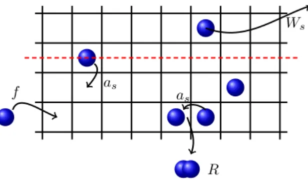
Formation of H2 on interstellar surfaces: Drawing on the example of hydrogen formation on interstellar dust grains, we investigate the influence of disorder on diffusion-mediated reactions on two-dimensional surfaces . As the most abundant element in space, H and H2are involved in an immense number of reactions and reaction networks that lead to the formation of complex molecules.

Nevertheless, the fundamental formation of H2 via H + H→H2has not been fully understood so far. Due to the low temperatures and pressures in space, this reaction is not efficient for two atoms meeting in three-dimensional space.

It has been agreed on that the surfaces of dust grains in the interstellar medium act as catalysts and H2 is formed on these surfaces. Inspired by former work, we investigate in this thesis the influence of disorder in the surface’s binding energies on the reaction rate of molecule formation. We identify a uniform mechanism facilitating a high reaction rate even in temperature regions where a system without disorder performs poorly. This part is based on the publications [89,90]

and contains further efforts on general discrete binding energy distributions and multiple-species systems.

More details on the connection between the applications and the framework of reaction-diffusion systems will be given after the detailed introduction to each of the systems at the beginning of the corresponding part of this thesis.

For our investigations the following methods are employed:

analytical treatment: The stationary reaction-diffusion equations for both applications are analyzed with emphasis on simplified effective equations that capture the essence of the system’s behavior,

numerical treatment: Additional to the (effective) analytic solutions we also employ direct numerical solutions of the full (stationary) system in both parts of this work,

kinetic Monte Carlo simulations: In the second part of this work we also use simulations that capture the microscopic processes in detail. These simulations serve as a reference for both the analytical models and the direct numerical solutions.

1

Part I

Robustness in deterministic

mutation-selection models

3

Chapter 1

Introduction

The branch of population genetics, which tries to describe biological evolution in terms of natural selection, nowadays referred to as Neo-Darwinism or ’modern synthesis’, was founded in the 1920’s by Fisher, Haldane and Wright (see [33,42,91] and references therein).

Studies revealed the high complexity of molecular processes like reproduction or gene expression. The question is still not answered, which of the conceivable interplays between the elementary processes on the molecular level like for example genetic drift, mutations, selection or recombination, are the most important ones for the evolution of a whole species.

Theoretical models for evolution can - due to the complexity of the processes - typically capture only a few aspects found in the experiments. An important class of models are the ones assuming mutation and selection mechanisms to be the most essential ones. Even if these mechanisms are not as essential as assumed, they play an important role and thus worth studying them in detail.

The elementary processes found in these models can probably be used as case studies for models concerned with other aspects of evolutionary processes. For reviews about this topic see [3] or [27].

Here, we will restrict ourselves to mutation-selection models for the artificial case of infinite population sizes, the quasispecies models. That means influences like drift (due to fluctuations caused by finite population size) are neglected, which in turn provides us with some powerful possibilities of solving the emerging equations for the population’s state. The two famous models concerned with the influence of mutation and selection on large populations are the Crow-Kimura model established 1965, [53,50], and the Eigen model, invented 1971, [30].

Models: The Crow-Kimura (CK) and the Eigen model present the principal ideas of how mutations and reproduction can interfere in asexual, haploid organisms and in the regime of very large (“infinite”) populations. One possibility is that mutations occur steadily due to permanent influence of the environment, captured by the Crow-Kimura model, the other is that mutations occur only during reproduction as copying errors, as decribed by the Eigen model. For that reason the Crow-Kimura model is also known as parallel model and the Eigen model as coupled model. The two models are deterministic models in the sense of neglecting fluctuations due to finite population size. Therefore, the obtained results are only asymptotically correct for real populations. Furthermore, the

4 Introduction

CK-model, being a continuous time model, can be derived from the discrete time Eigen model via straightforward continuum limit in time (to first order). Though invented for another purpose, it turned out, that the Eigen model is adequate to describe bacteria under strongly controlled environmental conditions. We will present this model together with the Crow-Kimura model in chapter 2. The Crow-Kimura model can be used to describe the evolution of virus populations, which is used in the development of drugs against viral diseases. For more details about the context of the Crow-Kimura model see e.g. [53,50].

Fitness landscapes: The crucial additional ingredient needed in both models is the fitness landscape. It assigns to each information sequence (e.g.

DNA or RNA sequence) the expected number of offspring an individual with this sequence produces. Thus it provides information on the selection. In principle, this fitness landscape has to be measured for real populations in fixed environments, but this is a highly complicated issue. Hence, different simple and more complex shapes of fitness landscapes have been proposed and investigated theoretically, starting with Eigens sharp-peak landscape [30], where only one sequence has a better fitness than all others. A theoretical analysis is, for example, concerned with the qualitative and quantitative shape of the equilibrium population distribution, occurring phase transitions between qualitative different distributions, scaling behavior for infinitely long sequences, etc. Some cases can be solved analytically, but for most of them, one has to rely on numerical methods. Examples of important landscapes are the mentioned sharp-peak landscape, the Fujiyama landscape, the plateau landscape, rugged fitness landscapes or epistatic landscapes. For a review about all mentioned landscapes see [51]. A discussion about how and to what extent these kinds of landscapes can be be inferred from experiments can be found in [85]. For several of these landscapes, experimental evidence exists [17,10,87,15].

In this thesis, we are concerned with the class of epistatic fitness landscapes, especially with the most extreme variant, the plateau-shaped landscape. In the latter, a high fitness value is assigned to all sequences that differ from the best-adapted one only by a defined maximal number of sites. All other sequences have a very low fitness. A central question we adress is under which conditions and to what extend a broader plateau is preferable to a higher fitness value, regarding the mean fitness of the whole population. To answer this question it is first necessary to understand the fitness effect of one plateau on a quasispecies population.

Connection to the framework of reaction-diffusion models: To apply the general reaction-diffusion equation (1) to a specific problem, the reaction term has to be specified. Like Fisher and Kolmogorov applied the specific form ofR(u) =u(1−u) in (1) to describe gene spreading in a population, in [29] Ebeling et al. consider the class of reaction termsR(u) =w(x, u)u(x, t) with arbitrary real functionw. Their main application is a generalization of Fisher’s classical population genetics model [33]. They show in detail that the generalized Fisher model can be regained from the reaction-diffusion equation (1) by their choice of the reaction term. Now, the Eigen model, whose continuous time version — the Crow-Kimura model — we study in this thesis, is the space-discretized version of Fisher’s model. In this sense, the evolution models investigated here, belong to the great class of phenomena that can be described by reaction-diffusion models. In particular, Ebeling et al. derive a Schr¨odinger type equation for the time behavior of their system’s solution (eq. (3.5) in [29]),

5

which is of exactly the same shape as equations (3.7) and (3.11) we provide in chapter3 for the mean fitness of the population.

Outline

In the first section of chapter2we start with the explanation of the basic biological concepts and continue in section 2.2 with the definition of the Eigen and the Crow-Kimura model. Having understood the basic principles, we introduce and exemplify the notion of fitness landscapes in section2.3and specify the term of the error threshold in section2.4. Equipped with this knowledge, we review a popular method of solving the dynamical equations of the Eigen model and the Crow-Kimura model for the equilibrium state, in the limit of infinite sequences, called maximum principle, in section2.5. The knowledge presented in the whole chapter2is well known in the field and provides the background for our analysis starting in chapter3with the calculation of the equilibrium state of a population in a plateau-shaped fitness landscape (also called mesa landscape) for finite sequence length. We calculate finite sequence length corrections to the maximum principle, thereby improving the accordance of analytical and numerical results significantly. For the calculations we exploit an analogy to quantum mechanics and map the systems equation of state to a Schr¨odinger equation. All results are confirmed by numerics in section 3.5. After this comprehensive analysis of fitness landscapes with one mesa, we turn in chapter 4to the competition between selection and robustness, also called survival of the flattest. The so far derived results are used to answer the question in which cases more robustness is preferable to higher selection values. We find that for finite sequence lengths, a broader but smaller fitness plateau can maintain a population at large mutation rates, where a higher but narrower plateau already fails. In the limit of infinite sequence length and fixed plateau widths, the higher plateau always provides the highest fitness for the population. We provide a formula for the critical sequence length, beyond which only the higher plateau can maintain a localized population. Additionally, the notion of the ancestral population is introduced and discussed for mesa-shaped fitness landscapes with two plateaus. Before drawing a final conclusion in chapter6we discuss the occurrence of the error threshold in a general epistatic landscape in chapter 5, thereby improving a previous result [86].

6

7

Chapter 2

Basic principles

In this chapter we introduce the basic concepts and notions of population genetics and dynamics needed. We focus on so-called deterministic mutation-selection- models for haploid asexual species, the quasispecies models. Haploid means that each individual of the species contains only one string of information (e.g.

the DNA or RNA string). Asexual means that each individual can produce offspring autonomously, e.g. via cell division, and deterministic refers to an infinite population size. So we are in a context that allows for description of large populations of bacteria and viruses, but not higher developed organisms.

Due to their simplicity, these quasispecies models can serve as toy models to find e.g. the characteristics of a certain fitness landscape.

2.1 Terms and definitions

As indicated in the introduction (chapter1), we can characterize the individuals of the considered species by the string they carry. This string σ= (s1, .., sL), of lengthLcontains letterssi∈ Awhich are taken from an alphabetAof size

|A| ≥2. In classical population genetics this string is just the DNA or RNA of an individual, so the alphabet A is of size four and there are 4^L possible sequences which form the sequence space¹. In the simplest case the two letters AandGand the lettersC andT (U) are pooled respectively asA andGare purins andCandT (U) are pyrimidines. These are to some extent exchangeable.

Then we get an alphabet consisting of 2 letters A={+1,−1} and 2^L possible sequences. If we connect all sequences of the set of all possible sequences in such a way, that a connection is made between all sequences that differ only by one site, we get the sequence space with the topology of a hypercube, an illustration of which can be seen in figure2.1.

As is known from evolutionary biology, individuals well-adapted to their environment have the best chance to produce a large number of offspring, thereby passing on their information sequence. The fraction of not well-adapted individuals is diminished over time, dies out or survives only by mutation effects, as the individuals produce less offspring. If we assume that an information

1Depending on the posed question also other information strings can be taken to characterize the individuals. For example it can be the information of the gene configuration of the individual (which allele of a certain gene this individual has).

8 Basic principles

1¯11¯1

¯1¯1¯11

¯11¯11

11¯11 1111

¯1111 1¯111

111¯1

¯1¯111

¯111¯1 1¯1¯11

11¯1¯1

¯1¯11¯1

¯11¯1¯1

1¯1¯1¯1

¯1¯1¯1¯1

Figure 2.1: Illustration of the sequence space for binary sequences of length four with an alphabet consisting of ±1. The letter −1 is abbreviated ¯1 in the picture. The sequence space has a hypercubic topology.

string σ = (s1, .., sL) characterizes the individuals, a quantifying degree of adaptation should be connected with each of the possible sequences. This degree of adaptation is usually called the fitness and its value is connected to the effective number of offspring an individual produces per unit time. In the context of population genetics the fitness is usually assigned to the genotype instead of the phenotype because the connection between the two is complicated and mostly unknown².

We assume the generations of the considered population to be non-overlapp- ing and the generation time to be normalized to one. Then we can describe the evolution of this species by a discrete time model where the time takes discrete values 1,2..., according to the actual generation. For a discrete time model the fitnessFσ then is the expected number of offspring an individual with sequenceσproduces. It is also called the Wrightian fitness. We can now perform a continuum limit in time, corresponding to the limit of small generation time

∆t→0, such that the total amount of offspring produced in a finite time span is constant. Then the number of offspring is reduced, when the individuals’ lives are shorter, and we also have to perform a continuum time limit in the fitness functionFσ. We write

Fσ≡e^wσ∆t (2.1)

and callwσ theMalthusian fitness. Sending the generation time ∆tto zero, we find to first order in time

Fσ≡e^wσ∆t≈1 +wσ∆t , for ∆t→0 . (2.2)

2All individuals with a certain sequenceσ^∗belong to the same genotype. The phenotype comprises all genotypes that produce the same characteristic traits of individuals. The mapping from geno- to phenotype is thus typically from many to one. A simple example is the formation of amino acids by triplets of the nucleotides. There are 20 amino acids but 4³= 64 possible combinations of three nucleotides (of which there are four different ones). So several combinations of nucleotides lead to the production of the same protein.

2.1 Terms and definitions 9

The Malthusian fitness is the important quantity for a continuous time model, like the Wrightian fitness is for the discrete time models. Equation (2.2) reflects the idea of reduced offspring for smaller generation times. As next step, we also want to include the effect of mutations either due to the environment or due to copying errors during reproduction. On the level of genes and nucleotides a mutation changes a sequence into another one, for example by changing single sites. This basic type of mutation is called point mutation. We concentrate in this work on point mutations only. If we assume that the mutation probability µis uniform throughout the whole sequence and is the same for all letters in the alphabet, we can write down the mutation probability for an abitrary sequence σto mutate into another arbitrary sequenceσ⁰ as

Qσσ⁰ = µ

|A| −1

k(σ,σ⁰)

(1−µ)^{L−k(σ,σ0)} . (2.3) The first factor accounts for the probability that the differing sites are mutated into each other, while the second factor represents the probability that the other, already matching sites do not mutate. Here

k(σ, σ⁰) = 1 2(L−

L

X

i=1

sis⁰_i) (2.4)

is theHamming distanceof the two sequencesσandσ⁰, which is just the number of different sites. The mutation probabilityQσσ⁰ is the same for all sequencesσ⁰ which have Hamming distancek to sequenceσ. The numberNk of sequences with the same Hamming distance to sequenceσis

Nk= L

k

(|A| −1)^k . (2.5) Qσσ⁰ is a real probability as P

σQσσ⁰ = 1. This normalization condition simply states that the sequenceσ⁰ mutates to some other sequence — or stays the same. When performing the continuous time limit we need to change from mutation probabilities to mutation ratesησσ⁰. This is done by

Qσσ⁰ ≈δσ,σ⁰ +ησσ⁰·∆t, for ∆t→0 . (2.6) If we denote the mutation rate per letter by ˜µand setµ= ˜µ∆t then

ησσ⁰ =







0 , k(σ, σ⁰)>1

˜

µ , k(σ, σ⁰) = 1

−µL˜ , k(σ, σ⁰) = 0

(2.7) The normalization condition reads P

σησσ⁰ = 0. A review about the topic of mutation and selection can e.g. be found in [3].

A special class of fitness landscapes are the so-calledpermutation-invariant fitness landscapes, in which only the number of mutations away from the wild type sequenceσoand not their position is important for a sequence’s fitness. In mathematical terms, this meanswσ=wk(σ,σo). Though being a simplification, permutation-invariant fitness landscapes are applicable to relevant systems, like to the binding energies of proteins to binding sites in the regulatory region of a gene [39].

10 Basic principles

2.2 Models

2.2.1 Eigen model

To describe the evolution of the population, we need to specify the interplay between the different ingredients. Here we take into account only mutations occurring as copying errors during reproduction and deterministic evolution³. For finite generation time this situation is described by the Eigen model [30].

In consequence, the fraction of individualsPσ(t) carrying sequenceσat timet evolves to the next generation according to

Pσ(t+ 1) = P

σ⁰Qσσ⁰Fσ⁰Pσ⁰(t) P

σ⁰Fσ⁰Pσ⁰(t) . (2.8) Σσ⁰ runs over all possible sequences and for binary sequencesQσσ⁰ is given by

Qσσ⁰ =µ^k(σ,σ0)(1−µ)^{L−k(σ,σ0)} . (2.9) Again k(σ, σ⁰) is the Hamming distance between the sequencesσandσ⁰. We notice the fact, that the model is invariant under multiplication of the fitness by a constant factorFσ→C·Fσ. The equations can be linearized by changing to an unnormalized population distributionZσ(t) via [51]

Zσ(t) =Pσ(t)

t−1

Y

τ=0

X

σ⁰

Fσ⁰Pσ⁰(τ), (2.10) at the cost of non-locality in time. We then arrive at the linear equations

Z(σ, t+ 1) =X

σ⁰

Qσσ⁰Fσ⁰Zσ⁰(t). (2.11) This linearized version is easier to solve, when calculating stationary states.

By renormalization of the resultZ^∗(σ), we regain the normalized population distribution P^∗(σ). But for convenience we will in the following work with a continuous time model, the Crow-Kimura model, which can be inferred from (2.8) by the limit generation time ∆t→0 as shown below.

2.2.2 Crow-Kimura model

To derive the proper continuous time evolution from the discrete time model (2.8), we use (2.2) and (2.6) to paraphrase the dynamics for short generation

time ∆t. WritingPσ(t+ ∆t)≈Pσ(t) + [dtPσ(t)]∆t, we find dtPσ(t) = (wσ−w)¯ Pσ(t) +X

σ⁰

ησσ⁰Pσ⁰(t). (2.12) Therein ¯wis defined through ¯w= Σσ⁰wσ⁰Pσ⁰(t). Now we assume the (Malthusian) fitness to be a function wk only of the Hamming distance k to the optimal sequence atk= 0. Then, surpressing the time dependence, renaming the point mutation rate ˜µ→µand using (2.7), we can rewrite (2.12) to the final and here needed formulation of the Crow-Kimura model

dtPk= (wk−w)P¯ k+µ(k+ 1)Pk+1+µ(L−k+ 1)P_k−1−µLPk, (2.13)

3achieved by assuming infinite population size

2.2 Models 11

with 1 ≤ k ≤ L−1. For k = 0 and k = L the equations obviously have to be modified. Still, the deterministic character of this equation is justified by an infinitely large population. The nonlinearity introduced by the mean (malthusian) fitness ¯w(t) = P

kwkPk can be eliminated by passing again to unnormalized population variables via the transformation [51,80]

Zσ(t) =Pσ(t)·exp



 X

σ⁰ t

Z

0

dτ Pσ⁰(τ)



. (2.14)

The resulting linearized CK-model for the case of fitness landscapes only de- pending on the Hamming distance then reads

dtZk(t) = (wk−µL)Zk(t) +µ(k+ 1)Zk+1(t) +µ(L−k+ 1)Z_k−1(t). (2.15) From the solution of this linearized set of equations, the normalized solution can be reconstructed via

Pk(t) = Zk(t) P

k⁰Zk⁰(t). (2.16)

In the following we will be concerned with the equilibrium states of (2.13), or rather (2.15). The stationary states can be found by the separation ansatz

Pk(t) = e^λtP_k^∗. (2.17)

implying the largest of all possible eigenvalues Λ = max λ to dominate the behavior of the system in the long-time limit. In the corresponding eigenvalue equation

ΛP_k^∗= (wk−µL)P_k^∗+µ(k+ 1)P_k+1^∗ +µ(L−k+ 1)P_k^∗₋₁

=:M_k,k0P_k^∗0 ∀k= 0, ..., L

⇔ΛP^∗=MP^∗

(2.18)

theL×Lfitness-mutation-matrixMonly consists of real non-negative entries.

So the Perron-Frobenius theorem is applicable here, ensuring the existence of an unique, positive, and real largest eigenvalue Λ, and a corresponding principal eigenvectorP^∗ that only has non-negative entries. This eigenvalue Λ is equal to the long-time limit of the mean population fitness ¯w, as can be seen by inserting the stationarity conditionPk(t) =P_k^∗ into (2.13) using (2.18), and it is the main quantity of interest in this work. The CK-model is invariant under additive shifts of the fitness,wk→wk+c, as counterpart to the Eigen model.

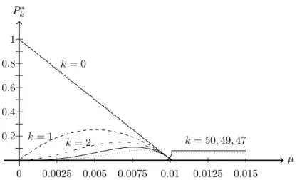
In figure 2.2 the equilibrium population P_k^∗ of the CK-model is shown as function of the mutation rate per letterµfor a single peak landscapewk =δk,0

and a sequence length ofL= 100. With growing mutation rate, the population becomes uniformly distributed in sequence space, a phenomenon called error threshold, which will be discussed in the next section.

We will work with the Crow-Kimura model for the rest of this first part, as the continuous time formulation is more convenient to handle and the derived results are qualitatively also valid for the Eigen model.

12 Basic principles

µ P_k^∗

0 0.0025 0.005 0.0075 0.01 0.0125 0.015 0.2

0.4 0.6 0.8 1

k= 0

k= 1

k= 2 k= 50,49,47

Figure 2.2: Part of the equilibrium population distribution of the quasispecies popu- lation in a sharp-peak landscapew(k) =δk,0 with sequence lengthL= 100. Shown are the normalized population fractionsP_k^∗for different Hamming distancesk. Some very important ones are labeled in the picture. The data is obtained numerically, as described in section3.5.

2.3 Fitness landscapes and robustness

The still missing ingredient of our population model is the fitness landscape.

These landscapes typically serve as toy functions, in the hope, that the model captures some important aspects of reality. In the last section, we already introduced one important class of fitness functions, the permutation invariant landscapes. To this class — to which we will stick in this work — belong several famous landscapes, like thesharp-peak landscape, introduced by Eigen [30]

wk =w0δk,0, w0>0, (2.19) where only the master sequence has a high fitness. This reflects an extreme kind of epistasis (see below). It is applicable, if e.g. the environment sets very strong conditions on the population. In theFujiyama (or multiplicative) landscape

wk=w0−b·k , w0, b >0 (2.20) every mutation away from the master sequence reduces the fitness by the same amount, while inepistatic landscapes like [86]

wk =w0−b·k^α , w0, b, α >0 (2.21) the reduction depends on the number of already occured mutations. Depending on the epistatic factorαevery additional mutation away from the master sequence is punished more (α >1) or less (α <1) than the previous one. We will discuss the case of epistatic landscapes in detail in chapter5. In these two latter types of landscapes, mutations are non-lethal (in the way which will be discussed in sec. 2.4 below) but lead to a reduction of offspring. In the corresponding populations we typically find mutational variety and the width of the population

2.4 Error threshold 13

k

wk Pk

k0 L/2 L

0.2 0.4 0.6

0.8 0.16

0.12 0.08

blah

P_k,deloc^∗ P_k,loc^∗

Figure 2.3: Equilibrium population distribution for the localizedPk,loc and delocalized P_k,deloc^∗ population distribution, as function of the Hamming distancekin a plateau- shaped fitness landscape with a plateau widthk0. The lefty-axis belongs to the fitness (dashed line), the righty-axis to the population distributionsP_k^∗. We see the localized population to reside mainly at the edge of the plateau as due to the mapping from sequence to Hamming space, the number of sequences there is larger than atk= 0.

The delocalized population is normally distributed around the Hamming distanceL/2.

distribution (in Hamming space) depends on the mutation rate, as well as on the parameters of the landscape.

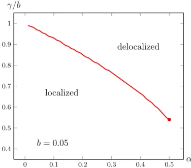
Coming back to our concerns, we want to discuss the effects of robustness on a population. This is a concept of central importance in current evolutionary theory [26,55]. Here we address specificallymutational robustness, which we take to imply the stability of some biological function with respect to mutations away from the optimal genotype. To be precise, suppose the genotype is encoded by a sequence of lengthL, and the number of mismatches with respect to the optimal genotype is denoted byk. Robustness is then quantified by the maximum number of mismatchesk0, that can be tolerated before the fitness of the individual drops significantly below that of the optimal genotype atk= 0. This situation arises e.g. in the evolution of regularity motifs, where the fitness is a function of the binding affinity to the regulatory protein [39, 9]. Thismesa-shaped fitness function is the simplification of a Fermi function at low temperatures, which in turn appears e.g. in simple thermodynamic models for the binding probability of a transcription factor to a regulatory region. Assuming that the fitness is independent of k both for k ≤ k0 and for k > k0, the fitness landscape is parametrized by the widthk0 and heightw0 of the mesa [68]. In figure2.3, a (permutation invariant) mesa-shaped fitness landscape and the corresponding localized and delocalized population distribution in Hamming space are depicted.

In the following we will especially analyze this type of mesa landscapes and come later on to the more general case of epistatic landscapes. We use the terms mesa and plateau landscape interchangeably.

2.4 Error threshold

Depending on the shape of the fitness function and the mutation rate per letter µ, in quasispecies models a localization-delocalization phase transition, also callederror threshold can occur. At this threshold the population undergoes a transition from a localized state around the fittest sequence(s) to a population homogeneously spread in sequence space (which corresponds to a binomial distri-

14 Basic principles

bution in Hamming space). For a population this transition can be interpreted as insensitivity towards changes in fitness or as the extinction of the (real) finite population to which the model is applied to.

To analyze any transition in which the mean Hamming distance of a popula- tion changes⁴, the population averaged “magnetization”M, defined by

M = 1−2hxi ∈[−1,1] with hxi= 1 L

L

X

k=0

kP_k^∗, (2.22) is a convenient though not fundamental quantity — the principal eigenvalue Λ of (2.18) is the fundamental quantity determiningP_k^∗. If the whole population only consists of master sequences (k = 0 by definition), the magnetization is M = 1. If only the inverse master sequence is present, the magnetization becomesM =−1. For a uniform distribution in sequence space (delocalized population) the magnetization isM = 0. Thus we can in most cases distinguish the qualitatively different states a population assumes under different mutation rates (except the mentioned pathologic cases), by considering the population averaged magnetizationM as a function ofµ. There are some special cases, where only the observation of the magnetization becoming zero is not sufficient, like in the case of the Fujiyama (or multiplicative) landscape, where the population remains localized but its average Hamming distance is — with growing mutation rate — continuously shifted towardsk=L/2 . Then we have to retreat to the analysis of the quality of change of either the population mean fitness Λ(µ) or the magnetization.

To obtain meaningful results in the limitL→ ∞, the mutation probability has to be scaled to zero accordingly,µ→0,⁵. Another possible scaling — we do not adopt here — is to scale the fitness∝L. For most fitness landscapes a scaling withµL= const.is appropriate, but the right scaling can often only be obtained from the calculation of the critical mutation rate (error threshold)µtr

itself. An example for a landscape where the scalingµL= const is inappropriate is the epistatic landscape which will be discussed in chapter5.

The order of the phase transition is somewhat delicate to estimate. The intricacy lies in the sequence of performing limits. As we here will frequently use numerics to confirm our analyical results, we always work with finite sequence lengths. So, the limit of infinite sequence length is the last one to be performed.

For finite sequences we see the error threshold to resemble a second order phase transition. For this reason, we will here consider the error threshold to be of second order. When estimating the order of the transition after performing the infinite sequence length limit, the error threshold will be of first order, as the order parameter performs a discontinuous jump fromM = 1 atµ= 0 toM = 0 atµ6= 0. Though we have to point out here, that the error threshold, in the sense of a proper physical phase transition only exists in the limitL→ ∞. This discussion is also taken up in the paper by Tarazona [79] in the context of a treatment of the models as Ising chains. Nevertheless, other opinions on the order of the error threshold and which order parameter should be taken exist.

For a different view on the topic see e.g. [44].

4pathologic cases like a (changing) population distribution symmetric tox= 1/2 are not covered!

5otherwise the mutation probability per sequence would diverge

2.5 The maximum principle 15

2.5 The maximum principle

So far, we have presented the basic ingredients and how they enter into the models.

Now we turn to finding the equilibrium state and the growth rate of a population in a given environment (represented by the fitness function). Therefore we have to solve the set of equations (2.18). To its solution, a considerable body of work has already been devoted for largeL. If, in addition to the scaling constraints onµ, the fitness landscapewk is assumed to depend only on therelative number of mismatches, such that

wk →f(x), x=k/L, (2.23)

then forL→ ∞, the principal eigenvalue in (2.18) is given by the solution of a one-dimensional variational problem as [44, 2,74,67,73,4]

Λ = max

x∈[0,1]{f(x)−γ[1−2p

x(1−x)]}, (2.24) whereγ=µL. Moreover, iff(x) is differentiable the leading order correction to (2.24) takes the form [67,73]

∆Λ = γ

2Lp

xc−x²_c[1−q

1−2f⁰⁰(x^∗)(xc−x²_c)^3/2/γ], (2.25) where xc is the value at which the maximum in (2.24) is attained. Therefore, we need other methods when analyzing the main features of robustness using a mesa-shaped fitness landscape of the form

wk=

w0>0 : 0≤k≤k0

0 : k > k0, , (2.26)

aswk is not differentiable any more. Herew0 denotes the selective advantage of the functional phenotype andk0 is the number of tolerable mismatches. For scaling landscapes (2.23), here realized by

f(x) =w0Θ(x−x0), (2.27)

where Θ(x) is the Heaviside function and x0 = k0/L, at least the maximum principle can be applied (x0<1/2) to yield

Λ =

w0−γ(1−2p

x0(1−x0)) , w0> w^c₀

0 , w0< w^c₀ (2.28)

withw^c₀=γ(1−2p

x0(1−x0)). The value w₀^c of the selective advantage marks the location of the error threshold at which the population delocalizes from the fitness plateau and the locationxcof the maximum in (2.24) jumps fromxc=x0

toxc= 1/2.

To calculate the leading order correction ∆Λ to the maximum principle for finite sequence length in the next chapter, we will clarify and use an analogy to quantum mechanics, thereby rederiving the maximum principle (2.24), and we will show that ∆Λ is of orderL^−2/3 orL^−1/2 rather thanL⁻¹in the case of the pure maximum principle for scaling landscapes.

16

17

Chapter 3

Continuum limit in Hamming space

We want to solve the problem of finding the influences and limits of robustness in deterministic mutation-selection models. Robustness is implemented as a plateau-shaped fitness function into the Crow-Kimura model as introduced above. Based on the existing approaches, we clarify the connections between these different accesses and use a formal analogy to quantum mechanics to finally solve the issue of mutational robustness. Therefore, we first derive a description of the CK-model in a continuous Hamming space. Then we are able to find a finite size correction in harmonic approximation and beyond, using an analogy to quantum mechanics. Here we can connect to the work of Gerland and Hwa [39]. As reference method, we study the system by means of direct numerical calculations and find the analytical results verified.

3.1 Analytical derivation in harmonic approxi- mation

A natural ansatz to analyzing (2.18) for large sequence lengthsLis a continuum limit in Hamming space, that is in the index k. Therefore, we introduce the small parameter= 1/Land replace the population variablePk by a function

φ(x) = lim

L→∞PxL. (3.1)

Furthermore we assume the fitness to be of the general form (2.23). By expanding the finite differences in (2.18) up to second order in, we get a differential equation of second order,

f φ−γ d

dx[(1−2x)φ] + ²γ 2

d²

dx²φ= Λφ, (3.2)

which is a stationary drift-diffusion equation. By changing back to the unscaled variablek=Lx, we can see, that the equation is identical to the one obtained by Gerland and Hwa [39]. Nevertheless, we will see thatxis the proper variable to perform the continuum limit, not the least because it fulfills the mathematical constraint of a compact support.

18 Continuum limit in Hamming space

In order to solve equation (3.2) it is advantageous to eliminate the first-order drift term, which can be done by the transformation

φ(x) =p

φ0(x)ψ(x), (3.3)

with

φ0(x)∝exp[−(1−2x)²/(2)]. (3.4) It is easy to see, why this transformation symmetrizes the linear operator in (3.2). In the absense of selection,f = 0, the principal eigenvalue in (3.2) is Λ = 0, and the corresponding (right) eigenvalue is a Gaussian centered atx= 1/2 and thus just given by (3.4). This Gaussian is the central limit approximation of the binomial distribution

P_k⁰= 2^−L L

k

, (3.5)

which solves (2.13) forwk= 0 (∀k) and Λ = 0. It is well known that the central limit approximation of (3.5) is valid in a region of size√

Laroundk=L/2, but becomes imprecise for deviations of orderL.

The theory of large deviations provides an improved approximation by the ansatz

Pk∝exp(−Lu(x)) (3.6)

withu(x) being the large deviations function. This ansatz, which has been recently suggested for this problem by Saakian [74], will be explained in more detail in Appendix A.1.

And though we have just shown that the drift-diffusion approximation is only accurate nearx= 1/2, the center of the Hamming space, we will stick to this approach, as it allows a fundamental understanding of the problem. First, we can make contact with the work of Gerland and Hwa and second can we reformulate the eigenvalue problem in the language of standard quantum mechanics. The well developed formalism of quantum mechanics then allows to extend the solution of the eigenvalue problem beyond the second order approximation made in equation (3.2).

But coming back to solving the drift-diffusion equation (3.2), inserting (3.3) leads to the equation

−²γ 2

d²

dx²ψ+V(x)ψ=−(Λ−γ)ψ, (3.7) with

V(x) = γ

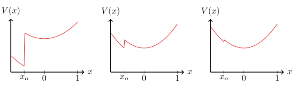
2(1−2x)²−f(x). (3.8) A sketch of V(x) for different values ofγand a mesa-shaped fitness landscape (2.27) can be found in Fig3.1.

Using standard quantum mechanics, we can interpret (3.7) as the stationary Schr¨odinger equation for a particle of mass 1/γexposed to the effective potential (3.8) and energy eigenvalue−(Λ−γ) in one dimension and space representation.

The potential is the superposition of a harmonic oscillator centered atx= 1/2 and the negative fitness landscape. The qualitatively different cases are depicted in figure3.1. As pointed out in [68], the inverse sequence lengthplays the role of Planck’s constant~, which implies that the case of interest is thesemiclassical

3.2 Extension of the harmonic approximation 19

x V(x)

xo 0 1 x

V(x)

xo 0 1 x

V(x)

xo 0 1

Figure 3.1: Sketch of the effective potential V(x) (3.8) for different values of the mutation rate γ. For small mutation rates (figure on the left), the population is localized on the plateau. At the critical mutation rateγc (figure in the middle) the ground state is degenerate and thus allows for a transition of the population from a localized (minimum atx=x0) to a delocalized (minimum atx= 0) state and vice versa. And for large mutation rates (figure on the right) the population is delocalized.

limit of the quantum mechanical problem. In particular, for→0 the ground state energy−Λ becomes equal to the minimum of the effective potential. We thus arrive at the variational principle

Λ = max

x∈[0,1][f(x)−γ

2(1−2x)²], (3.9)

which is precisely the harmonic approximation of the (exact) relation (2.24).

In the perspective of quantum mechanics, the error threshold corresponds to a shift between different local minima ofV(x), which become degenerate at the transition point. The transition is generally of first order, in the sense that the locationxc of the global minimum jumps discontinuously. Within the harmonic approximation the transition occurs at

w₀^c= γ

2(1−2x0)²≈ γ 2

1−4k0

L

(3.10) forx0=k0/L1, following the argumentation of section 2.5.

3.2 Extension of the harmonic approximation

The so-far used harmonic approximation aroundx= 1/2 breaks down near the boundariesx= 0 and x= 1. However, to access the regime 1k0 L, an accurate treatment of the region of smallx1 is clearly necessary, especially, since we want to connect to the work of Gerland and Hwa [39] who obtain a seemingly contradictory result for the critical plateau needed for a localized population. The quantum mechanical treatment can be extended such that it becomes quantitatively valid over the whole interval 0≤x≤1. Based on the considerations of [73], we then arrive at the modified Schr¨odinger equation (see appendixA.1for a derivation)

−²γp

x(1−x) d² dx²ψ+h

γ(1−2p

x(1−x))−f(x)i

ψ=−Λψ, (3.11) which differs from (3.7) in two respects. First, the potential (3.8) is replaced by

Vfull(x) =γ(1−2p

x(1−x))−f(x). (3.12)

20 Continuum limit in Hamming space

In the asymptotic limit→0 the principal eigenvalue is given by minimizing Vfull, which exactly recovers the maximum principle (2.24). Second, the mass of the quantum particle described by (3.11) becomes position dependent,

m(x)=b 2γp

x(1−x)−1

, (3.13)

which replaces the simple identificationm= 1/γb in the harmonic case.

3.3 Finite sequence length corrections

From the considerations of sections3.1 and3.2, we can infer correction terms to (2.24) for finite sequence lengths. Within the harmonic approximation, for finite but large sequence lengths = 1/L 1 we have to include quantum corrections to the classical limit solution (3.9). Assuming a smooth fitness functionf(x), the ground state wave function is localized near the minimum xc of the effective potential, and the shift in the ground state energy can be computed by a harmonic approximation ofV(x),

V(x)≈V(xc) +1

2V⁰⁰(xc)(x−xc)²=V(xc) +1

2[4γ−f⁰⁰(xc)](x−xc)². (3.14) Identifying 1/γ with the massm of the quantum particle and comparing the correction term to the potential of a harmonic oscillatorVhar=mω²x²/2, we find the frequency of the oscillator to be

ω= 2γp

1−f⁰⁰(xc)/4γ. (3.15)

By further exploiting this analogy, we find the ground state energy contribution of the correction term to be

E0=~ω 2 ∼= ω

2 =γp

1−f⁰⁰(xc)/4γ. (3.16) Re-inserting the results into (3.7), we get an expression for the leading order correction to Λ:

−²γ 2

d²

dx²ψ+V(xc)ψ

= −(Λ−γ+1

2ω)ψ (3.17)

=: −(Λ + ∆Λ)ψ. (3.18)

The correction term

∆Λ = γ L[1−p

1−f⁰⁰(xc)/4γ] (3.19) coincides with (2.25) evaluated forxc ≈1/2. Analogously, the width ξof the wave function can be estimated viaξ=p

~/(2mω) to be¹ ξ=p

γ/2ω=

√γ [8p

1−f⁰⁰(xc)/4γ]^1/4. (3.20)

1Note that, because of the factor√

φ0in (3.3), this is not equal to the width of the stationary population distribution.

3.3 Finite sequence length corrections 21

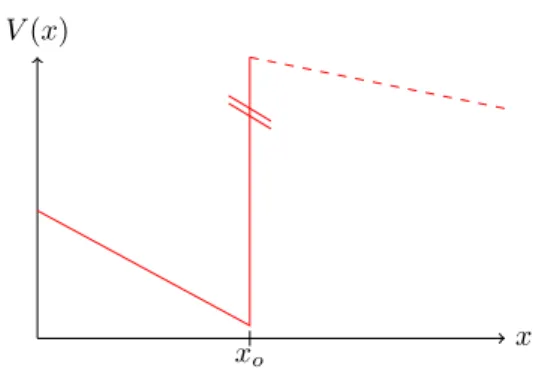
x V(x)

xo

Figure 3.2: Sketch of the effective potentialV(x) nearxc=x0. The slope left of the step is to first order given by−a=V⁰(x0). The height of the step isw0, which can

— for small— be considered as effectively infinite, since the kinetic energy of the particle is linear in.

In the case of the mesa landscape (2.27), the potential nearxc=x0consists of a linear ramp of slope

−a=V⁰(x0) = 2γ(2x0−1)<0 (3.21) followed by a jump of heightw0, see figure 3.2. For small, the jump can be considered as effectively infinite (as the kinetic energy of the particle is then very small since being linear in ) and we retrieve the well-known 1d-quantum mechanical ground state problem of a particle in a negatively sloped potential terminated by an infinitely high wall. The solution, provided by the Airy function, is standard textbook material, e.g. [71] and we obtain for our problem the prediction

∆Λ =z1(~²/2m)^1/3a^2/3= 2^1/3z1γ(1−2x0)^2/3L^−2/3+O(L⁻¹), (3.22) where z1 ≈ −2.33811... is the first zero of the Airy function. The scaling

∆Λ∼L^−2/3 was already noted in [68]. Again, the width of the wave function can be estimated and is of the order

ξ∼(~²/ma)^1/3∼^2/3 (3.23)

in this case. These considerations can also be applied to the extended solution of equation (3.11) in section3.2. Inserting (3.12) and (3.13) into the expression (3.22) for the finite size correction yields

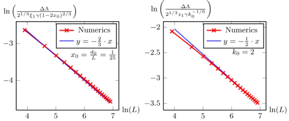
∆Λ = 2^−1/3z1^−2/3γ(1−2x0)^2/3[x0(1−x0)]^−1/6. (3.24) For fixedx0 this still scales as ^2/3=L^−2/3, but when takingL→ ∞at fixed k0, such that x0→0, we find instead that

∆Λ→2^−1/3z1γx⁻₀^1/62/3= 2^−1/3z1γk⁻₀^1/6L^−1/2. (3.25)

22 Continuum limit in Hamming space

3.4 Connection to former results

3.4.1 Review

A recent study on mesa-shaped fitness landscapes with finite sequence length was done by Gerland and Hwa (GH) [39]. They approach the problem by assuming from the outset 1k0L. So the maximal number of non-lethal mismatches is small compared to the sequence length. Then they perform the limit of infinitely long sequencesL→ ∞and focus on the regionkLat the same time, while keeping the Hamming distancekas the variable in which the limit is performed.

As an intermediate result they recover eq. (3.2) (in terms ofk), but then neglect the contribution 2k/L(corresponding to 2x) in the drift term. As a result the drift term becomes constant for allk.

In the localized regime, the stationary population distribution is of the form

φ(k) = e^kψ(k) (3.26)

in terms of the Hamming distance k. But the potential of the corresponding Schr¨odinger equation to (3.7) is given by −γ/2·f(x). Due to the ’zoomed in’

view on the system, the error threshold manifests itself in the non-normalizability of the solution or in other words, when ψ(x) decays as e^−x/ =e^−k. This is also the point, where the assumption of sufficient slow variation ofψ(k) on the scale ofk (needed for the continuum limit) is violated. Then for a broad fitness plateauk01, GH find a critical plateau height of

w^c₀=γ 2

1 +π²

k²₀

. (3.27)

This result clearly shows a dependence on the absolute number of allowed mismatches k0, but is independent of the sequence length L, apparently in contrast to (3.10).

3.4.2 Comparison

To understand the role and applicability of our results and the one of GH,we have to take a closer look on the validity of both approaches. For didactical reasons we start on the level of the harmonic approximation (sec.3.1) and then extend the comparison to the improved solution (sec.3.2). The harmonic approximation solution (3.10) is valid for largek0and breaks down, when the width of the wave functionξ becomes comparable to the potential well provided by the effective potentialV(x). In the case of the mesa landscape, this is tantamount to

ξ∼x0, (3.28)

which leads to

k0∼^−1/3=L^1/3 (3.29)

using (3.23) and x0 =k0. If we consider short plateaus withk0L^1/3, the ground state energy of the corresponding wave function can be estimated to

E0∼ ~²

md² ∼²γ x²₀ ∼ γ

k²₀, (3.30)