Spectroscopy from Fluid Surfaces
- Theory and Experiment -
Tuana Ghaderi
A thesis submitted in fulfillment of the requirements for the degree of Doctor of Natural Sciences in the subject of
Physics
Universit¨ at Dortmund
March 2006
I hereby declare that this submission is my own work and that, to the best of my knowledge and belief, it contains no material previously published or written by another person nor material which to a substantial extent has been accepted for the award of any other degree or diploma of the University, except where due acknowledgement has been made in the text.
Tuana Ghaderi March 16, 2006
I
Thesis advisors Author
Sunil K. Sinha Tuana Ghaderi
Metin Tolan
X-ray Intensity Correlation Spectroscopy from Fluid Surfaces
X-ray intensity correlation spectroscopy (XICS) is a coherent X-ray scattering technique, which enables the investigation of dynamic properties of matter by analyzing the temporal correlations among intensities scattered by the studied material. This novel technique has been intensively applied in the last decade in order to examine the temporal and lateral correlation properties of fluid surfaces.
Although, intensity correlation experiments are qualitatively well under- stood, present theoretical interpretations fail to explain XICS data from some well known fluid surfaces, such as water and glycerol. We believe that the discrepancies, between the theoretical predictions for the intensity correlation function and the experimental results, are due to some idealized assumptions with regard to the coherence of the X-ray beam, as well as the instrumental resolution.
This thesis is mainly concerned with the derivation of the intensity cor- relation function for surface sensitive X-ray intensity correlation experiments including the effects of partial coherence and instrumental resolution. In order to derive the intensity correlation function the theoretical approach is based in this work on the statistical properties of the fluid surface and the scattered electric field. A scalar wave equation for the electric X-ray field is derived to determine the field expressions from time fluctuating and inhomogeneous me- dia. The therefrom obtained field formulas are used to derive systematically field correlation functions and intensity correlation functions. The accuracy of the field expressions and the deduced correlation functions are restricted to the first Born approximation. Within this accuracy, we have provided inten- sity correlation functions that are applicable to charge scattering from fluid surfaces under the conditions of arbitrary spatial coherence and instrumental resolution. In addition, far and near field scattering conditions, i.e. Fraunhofer and Fresnel conditions, are rigorously incorporated in the theoretical intensity correlation functions.
The experimental part in thesis is dedicated to the analysis of XICS mea- surements from hexane and water surfaces. The data analysis is based in parts on the intensity correlation function which is derived in the theoretical part
II
iments. In contrast to the conventionally used intensity correlation formula, we have obtained very good agreement between our theoretical intensity cor- relation function and the experimental results from hexane. This work may therefore be of general interest to scientists who make use of XICS or other scattering techniques using partially coherent X-ray beams.
I would like to thank all the people who encouraged and supported me during the undertaking of this research.
Firstly, I would like to thank my supervisors, Prof. Dr. Sunil K. Sinha and Prof. Dr. Metin Tolan. Their support, encouragement, guidance and expertise has proved invaluable.
I would like to thank Dr. Christian Gutt, Dr. Michael Sprung and Zhang Jiang for many useful discussions regarding X-ray scattering and physics in general. I thankfully acknowledge their valuable assistance in setting up the X-ray scattering experiments at the European Synchrotron Radiation Facility in France and at the Advanced Photon Source in the USA.
I would like to thank my family and friends. Their support, encouragement and friendship will always be treasured. My greatest debt and heartfelt thanks goes to my wonderful parents, Arian and Shirin. They have been an inspira- tion throughout my life.
I save the last special thanks for T¨ulin, she has stood by me through the most difficult times of this process, offering her unconditional love and support. You are an inspiration, thank you.
V
Declaration I
Abstract II
Acknowledgments V
1 Introduction 1
2 Structure of Liquid-Vapor Interfaces 5
2.1 Hamiltonian Formalism for Liquid-Vapor Interfaces . . . 6
2.1.1 Capillary Wave Model . . . 6
2.1.2 Effective Interface Hamiltonian . . . 12
2.2 Surface Height Correlation Function . . . 16
2.2.1 Static Height Correlation Function . . . 16
2.2.2 Dynamic Height Correlation Function . . . 19
3 Elastic X-Ray Scattering From Rough Surfaces 23 3.1 Basic Principles . . . 24
3.2 Surface Scattering in First Born Approximation . . . 29
3.3 Distorted Wave Born Approximation . . . 44
3.4 Fresnel Effects . . . 48
4 Effects of Partial Coherence 53 4.1 Temporal and Spatial Coherence . . . 54
4.2 Diffraction of Partially Coherent X-rays from a Plane Aperture . 55 4.2.1 The van Cittert-Zernike Propagation Law . . . 55
4.2.2 Gaussian Schell-Model Source . . . 57
4.2.3 The Diffraction Solution . . . 61
4.3 Scattering of Partially Coherent X-rays from Arbitrary Media . 71 4.3.1 Generalized van Cittert-Zernike Propagation Law . . . . 72
4.3.2 Propagation of Field Correlations from a Scatterer . . . 74
4.3.3 Surface Scattering with Partially Coherent X-rays . . . . 80 VII
5 X-ray Intensity Correlation Spectroscopy from Fluid Surfaces 93
5.1 Scattering from Non-Static Media . . . 96
5.1.1 The Scattered Field in the First Born Approximation . . 99
5.2 Intensity Correlation Function Based on Siegert’s Relation . . . 101
5.2.1 Propagation of Scattered Field Correlations From Fluc- tuating Media . . . 102
5.2.2 Surface Sensitive XICS in first Born Approximation . . . 105
5.2.3 The General Resolution Function . . . 109
5.2.4 The Field Correlation Function for Gaussian Fluctuating Surfaces . . . 113
5.2.5 Examples . . . 118
5.3 Pusey’s Formulation of the Intensity Correlation Function . . . 132
6 Experimental Part 137 6.1 ID10A Beamline Description . . . 137
6.2 Measurement and Analysis of XICS data from Hexane . . . 138
6.2.1 Experimental Setup . . . 140
6.2.2 Results and Discussion . . . 142
6.3 Measurement and Analysis of XICS data from Water . . . 148
6.3.1 Experimental Setup . . . 148
6.3.2 Results and Discussion . . . 149
7 Conclusions and Future Research 153 7.1 Conclusions . . . 153
7.2 Future Research . . . 154
A Gaussian Statistics 157 A.1 Definitions . . . 157
A.2 Bloch Theorem . . . 159
A.3 Classical Baker-Hausdorff Theorem . . . 159
A.4 Siegert’s Relation for (real) random variables . . . 161
A.5 Applications to Surface Fluctuations . . . 162 B Alternative Calculation of the Intensity Correlation Function163
References 168
Introduction
X-ray scattering has a long history of significant contributions to widely vary- ing fields of scientific study. The scientific progress and outcome from X-ray scattering experiments has always been closely related to the availability and improvements of high brilliance synchrotron sources. Since the insertion of undulators and wigglers in synchrotron facilities so-called 3rd generation syn- chrotron sources are available, which produce a partially coherent X-ray beam.
This significant improvement of synchrotron sources has substantially enriched conventional X-ray scattering experiments by many new types of coherent X- ray scattering techniques. For instance, a number of laser light experiments, such as holography, intensity correlation spectroscopy, phase contrast imaging etc., can nowadays be implemented with partially coherent X-rays for opti- cally opaque materials and, in principle, with even higher spatial resolution.
Due to these promising advantages much effort has been put into the design of scattering experiments using coherent X-rays in the last few years [65].
This thesis concerns exploiting the partial coherence of synchrotron radi- ation in order to carry out X-ray intensity correlation spectroscopy (XICS) experiments from fluid surfaces. Such experiments, which are also known as X-ray photon correlation spectroscopy (XPCS), promise exciting new insights into dynamical phenomena in condensed matter, occurring on shorter length scales than can be reached in dynamical light scattering (DLS). Specifically, the partially coherent illumination of a random surface height distribution yields a random interference pattern, which is referred to as a speckle pattern. This speckle pattern changes in time, if the surface height distribution undergoes different states in time. The intensity correlation spectroscopy method reveals the characteristic times of the sample via time correlation of the scattered intensity in the speckle pattern. The basic ideas of XICS experiments from dynamic surfaces are schematically illustrated in Fig. 1.1. It is conventionally assumed that the time dependent part of the resultant intensity correlation
signal G2(τ) is essentially related to the surface height correlation function Cezz(τ) of the sample via
G2(τ)∝ |Cezz(τ)|2, (1.1) whereτ represents the correlation time. The measurement of the intensity cor- relation signal at different wave vector transfers eventually yields the dynamic properties of the surface at different length scales. The intensity correlation signal is, in a broader sense, also related to the intermediate scattering function [96, 66]. (A detailed discussion is given in chapter 5.)
Although, the above concepts appear plausible for surface sensitive XICS experiments, some experiments from relatively well understood fluid surfaces could not be interpreted by formulas that are essentially of the same form as eq. (1.1) [36, 85]. The most obvious discrepancy between eq. (1.1) and the experimental results in Ref.[36, 85] is the observation of a heterodyne intensity correlation signal, which refers to a linear relation betweenG2(τ) andCezz(τ).
This thesis shows that the consideration of partial coherence and finite in- strumental resolution are of central importance for the interpretation of XICS experiments from fluid surfaces. It is demonstrated that the influences of par- tial coherence and finite instrumental resolution can, for instance, lead to the observation of heterodyne intensity correlation signals. In the experimental part of this work we present XICS experiments on hexane and water surfaces.
The interpretation of the intensity correlation signal from both liquids depend vitally on the consideration of coherence and resolution effects. In order to account for these effects we have derived a formula for the intensity correla- tion function, which allows, in contrast to conventional formulas, a reasonable interpretation of our XICS experiments.
The structure of the thesis and a short description of the content in each chapter is given below.
Chapter 2summarizes the statistical properties of fluctuating fluid surfaces.
Some central predictions from the capillary wave model and the density func- tional theory for fluid surfaces are in detail discussed. Static and dynamic surface height correlation functions are derived for low and high viscosity flu- ids. The provided surface height correlation functions are continuously used throughout this thesis to interpret the surface scattering experiments.
Chapter 3presents the established description of elastic X-ray scattering from rough surfaces. Some approximation methods for constructing the specularly scattered X-ray intensity and the diffusely scattered counterpart are discussed in detail. A number of relations between the scattered X-ray intensity and the
Figure 1.1: Schematic illustration of XICS experiments from dynamic sur- faces. A coherent or at least partially coherent X-ray beam is scattered from a temporally fluctuating surface. The scattered intensity distribution yields a speckle-like interference pattern, which equally changes in time. The detec- tion and time correlation of the scattered intensity reveals dynamic properties of the sample surface under study. The probed length scale from the sample surface depends on the detection position of the intensity correlation signal.
static surface height correlation function are provided. Furthermore, we have eliminated an unphysical singularity in the conventional intensity formulas for surface scattering. The conditions for Fraunhofer and Fresnel scattering situ- ations are finally explored.
Chapter 4is concerned with conditions of partial coherence in X-ray scatter- ing experiments from static media. The propagation, diffraction and scattering of partial coherent X-rays are discussed in terms of mutual coherence functions.
The diffraction of partially coherent X-rays from a square slit is explained in detail. This demonstration example is used as a guidance to develop scatter- ing formulas from more complicated systems. The mutual coherence function for surface scattering conditions is constructed and examined for a variety of experimental situations. Surface sensitive scattering conditions are discussed in particular.
Chapter 5 presents a theoretical description of surface sensitive XICS ex- periments from fluid surfaces. The proposed intensity correlation function is based on statistical properties of the fluid surface, as well as the scattered fields. The conditions of partial coherence, instrumental resolution, and Fresnel scattering are accounted for in the discussion. The predictions of this intensity correlation function are finally compared with the conventionally used formula.
Chapter 6 presents surface sensitive XICS measurements from hexane and water. The data analysis was performed with the conventionally used intensity correlation function, as well as with the formula which is proposed in chapter 5.
By using the latter formula for hexane, we have obtained reasonable results for the surface tension and the kinetic viscosity. In contrast to these results, the data analysis with the commonly used intensity correlation function yielded values for kinetic viscosities which are several times larger for both liquids.
Chapter 7 summarizes the main findings of this thesis. A discussion on future research based on this work is given as conclusion.
Structure of Liquid-Vapor Interfaces
The challenging problem in equilibrium theories of liquid-vapor interfaces is to explain the density profile in the interfacial region, and to incorporate the role of surface tension, as well as the viscosity from a molecular point of view.
The first approach to this problem was developed for ideal liquids (viscosity free) by Van der Waals, almost one century ago. The mean-field, or Van der Waals theory of interfaces, introduces a laterally flat intrinsic density profile that changes gradually from the mass density of the liquid%l(z) into the vapor density %v(z). Here, the z-direction is taken normal to the interfacial zone.
The intrinsic interfacial width σi between the phases is related to the bulk density fluctuations and deduced from the bulk correlation length `b. Within this theory, long-range fluctuations in the liquid-vapor interface occur only if the temperature T approaches the critical temperature Tc, at which the bulk correlation length and intrinsic interfacial width diverges as`b, σi ∼(Tc−T)−¯ν, with the critical exponent ¯ν [80, 43, 105].
A second model for liquid-vapor interfaces takes long-range interfacial fluc- tuation into account for temperatures far belowTc. This model was proposed by Buff, Lovett, and Stillinger [14]. Based on the theory of classical hydrody- namic Buff et al. introduced a sharp liquid-vapor interface, which is displaced from its equilibrium position due to the thermal excitations of capillary waves.
In this so-called capillary wave model, bulk fluctuations are entirely ignored and the interfacial width is obtained from the integral over all thermally ex- cited capillary waves. The excited capillary wavelengths span from `b to the surface correlation length `s, which is apart from a factor of √
2, identical to the so-called capillary length ac = p
2γ/(g4%) = √
2`s, hence `s is typically a macroscopic length [31, 27, 80]. Here γ is the macroscopic surface tension, g the gravitational constant, and 4%=%l−%v is the difference in the (bulk)
mass densities between the liquid and vapor phases. The picture, which has emerged from numerous theoretical and experiment efforts, is that short-range bulk fluctuations give rise to the formation of an intrinsic interface profile which experiences long-range capillary wave fluctuations at a scale larger than`b. In more recent theoretical works, using microscopic density functional theory for inhomogeneous ideal liquids, both types of fluctuations has been incorporated into a theory for liquid-vapor interfaces [63, 70].
In the following sections, some particular properties of liquid-vapor inter- faces are briefly recapitulated, which are predicted from classical hydrodynamic and the density functional theory. The emphasis will be on the static and dy- namic surface height correlation function, which plays a central role in the calculation of X-ray scattering cross-sections from liquid surfaces.
2.1 Hamiltonian Formalism for Liquid-Vapor Interfaces
The interfacial profile predicted by the phenomenological capillary wave model can be obtained from the hydrodynamic theory of incompressible ideal liquids, in combination with the theory of classical statistical mechanics. To summarize the main assumptions and predictions made in this model, the Hamiltonian formalism for liquid surfaces is used in the following section, which has been chiefly developed by V. E. Zakharov [110], J. M. Miles [64] and L. J. F. Broer [12]. The benefit of the Hamiltonian formalism is that it naturally fits in the more rigorous analysis of K. R. Mecke, M. Napiorkowski and S. Dietrich [63, 70], which is based on the density functional theory.
2.1.1 Capillary Wave Model
The central assumption in the capillary wave model is the incompressibility condition of the fluid. This requirement states - in contrast to the Van der Waals model - that bulk density fluctuations are negligible in the formation of the interfacial profile. If in addition to the requirement of incompressibility, the liquid is free from rotational flows and ideally friction free, then one can readily deduce the predictions of the capillary wave model from a hydrodynamical standpoint.
The hydrodynamical treatment of surface waves for an ideal homogeneous liquid that fills a square basin of finite depth d, is here recapitulated. WE assume that the only forces acting on the liquid are gravitational and capillary forces. The coordinate system is chosen such that the undisturbed surface coincides with a (x, y)−plane, see Fig.2.1. The z−axis is pointing away from
Figure 2.1: Schematic illustration of the local surface displacement h(x, y, t) and the coordinate system.
the undisturbed surface, and perturbations from the equilibrium heightz = 0 are described by the height displacement functionh=h(r, t), wherer = (x, y).
Furthermore, the surface is considered to be almost flat, in the sense that the wave amplitudes are small compared to their wavelength, i.e. qh 1, where q= (qx2+qy2)1/2 is the modulus of the surface in-plane wave vectorq = (qx, qy).
With these conditions, the equations of motion for a stream in an ideal liquid of finite depth can be expressed in the following form [67, 47]
∆Φ = 0, h(r, t)≥z ≥ −d (2.1a)
∂Φ
∂z = 0, z =−d (2.1b)
∂h
∂t = 1
%l
∂Φ
∂z , z =h(r, t) (2.1c)
∂Φ
∂t =−%lgh+γ∆kh , z =h(r, t) (2.1d) where Φ = %lφ(r, z, t) with %l being the liquid mass density and φ(r, z, t) the velocity potential. γ is the surface tension and ∆k is the 2-dimensional Laplace operator with respect to the (x, y)-directions. A solution for streams inside the fluid volume can be obtained from Laplace’s eq. (2.1a) under the restrictions from the surface boundary conditions (2.1c) and (2.1d), as well as the ground boundary condition (2.1b). Eq. (2.1c) describes the kinetic surface boundary condition, and describes (2.1d) the dynamic surface condition, in which the vapor mass density has been neglected. Laterally periodic boundary conditions are demanded at a distanceL, i.e. h(x, y, t) =h(x+L, y+L, t) and Φ(x, y, z, t) = Φ(x+L, y+L, z, t), with L= A1/2 being the linear dimension of the square interface of areaA.
As it has been shown in Ref.[64, 12, 110], the surface boundary conditions
(2.1c,d) are equivalent to the canonical equations
∂h(r, t)
∂t = δH
δΨ(r, t), ∂Ψ(r, t)
∂t =− δH
δh(r, t), (2.2) whereas the height displacement function h(r, t) refers to the generalized co- ordinate and
Ψ(r, t) = Φ(r, z, t)|z=h(r,t). (2.3) defines the generalized momentum. δH/δh and δH/δΨ are functional deriva- tives of the Hamiltonian density H. In an ideal fluid, the total energy of the system is conserved and, accordingly, the Hamiltonian density can be con- structed from the sum of the kinetic energy densityT and the potential density V of the system, viz.
H= Z
A
H d2r= Z
A
(T +V) d2r , (2.4a)
T = 1 2%l
Z h
−d
(∇Φ)2dz = 1 2%lΨ∂Φ
∂z z=h
, (2.4b)
V = 1
2%lgh2+1
2γ|∇kh|2. (2.4c)
In eq. (2.4a) H denoted the Hamiltonian function, which is identical to the total energy of the system. The two terms in the potential density describe the energy needed to disturb the surface from its equilibrium height. For a disturbed surface the first term corresponds to the energy gain in the grav- itational field, and the second term results from capillary forces which work against an extension in surface area. By solving the boundary value problem for the Laplace equation (2.1a), one can eliminate the Φ dependence in the kinetic energy and express with eq. (2.3) the Hamiltonian byhand Ψ only. In that sense h and Ψ fully define the fluid dynamics at the surface.
Next, it will be useful to introduce the Fourier series forh, Ψ and Φ by the relations
h(r, t) = X
q
eh(q, t)eiq·r, eh(0, t) = 0 (2.5a) Ψ(r, t) =X
q
Ψ(q, t)e eiq·r, Ψ(0, t) = 0e (2.5b) Φ(r, z, t) =X
q
Φ(q, z, t)e eiq·r, Φ(0, z, t) = 0e (2.5c) where the Fourier coefficients satisfy the conditionseh∗(q, t) =eh(−q, t),Ψe∗(q, t)
=Ψ(−q, t) ande Φe∗(q, z, t) = Φ(−q, z, t), sincee h(r, t), Ψ(r, t) and Φ(r, z, t)
are real quantities. From the boundary value problem for Laplace’s equation (2.1a) one then finds the relationΦ(q, z, t) = (coshe q(z+d)/coshqd)Ψ(q, t) ate z=h(r, t). By using this relation in eq. (2.5c), the surface conditions (2.1c,d) yield
∂eh(q, t)
∂t = 1
%lqtanhqd Ψ(q, t)e , (2.6a)
∂Ψ(q, t)e
∂t =− %lg+γq2
eh(q, t), (2.6b)
for qh(r, t) 1 and h d. The dispersion relation for capillary-gravity waves can next be obtained by decoupling the above two equation into two linear differential equations, which respectively have the solutions
eh(q, t) =eh(q)e−iω(q)t, Ψ(q, t) =e Ψ(q)e e−iω(q)t, (2.7) The explicit form for ω(q) is nothing else than the dispersion relation for capillary-gravity waves in shallow waters:
ω(q) =ωs(q)p
tanhqd , (2.8)
with
ωs(q) = s
gq+ γq3
%l , (2.9)
being the dispersion relation for an infinitely deep liquid. In most practi- cal situations eq. (2.9) sufficiently describes the dispersion relation for surface wavelengths that are small compared to a finite depthd. The gravitational and capillary contribution to the dispersion relation (2.9) are of equal magnitude at the characteristic wave vector value
qg = r%lg
γ = 1
`s, (2.10)
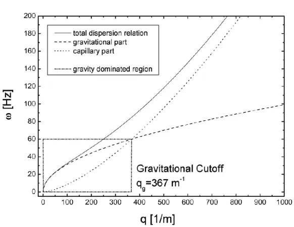
For wave vector numbers above the so-called gravitational cutoff qg the dis- persion properties are essentially caused by capillary forces, see Fig.2.2. Also important is the inverse relation between the gravitational cutoff and the sur- face correlation length `s [31, 27].
Another quantity of interest is the Hamiltonian function H in terms of eh and Ψ. By using the Fourier representation for Φ and the above mentionede expression forΦ, one finds the approximatione
∂Φ
∂z z=h
≈X
q
(qtanhqd)Ψ(q, t)e eiq·r, (2.11)
Figure 2.2: Dispersion relation of capillary gravity waves on a water surface at room temperature. For a surface tension of γ = 0.0727 Nm−1 and mass density of %l = 1000 kg/m3 the gravitational cutoff for water yields qg = 367 m−1.
which partially contributes to the kinetic energy density (2.4b). With (2.11) and the equations (2.5a), (2.5b) and (2.7), the Hamiltonian function (2.4a) yields
H = 1 2
X
q
X
q0
1
%lqtanhqdΨ(q, t)e Ψ(qe 0, t) + (%lg +γq·q0)eh(q, t)eh(q0, t)
× Z
A
d2rei(q+q0)·r. (2.12)
Due to the laterally periodic boundary conditions the allowed values for q and q0 are multiples of ±2π/L. Accordingly, the integral in (2.12) fulfills the orthogonality relation
1 A
Z
A
d2r ei(q+q0)·r =δ2(q+q0), (2.13) whereδ2(q+q0) = δ(qx+qx0)δ(qy+qy0) is a 2-dimensional delta function. With (2.13), one finally obtains the Hamiltonian for a system of decoupled harmonic
oscillators in the following form He = X
q
He h
Ψ(q),e eh(q) i
= 1 2AX
q
1
%lqtanhqd eΨ(q)
2 + %lg+γq2 eh(q)
2
. (2.14) In order to obtain the interfacial roughness σcw due to thermally excited capillary wave, h(q, t) is next treated as a random variable, which obeys the statistical requirements of ergodicity, spatial homogeneity and isotropy [32, 58].
In the statistical sense, the surface roughness can then be defined as the mean- squared deviation
σcw2 =hh(r, t)h(r, t)i=X
q
X
q0
heh(q, t)eh(q0, t)iei(q+q0)·r, (2.15) where the brackets denote an ensemble or time average, and the mean equi- librium height is located at hh(r, t)i = 0. According to the above statistical requirements forh(r, t), it follows thatσcw is independent of time and space, which implies the following conditions for the right-hand side of eq. (2.15) [58]
heh(q, t)eh(q0, t)i = heh(−q, t)eh(−q0, t)i= 0 (2.16) heh(q, t)eh(−q0, t)i = heh(−q, t)eh(q0, t)i=h
eh(q0)
2iδ2(q−q0). (2.17) Hence, the surface roughness, or correspondingly the interfacial widthσcw, can be evaluated from
σcw2 =X
q
h eh(q)
2i. (2.18)
The average valuesh eh(q)
2i perq−mode yield with eq. (2.14), (2.10) and the Maxwell-Boltzmann statistic the roughness expression perq−mode
h eh(q)
2i = RR
deh(q)dΨ(q)e |eh(q)|2 e−He(Ψ(q),ee h(q))/kBT
RR
deh(q)dΨ(q)e e−He(Ψ(q),ee h(q))/kBT
= R∞
0 deh(q)eh2(q) e−2kB TA (q2g+q2)eh2(q) R∞
0 deh(q) e−2kB TA (qg2+q2)eh2(q)
= kBT Aγ
1
qg2+q2 , (2.19)
wherekBis the Boltzmann constant. With (2.18), the capillary wave roughness can be expressed as a double sum over all q = (qx, qy) modes or alternatively
as a single sum overq =|q|, viz.
σ2cw=X
q>0
kBT Aγ
1
qg2+q2 . (2.20)
In (2.20) the summation starts from the lowest value q = 2π/L to the up- per cutoff qmax, which serves as truncation of the continuous (hydrodynamic model) medium. The upper cutoff is customarily estimated to be inversely proportional to the bulk correlation length [80], but it has also been taken to be inversely proportional to the intermolecular spacings [22, 99]. In the limit A→ ∞expression (2.20) yields the key formula of the capillary wave model:
σ2cw = kBT 2πγ
Z qmax
0
dq q
qg2+q2 = kBT 4πγ ln
1 + qmax2 qg2
. (2.21)
Eq. (2.21) can be derived from (2.20) by using the limit relation P
q>0 → A/(2π)2R
d2q. Due to the requirement of statistical isotropy, one can fur- thermore transform the integral into polar coordinates, which eventually leads to expression (2.21). The fraction qmax/qg may alternatively be replaced by 2π`s/`b, which describes the ratio between the short-range bulk and long-range surface correlation length. For temperatures far below Tc, a rough estimate for the bulk correlation length `b ≈ dm is commonly deduced from the mean molecular diameter dm [27, 22, 99]. Note that eq. (2.21) would lead to a log- arithmical singularity for the surface width, if the upper wave vector cutoff is not being introduced.
2.1.2 Effective Interface Hamiltonian
It may be readily seen that the interfacial roughness can effectively be de- termined by the potential energy of the Hamiltonian function eq. (2.4a). Ac- cordingly, one may derive the interfacial roughness at once by constructing an effective interface Hamiltonian H[h(r)], which describes the cost in en- ergy to deform the flat interface into a given rippled configuration. From this standpoint, one obtains the result of the previous section by constructing the so-called ”drumhead” Hamiltonian [39, 43]
Hdh[h(r)] = 1 2
Z
A
d2r 4% gh2(r) +γ Z
A
d2rq
1 +|∇kh(r)|2−1
, (2.22) which eventually yields with the following gradient expansion
q
1 +|∇kh(r)|2 = 1 + 1
2|∇kh(r)|2+O |∇kh(r)|4
. (2.23)
the ”capillary wave” effective Hamiltonian of Buff et al. [14, 8, 27, 80]
Hcw[h(r)] = 1 2
Z
A
d2r 4% gh2(r) + γ 2
Z
A
d2r |∇kh(r)|2. (2.24) Evidently, eq. (2.24) yields (regardless of the small difference 4% = %l −%v) the same statistical properties for liquid surfaces as eq. (2.4). By using the above formal approach, one can conveniently study a variety of surfaces by constructing the effective interfacial Hamiltonian of the system.
Effective interface Hamiltonians that yield in their normal coordinates a Gaussian form for the Maxwell-Boltzmann weighting factor, i.e. e−H[ee h(q)]/kBT, represent the class of Hamiltonians in the so-called Gaussian approximation.
Due to their simplicity and structural similarity with the capillary wave Hamil- tonian, these types of effective interface Hamiltonians play an important role in the statistical analysis of liquid surfaces. Among the most important phe- nomenological Hamiltonians in the Gaussian approximation is the Helfrich Hamiltonian, which is of the form [38, 24, 62]
HH[h(r)] = 1 2
Z
A
d2r4% gh2+1 2
Z
A
d2r n
γ|∇kh(r)|2+κ ∆kh(r)2o
, (2.25) where κ is the bending rigidity modulus. Helfrich’s Hamiltonian takes into account the curvature dependence of the surface energy, whereas the capillary wave Hamiltonian assigns the same surface energy to all configurations which have equal total area. In the normal mode representation eq. (2.25) can be arranged such that it resembles the effective capillary wave Hamiltonian, hence
HeHh eh(q)i
= 1
(2π)2 Z
d2q 1
2 4% g+γ(q)q2 eh(q)
2, (2.26) where now γ(q) denotes a q-dependent surface tension
γ(q) =γ +κq2, (2.27)
which reduces at large length scales, i.e. q → 0, to the macroscopic surface tension γ. Although the surface tension γ and the bending rigidity κ remain phenomenological constants, the Helfrich Hamiltonian makes the important prediction that the effectively measured surface tension is a function of length scales, i.e. 1/q.
Despite the fact that the phenomenological effective Hamiltonians uncover important properties of liquid vapor interfaces, such as long-range surface cor- relations belowTc, they fail to include bulk fluctuations or to provide a micro- scopic picture of the surface tension. In order to incorporate the predictions
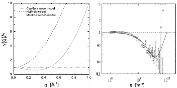
Figure 2.3: Surface tension as a function of q. Left: Comparison of Mecke- Dietrich’s model of surface tension (solid curve) with the phenomenological capillary wave theory (dotted curve) and the Helfrich theory (dashed curve).
The phenomenological Helfrich theory does not yield a specific value for κ/γ.
Here, it is chosen such that this ratio has the value of the one predicted by Mecke-Dietrich’s theory for largeq, i.e. κ/γ = 0.74CH2`2
b(1/2 + (`b/dm)2). The parameters are CH = 0.1, dm = 2˚A and `b = 5dm. Right: Experimental confirmation of the reduction of surface tension on a water surface at room temperature [30]. The solid curve has been obtained from Mecke-Dietrich’s theory for the parameters: CH = 0.35, dm = 10˚A and `b =dm/3 [23].
of the capillary wave model into the traditional Van der Waals model of in- terfaces, R. Evans formulated a density functional theory for inhomogeneous simple (mono molecular) liquids. The theory describes short-range density- density fluctuation in the bulk, as well as long-range surface fluctuation at a liquid-vapor interface [27, 28]. This approach was first adopted by M. Napi- orkowski & S. Dietrich [70] to construct an effective surface Hamiltonian which is based on a microscopic picture of the liquid. In a further improved version of the density functional approach, K. R. Mecke & S. Dietrich [63] derived an effective Hamiltonian that contains the capillary wave Hamiltonian as a limit result. Furthermore, it yields a q−dependent surface tension, which is essen- tially determined by the molecule diameterdm and the bulk correlation length
`b. After a subtle calculation, these authors obtain, in the Gaussian approxi-
mation, the following effective Hamiltonian in its normal mode representation HeM Dh
eh(q)i
= 1
(2π)2 Z
d2q 1 2
4% g 1−2CH(q`b)2
+γ(q)q2
eh(q)
2, (2.28) where the parameterCH is a weight for the curvature corrections of the density profile for thermally exited capillary waves. CH is limited between 0 < CH <
0.5, but it is not further specified in this theory. The surface tension γ(q) in eq. (2.28) decreases from its macroscopic value at q = 0 due to the effect of attractive long-range forces, reaches a minimum, and then increases ∝ q2 at large q, due to the distortion of the density profile when the surface is bent [62]. An approximate formula for the surface tension takes the form [63]
γ(q)
γ = 2−CH(q`b)2 ew(qdm)
(qdm)2 + 0.74CH2 1 2 +
`b dm
2
w(qde m)
! (q`b)2 + O (qdm)4
, (2.29)
with w(x) = 1e −(1 +x)e−x. In the limit q → ∞, Mecke & Dietrich’s theory predicted the following limiting expression for the surface tension [63]
γ(q→ ∞) = κ q2. (2.30) Eq. (2.29) holds in the so-called product approximation, which comprises the condition `b dm. However, it is argued that the maximum error in the product approximation is less than 10% even for `b ' dm [63, 69]. Expres- sion (2.29) yields the same limit result as the effective Helfrich surface tension (2.27), and eq. (2.29) reduces for (q`b)2 1 to the capillary wave result. A comparison between the three surface tension models is shown in Fig.2.3 (left).
The formation of a minimum in the surface tension appear to has been experi- mentally confirmed by surface sensitive X-ray scattering techniques for several liquids [30, 69, 50]. The experimental result for a water surface at room tem- perature is given in Fig.2.3 (right). It should be noted that the theoretically predicted and experimentally observed reduction in surface tension appears for relatively large q = (qx, qy) values (of the order 109m−1). Hence, if the maximum experimental q values are smaller than ca. 1/`b, one may readily use the capillary wave model. This will be in particular the case for X-ray reflectively experiments, where q is experimentally set to be zero. The same conclusion may be drawn from the effective Mecke-Dietrich Hamiltonian (2.28) for (q`b)2 1. In summary, the Mecke-Dietrich theory of surfaces appears to reveal some fundamentally new properties of fluid surfaces at atomic length scales, which is, however, up to now controversially debated in the scientific
community. With respect to time dependent surface properties, it should ac- knowledged that a time dependent density fluctuation theory for surfaces is not developed at the present time. Hence, the understanding of dynamic sur- face properties is ordinarily deduced from linear response theories of classical hydrodynamic [10, 53, 40, 41].
2.2 Surface Height Correlation Function
In comparison to surface microscopy techniques, such as Scanning Tunneling Microscope (STM) and Atomic Force Microscopy (AFM), surface sensitive X-ray scattering techniques provide statistical information from a relatively large surface area which can extend to several hundreds of square microns [99]. The statistical characterization of surface structures, in terms of height correlation functions, allow a relatively direct and systematic analysis of X-ray scattering data and play, therefore, a central role in the theoretical calculation of scattering cross sections from rough surfaces. In this section the static and dynamic height correlation functions are derived for some specific liquid surfaces, which are of interest for this work.
2.2.1 Static Height Correlation Function
The static height correlation function Czz(r,r0) describes the lateral correla- tion between two spatially separated height displacements on a surface. In analogy to the mean-squared roughness definition (2.15) one finds for the height correlation function
Czz(r,r0) =hh(r, t)h(r0, t)i=X
q
X
q0
heh(q, t)eh(q0, t)iei(q·r+q0·r0), (2.31) Based on the demanded statistical properties for the random height displace- ments h(r, t) (see section 2.1.1) it follows with eq. (2.16) and (2.17) that the height correlation function is spatially only a function of the separationr0−r.
Hence, eq. (2.31) becomes
Czz(r0−r) =X
q
h|eh(q)|2ieiq·(r0−r). (2.32) In addition to the spatial dependence, eq. (2.31) and (2.15) require the follow- ing two general properties
Czz(r0−r) = Czz(r−r0), (2.33) σ2 = Czz(r0−r)
r0−r=0, (2.34)
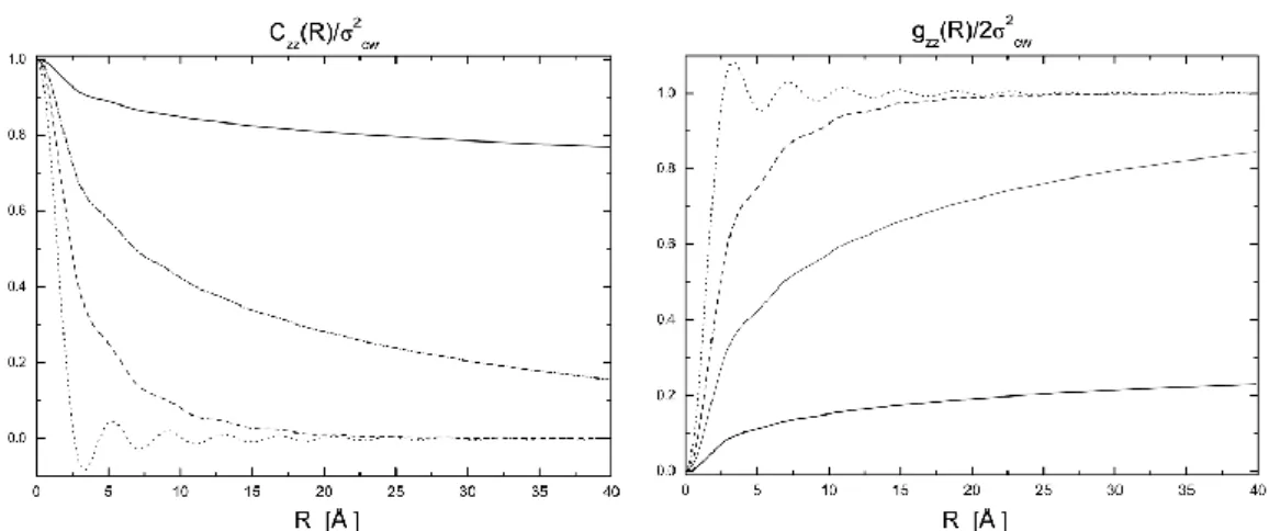
Figure 2.4: Normalized static height correlation functionCzz(R)/σcw2 as a func- tion ofR. Left: Normalized height correlation for a water surface at room tem- perature (solid line); the correlations lengths are `s = 2.7mm and `b ≈ 2rm, with the mean molecular radius rm(H2O) = 1.92˚A [11]. The qmax cutoff, in- herent to the capillary wave model, is taken to be qmax = 2π/`b. The height correlation decays as the surface correlation length decreases; three arbitrary cases are illustrated: qg =qmax/100 (dash-dotted line), qg =qmax/10 (dashed line) andqg =qmax (dotted line). Right: Illustration of the normalized height- difference correlation function for the same values used in the left plot.
where the condition (2.34) defines the maximum value for height correlation function. In the continuous limit, expression (2.32) transforms into the integral expression
Czz(R) = 1 (2π)2
Z
d2q Cezz(q)eiq·R, (2.35)
whereR=r0−randCezz(q) is the reciprocal space height correlation function, which takes for the capillary wave model the following form
Cezz(q) = kBT γ
1
q2+qg2. (2.36)
The real space expression for the height correlation function can be evaluated
by transforming integral (2.35) into polar coordinates, which yields Czz(R) = kBT
2πγ
Z qmax
0
dq q
q2+qg2 J0(qR), (2.37)
= kBT 4πγ
qmax qg
2
×
∞
X
k=0
(−1)k Γ[1 +k]2F1h
1,1 +k; 2 +k;−qmax2 /q2gi qmaxR
2 2k
, (2.38) where R = (x2 +y2)1/2, and J0(qR) represents the Bessel function of the first kind. By performing the integral (2.37), with the sum representation for the Bessel function [33], one finds the result (2.38), where 2F1[1,1 +k; 2 + k;−q2max/qg2] is the regularized hypergeometric function and Γ[1 +k] is the Gamma function. Eq. (2.38) does satisfy the symmetry condition (2.33) as well as
σ2cw=Czz(R)
R=0. (2.39)
Note that the sharp cutoff in (2.37) leads to oscillation in the height correlation function, see Fig.2.4. Another quantity, that is of interest in the calculation of scattering cross sections from surfaces is the static height-difference correlation functiongzz(R) [90]:
gzz(r0−r) =D
h(r0, t)−h(r, t)2E
, (2.40)
which can easily be reduced to the radial height-difference correlation function for liquid surfaces
gzz(R) = 2 σcw2 −Czz(R)
. (2.41)
The spatial behavior of the radial height correlation function (2.38) and the height-difference correlation function (2.41) are illustrated in Fig.2.4.
It is worth mentioning that the commonly used height correlation function is derived from (2.37) for the limit qmax→ ∞ [81, 6, 22, 99]. In that case one finds [33]
Czz(R) = kBT 2πγ
Z ∞ 0
dq q
q2+q2g J0(qR), (2.42)
= kBT
2πγK0(qgR), (2.43)
where K0(qgR) is the modified Bessel function of the second kind. The rela- tively simple result of eq. (2.43) has some useful properties with regard to the calculation of scattering functions, see section 3.2. However, due to the limit
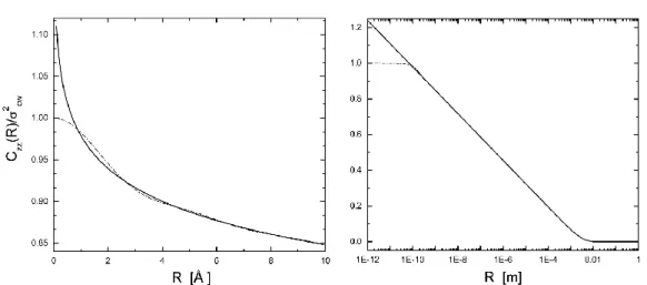
Figure 2.5: Normalized static height correlation function Czz(R)/σcw2 as a function ofR. Comparison between eq. (2.43) (continuous line) and eq. (2.38) (dash-dotted line). The normalized height correlation functions are obtained by using the material constants for water at room temperature. qmax is taken to be qmax = π/rm, where rm = 1.92˚A. Left: For short distances, the main difference appears atR = 0. Right: In the limit R `b, eq. (2.43) is in good agreement with the exact solution for the height correlation function (2.38).
limR→0K0(qgR)→ ∞ the condition (2.39) is obviously not satisfied and, cor- respondingly, the theoretical scattering functions that are derived from (2.43) contain singularities in reciprocal space. A comparison between eq .(2.38) and (2.43) is shown in Fig.2.5.
2.2.2 Dynamic Height Correlation Function
The static height correlation functions of the previous section are only applica- ble to static scattering experiments from liquid surface. In time resolved (sur- face sensitive) experiments such as dynamical light scattering (DLS), or X-ray intensity correlation spectroscopy (XICS), the measured quantity is, however, related to the dynamic height correlation function, which is in general defined as
Czz(r,r0, t, t0) =hh(r, t)h(r0, t0)i. (2.44) With the statistical properties of the height displacement function h(r, t), see section 2.1.1, the autocorrelation functionCzz(r,r0, t, t0) reduces to a function which depends only on spatial and time differences [58, 32]. Accordingly, the dynamic height correlation function can, henceforth, be written as
Czz(r0−r, t0−t) =hh(r, t)h(r0, t0)i, (2.45)
and, moreover, it obeys the following conditions
Czz(r0−r, t0−t) = Czz(r−r0, t−t0), (2.46) Czz(r0−r) = Czz(r0−r, t0−t)
t0−t=0, (2.47) σ2 = Czz(r0−r, t0−t)
r0−r=0,t0−t=0. (2.48) In order to obtain a specific expression for the dynamic height correlation function, it will be useful to use the Wiener-Khintchine theorem, which relates the autocorrelation function of stationary random processes and the power spectrum of these fluctuations, by a conventional Fourier transform [58]. Using the Wiener-Khintchine theorem in combination with eq (2.35), one can derive the dynamic height correlation function from
Czz(R, τ) = 1 (2π)3
ZZ
dω d2q Szz(q, ω)ei(q·R−ωτ), (2.49) where R=r0 −r, τ =t0−t and Szz(q, ω) represents the power spectrum of thermal surface displacements.
Explicit expressions for the surface spectrum Szz(q, ω) have been deduced from linear response theory by several authors [10, 53, 40, 41]. In the limiting case of deep liquids, as considered in this work, the surface spectrumSzz(q, ω) for an incompressible fluid with arbitrary viscosity is given by
Szz(q, ω) = 2kBT ω Im
q/%l
ω2s(q)−(ω+i2νq2)2−4ν2q4(1−ω/νq2)1/2
, (2.50) where ν is the kinematic viscosity. The depth dependance is in The Fourier transform of eq. (2.50) is a nontrivial task and, therefore, it is only solved below for special cases. For a highly viscous liquid eq. (2.50) can be approximated by a Lorentzian curve, which peaks atω= 0 with a half width at half maximum (HWHM) of Γh(q) = γq/(2ν%l). In the low viscosity case the surface spectrum yields two equally spaced sharp peaks atω=±ωs(q) with a HWHM of Γl(q) = 2νq2. Here the subscribesh and l denote the limits for high and low viscosity liquids, respectively.
A. Height correlation function for low viscosity liquids
In the low viscosity limit the general surface spectrum eq. (2.50) simplifies to [41]
Szz(q, ω) = 2kBT q
%l
2Γl(q)
(ω2−ω2s(q))2+ (2ωΓl(q))2 , (2.51) with
Γl(q) = 2νq2. (2.52)
The above expression can be used to derive the height correlation function of propagating capillary waves. By performing the Fourier transform with respect toω we find [33]
Cezz(q, τ) = kBT γ
1
q2+qg2 e−Γl(q)τ
"
cos
ωs(q)τ q
1−(Γl(q)/ωs(q))2
+ Γl(q)
ωs(q) q
1−(Γl(q)/ωs(q))2 sin
ωs(q)τ
q
1−(Γl(q)/ωs(q))2 #
,
(2.53) where we used the trigonometric relations sin(arccosα) = (1 − α2)1/2 and sin 2α = 2 sinαcosα. A useful approximation is obtained, if the condition Γl(q)/ωs(q)1 is satisfied in the range of experimental wave vector transfers.
Eq. (2.53) then simplifies to Cezz(q, τ)≈ kBT
γ 1
q2+qg2 cos (ωs(q)τ)e−Γl(q)τ, for Γl(q)/ωs(q)1. (2.54) For the discussion of surface sensitive XICS the reciprocal space expression (2.54) is in fact sufficient enough, as will be shown later. Note that the solutions (2.53) and (2.54) hold only forτ ≥0. The corresponding real-space expression to (2.54) can be expressed in a series form; however, its usability is questionable and, therefore, it is left out of the discussion.
B. Height correlation function for high viscosity liquids
For a liquid with high viscosity the surface spectrumSzz(q, ω) takes the form of a Lorentzian curve, viz.
Szz(q, ω) = 2kBT 1 γq2
Γh(q)
ω2+ Γ2h(q) 1 +qg2/q22 , (2.55) where
Γh(q) = γ
2ν%l q . (2.56)
The half width at half maximum is essentially determined by Γh(q) and addi- tionally broadened by a term that contains the gravitational cutoff. For typical experimental q−values, the contribution of qg gives a negligible correction to the width of Szz(q, ω) and is, therefore, often omitted [41]. With the surface
spectrum (2.55) one can easily calculate the height correlation function for high viscosity liquids, which yields [33]
Cezz(q, τ) = kBT γ
1
q2+qg2 e−Γh(q)τ(1+q2g/q2), for τ ≥0. (2.57) It is worth noting that eq. (2.54) and (2.57) reduce to the static height corre- lation function for τ = 0, i.e. they obey the condition (2.47).
Elastic X-Ray Scattering From Rough Surfaces
The interaction of electromagnetic waves with material interfaces is a classical discipline in scattering theory. Among the first descriptions one may count Snell’s law of refraction and the Fresnel formulas of reflection and transmission, which apply to the interaction of electromagnetic waves at a perfectly smooth surface [9]. Since these classical works of Snell and Fresnel, the analysis of surface scattering from smooth, structured and rough surface has been the object of theoretical and experimental studies of a large body of work, which contains the description of surface scattering of long wavelength radar waves, visible light, down to X-ray wavelengths [7, 5, 104, 99, 22].
With the growing number of X-ray synchrotron radiation sources, surface scattering has been rediscovered as a powerful experimental tool and increas- ingly used to investigate surface properties, down to the atomic-scale. For X-ray wavelengths, the interaction of electromagnetic wave with matter is mainly determined by the electron charges in the scatterer. Although there are many phenomena associated with the interaction, here we will only con- sider those related to elastic Thompson scattering. Since we are not concerned with absorption and emission processes, the quantum theory of photon-electron scattering will not be needed and, hence, the scattered intensity expressions can be readily obtained from Maxwell’s field equations.
In this section, we will relate the statistical properties of rough surface to the scattered X-ray intensity. The scattering process will henceforth be describe within the scalar theory of electromagnetic wave scattering. In view of the discussion on quasi-elastic scattering, some of the derivations and results in this chapter will later serve us as a reference.
3.1 Basic Principles
According to the classic description of scattering, one can determine the scat- tered intensity from the modulus square of the scattered electric field. In order to derive the explicit expression for the scattered electric field, we will consider throughout this work a nonmagnetic, isotropic and homogenous scatterer. In that case, the propagation of the electric field can be described by the (scalar) Helmholtz equation [9], namely
∆Ue(r, ω0) +k20n2(r, ω0)Ue(r, ω0) = 0 . (3.1) wherek0 is the free-space wave number and ω0 is the frequency of the field at the observation point r = (r, z) with r = (x, y). U(r, ωe 0) is a complex scalar representation for the electric field and n(r, ω) is the refractive index, which characterizes the optical properties of scatterer in the occupied volume V as well as the exterior volume VR, such as n(r, ω0) = 1 takes the vacuum value for r ∈ VR. To specify the response characteristics of the index of refraction in the hard X-ray limit, it is sufficient to use the classical formulas, viz.
n2(r, ω0) = 1 + 4πχ(r, ω0) , for r ∈V (3.2) where, in the Drude model [42], the dielectric susceptibilityχ(r, ω0) is described as
χ(r, ω0) =rec2NX
j
fj
ω2j −ω02−iγjω0. (3.3) In eq. (3.3) the constants re and c represent the classical electron radius and the speed of light, respectively. N is the number of molecules per unit volume with Z electrons per molecule. The resonance frequencies ωj of the electrons are weighted by the oscillation strengthfj, which gives the number of electrons per resonance frequency and, thus, fj obeys the sum rule Σjfj = Z. γj is a phenomenological damping constant [42]. For X-ray frequencies far beyond any resonance frequency one finds for (3.2)
n2(r, ω0) = 1−4πreρ(r)c2
ω20 , (3.4)
which simplifies, with the expansion √
1−x≈1−x/2, to the form
n(r, ω0) = 1−δ(r, ω0) , (3.5) with
δ(r, ω0) = 2πreρ(r)c2
ω20 . (3.6)
Here ρ(r) is the number of electrons per unit volume. The dispersion term δ(r, ω0) is zero in vacuum and is, otherwise, a small positive quantity of the order of 10−6 (for X-ray wavelengths). Due to the negative sign in (3.5), the index of refraction in matter is always smaller than in vacuum. Hence, at grazing incident angles below the critical angle αc ≈ p
2δ(r, ω0), the nega- tive sign leads to the phenomenon of external total reflection in contrast to the analogous phenomenon of total internal reflection for visible light [99].
Corrections to expression (3.5) contain an addition absorption term β(r, ω0), and the proper atomic scattering factor fp = fp0 +fp0(ω0) +ifp00(ω0) of each componentp of the scattering material, so that in general, n(r, ω0) yields the expression [99]
n(r, ω0) = 1−δ(r, ω0) +iβ(r, ω0), (3.7) with the dispersion and absorption terms
δ(r, ω0) = 2πreρ(r)c2 w20
X
p
fp0+fp0(ω0)
Z , (3.8a)
β(r, ω0) = 2πreρ(r)c2 w20
X
p
fp00(ω0)
Z = c
2ω0µ(r) , (3.8b) whereµ(r) represents the linear absorption length.
Next we will give the formal solution for the electric field in a scattering experiment. The finding of a rigorous solutions for the Helmholtz equation including the proper boundary conditions is a classic problem in diffraction optics and, generally, a difficult mathematical task [93]. A simpler and widely accepted approach to the solution of (3.1) is based on integral equations for U(r, ω). In order to derive the needed integral equations it will be useful toe express eq. (3.1) in form of Schr¨odinger’s equation
∆Ue(r, ω0) +k20Ue(r, ω0) =−4πFe(r, ω0)Ue(r, ω0) , (3.9) where
Fe(r, ω0) = ω02
c2 χ(r, ω0), (3.10)
is called the optical potential of the medium. The wave number k0 is repre- sented in (3.10) by ω0/c =k0. For values r ∈ VR the optical potential obeys the conditionFe(r, ω0) = 0, which is in accordance with the demanded vacuum value for the index of refraction outside of V, see Fig.3.1. The Green’s func- tion G(r,r0, ω0) associated with the Helmholtz operator (∆ +k02) satisfies the equation
(∆ +k02)G(r,r0, ω0) =−4πδ3(r−r0). (3.11)
Figure 3.1: Illustration of the notation for potential scattering expressions and surface scattering expressions (Kirchhoff integral formulation). The exterior volume VR is for simplicity definition by a sphere SR of radius R (note, that V * VR). The arbitrary volume V can coincide either with the volume V or with VR. The volumes V, V and VR are respectively bounded by the surfaces S, S and SR. The normal unit vectors n, nS and nR point outwards to the surfaces S, S and SR, respectively.
By using Green’s integral theorem and eqs. (3.9) and (3.11) one finds the fol- lowing integral equation [103]
Z
V
Ue(r0, ω0)δ3(r−r0)d3r0 = Z
V
G(r,r0, ω0)Fe(r0, ω0)U(re 0, ω0)d3r0
− 1 4π
Z
S
"
Ue(r0, ω0)∂G(r,r0, ω0)
∂nS −G(r,r0, ω0)∂Ue(r0, ω0)
∂nS
# dS, (3.12) where the volume V coincides either with the volume V or with VR. The derivatives ∂/∂nS denote differentiations along the outward normal to the surfaceS, which bounds the domain V. Depending on the choice of domainV and position of the observation pointr one obtains four possible solutions for

![Figure 3.4: Left: Theoretical reflectivity curves for CH 3 − [CH 2 ] 1 8 − CH 3 at T = 130 ◦ C](https://thumb-eu.123doks.com/thumbv2/1library_info/3684479.1505173/53.892.158.738.179.599/figure-left-theoretical-reflectivity-curves-ch-ch-ch.webp)