𝐷𝐾 and 𝜋𝜋 Scattering from Lattice QCD
DISSERTATION ZUR ERLANGUNG DES DOKTORGRADES DER NATURWISSENSCHAFTEN (DR. RER. NAT.) DER F A K U L T Ä T F Ü R P H Y S I K
DER UNIVERSITÄT REGENSBURG
vorgelegt von
Antonio Cox
aus
London, Vereinigtes Königreich
im Jahr 2018
Promotionsgesuch eingereicht am: 15.12.2017 Arbeit wurde angeleitetvon: Prof. Dr. A. Schäfer
Prüfungsausschuss: Vorsitzender: Prof. Dr. F. Gießibl 1. Gutachter: Prof. Dr. A. Schäfer 2. Gutachter: Prof. Dr. V. Braun weiterer Prüfer: PD Dr. J. D. Urbina
Termin Promotionskolloquium: 19.12.2018
Introduction 5
1 Relativistic scattering 7
1.1 The S-matrix . . . 8
1.1.1 Symmetries of theS-matrix . . . 10
1.2 Particle states . . . 12
1.2.1 Vacuum and one-particle states . . . 12
1.2.2 n-particle states . . . 13
1.2.3 The full space . . . 16
1.3 Relativistic scattering . . . 19
1.3.1 Poincaré invariance of the S-matrix . . . 19
1.3.2 Two particle scattering . . . 20
1.3.3 Crossing . . . 23
1.4 Causality, analyticity, unitarity . . . 25
1.4.1 Causality implies analyticity . . . 25
1.4.2 Unitarity . . . 26
1.4.3 Partial wave amplitudes, phase shifts . . . 29
1.4.4 Threshold behaviour, bound states, resonances . . . 32
1.4.5 Potential . . . 35
2 QCD on the continuum and on the lattice 41 2.1 Continuum QCD . . . 42
2.1.1 The classical action . . . 42
2.1.2 Quantisation and the QCD Hilbert space . . . 44
2.1.3 The quark model for mesons . . . 46
2.2 QCD on the lattice . . . 47 1
2.2.1 The pure gluonic action . . . 47
2.2.2 The Wilson fermionic action . . . 49
2.2.3 Path integral quantisation on the lattice . . . 52
2.2.4 The lattice Hilbert space and the spectral decomposition . . . 55
2.3 Lattice methods . . . 62
2.3.1 Quark field smearing . . . 62
2.3.2 Stochastic sources . . . 64
2.3.3 The variational method . . . 67
2.4 Extracting scattering data from lattice simulations . . . 70
2.4.1 Lüscher’s method . . . 70
2.4.2 The potential method . . . 74
3 DK and D∗K scattering from lattice QCD 77 3.1 Overview of the problem . . . 77
3.1.1 The physical picture . . . 77
3.1.2 Finite volume considerations . . . 78
3.2 Finite energy extraction . . . 81
3.2.1 Lattice setup . . . 81
3.2.2 Operator basis and the correlator matrix . . . 81
3.2.3 Wick contractions . . . 82
3.2.4 Stochastic sources insertion . . . 85
3.2.5 Technical implementation . . . 87
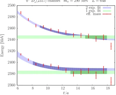
3.2.6 Energy results . . . 89
3.3 Connection to infinite volume . . . 94
3.3.1 Phase shift . . . 95
3.3.2 Potential . . . 100
3.3.3 Final spectrum and comparison to experiment . . . 103
3.4 Decay constants . . . 106
4 ππ and Kπ scattering 111 4.1 Introduction . . . 111
4.1.1 Experimental overview . . . 111
4.1.2 Lattice implementation . . . 112
4.2 Results . . . 114
4.2.1 Phase shifts . . . 114
4.2.2 Comparison with other results . . . 116
Summary 119 A Appendix 121 A.1 Some group theory . . . 121
A.1.1 Cosets, orbits and little groups . . . 121
A.1.2 Subduced and induced representations . . . 123
A.1.3 The Lorentz group . . . 125
A.1.4 The Poincaré group and its unitary irreducible representations . . . 129
A.2 Space-time discretisation . . . 133
A.3 Evaluation of the Ds←→DK diagrams . . . 136
Bibliography 139
Lattice QCD simulations have the capability to render precious information about various non-perturbative aspects of QCD which would otherwise be unknown to us. Among these aspects, the properties of scattering of relativistic particles - namely phase shifts, scattering lengths, resonance couplings etc. - play a central role.
At first sight, lattice QCD may not seem a suitable framework to handle scattering. As the theory is defined on a finite discrete Euclidean space-time, it is not possible to introduce the notion of asymptotic states. Particles can never be isolated and will always feel the effect of each other due to the presence of the boundary. Consequently, a scattering formalism together with the features that result cannot be introduced. No scattering happens on the lattice.
Fortunately, the lack of a scattering formalism in Lattice QCD does not prevent us from accessing, from lattice simulations, the collision properties of particles of our real world.
The outstanding relations introduced by Lüscher and subsequently generalised by others, determine a connection between the energies on the lattice and the scattering matrix of the infinite volume quantum field theory. If the systematics are kept under control, results can be compared to experiment.
The task of this work is to employ Lüscher’s method for studying the elastic scattering in four different channels, DK, D∗K, ππ and Kπ, in the JP = 0+, 1+, 1− and 1− sectors, respectively. In the first two channels the enigmaticD∗s0(2317) andDs1(2460) bound states are respectively present, while the last two couple to the ρand K∗ resonances.
The thesis is presented in an approximately self-contained fashion. Many of the formulae and features which are concretely applied in chapters (3) and (4) to the channels under consideration are defined and discussed in general in the supporting chapters (1) and (2).
Specifically, relativistic scattering theory is the topic of chapter (1). Starting from basic principles, as Poincaré invariance, asymptotic completeness and analyticity of theS-matrix, the whole theory can be constructed in a general way. Concepts such as phase shifts and
5
resonances in the relativistic setting appear as a consequence and are also treated. In chapter (2) some general features of continuum QCD and lattice QCD are discussed. The way Lüscher’s formalism connects lattice data to physical scattering information is presented in detail at the end of the chapter. The scattering parameters of the DK and D∗K system as well as the mass, the coupling and the decay constants of the D∗s0(2317) and Ds1(2460) states are calculated and discussed in Chapter (3). Finally, in chapter (4), the results for the masses and widths of the ρ and K∗ resonances and their coupling to the channels ππ and Kπ are presented.
Relativistic scattering
Since Lüscher has extended the window of applications of lattice simulations from isolated particles to scattering states, many of the notions inherent to scattering theory have become widely used in the lattice community. It is today possible to address on the lattice questions such as “what is the decay width of the ρ resonance?”, or “what is the threshold behaviour of neutron-proton scattering and is this behaviour compatible with the existence of a bound state?”. Due to the significant role played for the lattice, this chapter is dedicated to the theory of relativistic scattering and to some of its notions relevant for this work.
Relativistic scattering theory is based on general, non-perturbative and model independ- ent principles which are shared by any reasonable relativistic quantum field theory. A rigor- ous treatment is not required here and the assumptions listed in the following by no means constitute a formal set of mathematical postulates1. With this clarification, we require that:
• The space of states is a separable Hilbert space H in which the laws of quantum mechanics apply.
• The Hamiltonian is such that the system behaves freely at asymptotic times t→ ±∞
and the space enjoys the property of asymptotic completeness.
• The Poincaré group is a symmetry of the theory, i.e., the Hilbert space carries a unitary representation U(a,Λ) of the Poincaré group. The spectrum of the four-momentum operatorPµ spans the space and lies in the forward light cone, P2 ≥0 and P0 ≥0.
• There exists a unique state, the vacuum|0i, which has unit norm and is invariant under Poincaré transformations, U(a,Λ)|0i=|0i, as well as a set of stable particles (mi, si)
1Readers interested in a formal definition may refer to those applications of constructive quantum field theory where a rigorous axiomatic formulation is attempted.
7
which transform irreducibly from which, the whole Hilbert space can be constructed by tensor products.
• A field theoretical description on Minkowski spacetime can be given. In particular, observables commute for space-like distances (causality),
[O1(x), O2(y)] = 0, (x−y)2 <0.
The first two assumptions are at the base of a general scattering theory and are discussed in Sec. (1.1). The second two specialise to relativistic scattering and introduce the concept of relativistic particle states. These will be discussed in Sec. (1.2). The field description is actually not required in this chapter but was added for completeness. Instead, in Sec. (1.4), the additional assumption of analyticity of theS-matrix - in the sense that will be explained - will be added.
The topics covered in this chapter can be found in several textbooks, see e.g. Refs. [1–5].
1.1 The S-matrix
As quantum field theory is a particular case of a quantum mechanical theory, the same laws of quantum mechanics apply. In particular, a Hamiltonian operator is present in the Hilbert space H of the theory. The dimensionality of the latter is not finite, although the notion of separability is required, i.e. a countable orthonormal basis is present. Nevertheless, we will not be concerned with mathematical formalities and non-normalisable states will be extensively considered.
Concerning time evolution, we will work in the Heisenberg picture, where operators are time-dependent and state vectors are constant. The second condition above assumes that at asymptotic times t→ ±∞ the Hamiltonian of the quantum theory is such that the system behaves freely. In ordinary quantum mechanics, the existence of this freedom can be proved for potentials (in the coordinate representation) going to zero fast enough as the coordinate tends to infinity. In a quantum field theory, such a behaviour must be postulated. We are in the setting of a scattering experiment: at time t→ −∞, long before the collision, a system of isolated and non-interacting particles are prepared and will undergo scattering at finite times. Similarly, long time after the collision takes place, the particles no longer interact and behave freely. At this stage, it is irrelevent whether the states have a particle interpretation and the content of this subsection can be applied in general.
Due to the freedom at asymptotic times, “in” states and “out” states can be naturally introduced: |φ,ini and |ψ,outi are states which are non-interacting in the infinite past and infinite future, respectively. As the Heisenberg picture is being considered, please note that e.g. the state|φ,ini describes the whole history of the system, also when the interaction is over, and the label “in” just reminds one that at t→ −∞ the system was free.
The asymptotic completeness assumption states that in-states and out-states both span the physical Hilbert space. This means that it is possible to find in H two complete ortho- gonal bases2
X
a
1 fa
|a,ini ha,in|=1, ha,in|a0,ini=qfafa0δaa0, (1.1.1)
X
a
1
fa|a,outi ha,out|=1, ha,out|a0,outi=qfafa0δaa0. (1.1.2) The sums run over the eigenvalues of a complete set of commuting operators. |a,ini is a state such that a simultaneous measurement of such operators performed att → −∞, when the system is free, will result in the set of values “a”. At a later time, the measurament of the same observables will lead in general to a different result, as the eigenstates of the evolving operators corresponding to the eigenvaluesa will have evolved. Similarly, the state
|a,outi is labelled by the result of a measurement performed at t→ ∞.
The S-matrix, or the scattering matrix, is defined to be the operator S that maps the out-states onto the in-states,
|ψ,ini = S|ψ,outi. (1.1.3)
It is unitary,
SS†=S†S =1, (1.1.4)
as it can be seen using Eqs. (1.1.1) and (1.1.2):
1=X
a
1
fa|a,ini ha,in|=SX
a
1
fa|a,outi ha,out|S†=SS†. (1.1.5) The unitarity of theS-matrix will have profound consequences, as we will see.
Suppose that the physical state is |a,ini. By the laws of quantum mechanics, the prob- ability amplitude that a measurement at timet→ ∞will result in “a0” is given by (fafa0)−12
2The annoying normalisation factorsfa=ha|aiare shown to make contact to the relativistic normalisation that will be used.
times
ha0,out|a,ini=ha0,in|S|a,ini=ha0,out|S|a,outi=Sa0a,
which are the matrix elements of the operator S in either basis. The unitarity of S is just a conservation of probability - the probability that at time t → ∞ |a,ini will be found to be in any state is one:
X
a0
1 fa0fa
|Sa0a|2 = X
a0
1 fa0fa
| ha0,in|S|a,ini |2 =X
a0
1 fa0fa
ha,in|S†|a0,ini ha0,in|S|a,ini
= 1
faha,in|S†S|a,ini= 1
fa ha,in|a,ini= 1. (1.1.6) If S = 1, no interaction takes place in the theory, or |a,outi = |a,ini for any a. It is customary to separate the non-trivial part of S from the T-matrix term which is due to interaction:
S = 1 +iT, Sa0a
√fa0fa =δa0a+i Ta0a
√fa0fa
. (1.1.7)
Unitarity SS† = 1 implies 1
i
T −T†=T T†, 1
i (Ta0a−Taa∗0) =X
a00
1
fa00Ta0a00Taa∗00. (1.1.8) The lhs is called the absorptive part and would be twice the imaginary part of Ta0a if, for some reason,Ta0a =Taa0. This happens for instance for elastic scattering of spinless particles or if time reversal is a symmetry of the theory. In this case,
2ImTa0a =X
a00
1
fa00Ta0a00Taa∗00. (1.1.9) In particular, taking a=a0,
2ImTaa =X
a00
1
fa00|Taa00|2. (1.1.10) These formulas are different versions of what in the literature is known as the optical theorem.
1.1.1 Symmetries of the S-matrix
Suppose there is an observable X that commutes with the S-matrix, [X, S] = 0. Then clearly, if the initial state|a,iniis an eigenstate of X with eigenvaluex,X|a,ini=x|a,ini,
so will beS|a,ini:
X(S|a,ini) =SX|a,ini=x(S|a,ini). (1.1.11) Thus, final states|a0,outishould be looked for only in the subspace relative to the eigenspace xand the latter is referred to as a good quantum number. In terms of scattering of particles, the collision will not alter the result of the measurement of the observableX. From now on, the labels “in/out” will be dropped with the understanding that all considerations are valid for both cases.
Suppose now that there is a group G and a representation D acting on the Hilbert space such that [Dg, S] = 0 for all g in G. By Schur’s lemma, the S-matrix is diagonal if sandwiched by elements of an irreducible representation of the group and does not depend on the particular elements of the representation space. To be specific, suppose we choose our basis asa= (x, cx, µ), wherexidentifies the irreducible representation ofG,cx labels its vectors andµare the remaining indices to completely identify the state. Then, theS-matrix simplifies to
hx0c0xµ0|S|x cxµi=Sx0c0xµ0,xcxµ =δxx0δcxc0xSµx0µ, (1.1.12) where the non trivial part Sµx0µ is a function of the irreducible representation labelled by x. Thus, to exploit this symmetry, it is convenient to choose a basis for the Hilbert space according to irreducible representations of the symmetry group. If we had chosen another basis, labelled say byb = (y, µ), a change of basis could have been performed,
|bi=|y µi=X
xcx
gxcy x|x cxµi (1.1.13) and theS-matrix element with respect to the original basis could have be expanded,
hy0µ0|S|y µi = X
xx0
X
cxc0x
gxy00c∗0xgxcy xhx0c0xµ0|S|x cxµi
= X
xx0
X
cxc0x
gxy00c∗0xgxcy
xδxx0δcxc0xSµx0µ =X
x
X
cx
gyxc0∗
xgyxc
x
!
Sµx0µ
= X
x
hyx0ySµx0µ. (1.1.14)
For fixedµµ0, theS-matrix elementhy0µ0|S|y µiis a sum over irreducible componentsSµx0µ. Partial wave decompositions, both in ordinary quantum mechanics and in quantum field theory, are typical examples of Eq. (1.1.14). In our context, the symmetry groups will include the Poincaré group as well as internal symmetries as isospin.
1.2 Particle states
Up to this point we have considered a quantum mechanical theory equipped with a unitary S-matrix operator in the Hilbert space. We now want to add the condition of relativistic invariance, i.e., we want to implement in the theory the well established fact that physics is the same in all inertial frames of reference. The transformation between frames is enforced by the Poincaré action x → Λx+a on Minkowski spacetime, leaving the distance ds2 = ηµνdxµdxν invariant.
In the quantum mechanical setting, this symmetry is represented by requiring that the action of the Poincare transformation on the Hilbert spaceHvia an operatorU(g)≡U(a,Λ) is such that measurable quantities are unchanged,
|hψ0|φ0i|=hψ|U†(g)U(g)|φi=|hψ|φi|. (1.2.1) This means that, for anyg,U†(g)U(g) = eiφ1for some phaseφ. Moreover, any subsequent transformation should imply U(g0g) = eiφU(g0)U(g). The phase factors can be set to
±1 without loss of generality, so that the operators are either unitary or anti-unitary and representations may be double-valued. Quantum-mechanically, one considers the universal cover of the Poincaré group so that operators are unitary and representations are single- valued.
Then, the Hilbert space H must carry a (reducible) unitary representation
U(a,Λ) =eiaµPµe−2iωµνMµν, (1.2.2) where Pµ and Mµν are meant to be operators on H satisfying the Poincaré algebra, Eqs.
(A.1.15) and (A.1.21). The Hamiltonian operator H is identified with P0, P is the three- momentum operator and the Mµν includes the angular momentum J operator. Let us now look at the states in the Hilbert space.
1.2.1 Vacuum and one-particle states
First of all, we assume the existence of a unique vacuum state |0i ≡ |0,ini = |0,outi with unit norm which is associated to the trivial irreducible representation and which is invariant under U(a,Λ), U(a,Λ)|0i = |0i. This implies that |0i is annihilated by the generators, Pµ|0i= 0 andMµν|0i= 0 and hence has zero energy.
Secondly, we require that there are subspaces of H, say N of them, that transform
irreducibly under the Poincaré group. More precisely, for eachi= 1, ..., N there is a positive3 numbermiand a non-negative integer or semi-integersi which identify the smallest subspace H(mi,si) ⊂ H made of all those states |misi; ψi on which the Casimir operators P2 and W2, built from the algebra in Eq. (1.2.2), assume the same value m2i and −m2isi(si+ 1), respectively. A basis |misi;piσii of H(mi,si), with scalar product given by (A.1.38), is labelled by the eigenvalues pi ∈ R3 and σi = −s, ..., s of respectively P and Σ, where Σ is some operator constructed from the algebra and commuting with P2, W2 and P. As discussed in App. (A.1.4), H(mi,si) is an irreducible space of the Poincaré group and the action of the general element Eq. (1.2.2) on H(mi,si) is given by Eq. (A.1.36).
We see that the concept of relativistic particle emerges automatically once we include the Poincaré group in our quantum mechanical theory. Indeed to the couple (mi, si) we associate a particle with mass mi and spinsi, which are identified simply by the constant eigenvalues of P2 and W2 respectively when acting on H(mi,si). The degrees of freedom of the particle are instead provided by the operators P, P0 = H (redundant) and Σ, whose eigenvalues on H(mi,si) identify respectively the three-momentum pi, the energy Ei =qm2i +|pi|2 and the spin degeneracy σi of the particle. Σ can be chosen such that it reduces to J3 in the centre of mass frame (the standard or canonical basis), the component of the angular momentum along the z-axis, leading to the usual non-relativistic interpretation of spin4. Another common choice is to take Σ = J·P|P|, so that its eigenvalue σi represents the helicity of the particle5 (the helicity basis).
Due to the particle interpretation, the states |misi; ψi considered are referred to as one-particle states. Just as for the vacuum, the in and out states for one-particle states coincide: if only one particle is present before the scattering, the same particle will emerge after, with unit probability.
1.2.2 n-particle states
Starting from the N one-particle states (mi, si) in the theory we can identify n-particle systems by tensor products. The label (mi, si) generalises to α= (mi1si1, ...., minsin) where
3Massless representations are not considered here.
4The knowledge of Σ for an arbitrary frame is not important. For a relativistic particle it is enough to define the spin component in an arbitrary frame by its value in the centre of mass frame, where the Pauli-Lyubanski three-vector satisfies the spin algebra andW3=mJ3.
5Usually one considers helicity only if the particle is massless, for which the representation space structure is different than the one discussed. Nevertheless, it can be defined for massive particles also. In this case, helicity is frame-dependent although some formulae are particularly simple if this basis is considered.
each index can be any in {1,2, ..., N}6. We assume that the tensor product space, Hα, is still in the Hilbert spaceH of the theory. When acting on this space, U(a,Λ) in Eq. (1.2.2) is a tensor product representation operator and the generators are the (Kronecker) sums of the one-particle correspondents, Mµν =Miµν1 +...+Miµνn and Pµ=Piµ1+...+Piµn, the latter being the total four-momentum of the system. The values in α = (mi1si1, ...., minsin) are the eigenvalues of Pi21, Wi21, ..., Pi2n, Wi2n (assumed fixed for now) and a basis in Hα can be specified by the eigenvalues of Pi1, ...,Pin,Σi1...Σin ,
|ai=|α; pi1...pinσi1... σini. (1.2.3) The quantities referring to each particle,
pi1 =Ei1,pi1, m2i
1 =Ei2
1 − |pi1|2, ...
pin =Ein,pin, m2in =Ei2n − |pin|2,
(1.2.4)
can be expressed in terms of the quantities of the whole system,
p=pi1 +....+pin or E =Ei1 +...+Ein, p=pi1 +...+pin, (1.2.5) with
p= (E,p), s≡m2 =E2− |p|2. (1.2.6) The Mandelstam variable s is the invariant mass squared and is the energy squared of the n-particle system in the centre of mass frame. It is an eigenvalue of the operator P2 = (Pi1+...+Pin)2 which, unlike the four-momenta, is not additive. Then, then-particle states can be alternatively labelled in terms of the total four-momenta or in terms of√
s and p:
|ai=|α; √
spραi or |ai=|α; p ραi. (1.2.7) ρincludes all the relative momenta variables (3n−4 variables, forn >1) as well as the spin component indicesσ1... σn.
The n-particle Hilbert space Hα is not an irreducible space for the Poincaré group. In other words, the Casimir operatorsP2 and W2 do not assume a unique value in this space.
For instance, the eigenvalues s of P2 can take any values ≥sth = (mi1 +...+min)2, where
6The same particle may appear more than once. In this case a symmetrisation or anti-symmetrisation in the relevant indices is understood, according to the spin-statistics theorem.
sth is referred to as the threshold of then-particle system. The relabelling of the states Eq.
(1.2.3) in terms of Eq. (1.2.7) already identifies, fixing √
s, an invariant subspace7, but an exhaustive decomposition requires a change of basis in terms of the eigenvalues −sj(j + 1) of the other Casimir operatorW2 = (Wi1 +...+Win)2. The transformed basis has the form
|ai=|α; √
s jpσjµαi, (1.2.8)
on which Eq. (1.2.2) acts just as Eq. (A.1.36), U(a,Λ)|α;√
s jpσjµαi ∼ |α; √
s jp0σj0 µαi (1.2.9) without leaving the space H(√s,j). The symbol j labels the total angular momentum of the system, σj is the eigenvalue of Σ8 and µα identifies the copy of the decomposition of Hα in terms of H(√s,j)9. For a one-particle system, α= (mi, si), √
s and j assume just one value, mi and si respectively, and µα is empty.
Two-particle states As a practical example, we consider a two particle system and denote α = (mi1si1, mi2si2) = (mAsA, mBsB). The six variables pA and pB in Eqs. (1.2.3) and (1.2.4) can be traded off by the energy in the centre of mass frame√
s and by the direction of the relative momentum k = 12(pB−pA), eigenvalue of 12 (PB−PA). Then, Eq. (1.2.7) becomes (ρ =k, σˆ A, σB
)
|ai=|α; √
spkˆσAσBi or |ai=|α; pkˆσAσBi (1.2.10) Let us explicitly look at the ranges of the variables in the first equation of (1.2.10). The energy in the centre of mass, √
s, starts at the threshold of the two-particle system, √ s ≥
√sth =mA+mB. It can be parametrised in terms of one parameter k=|k| ≥0,
√s =qm2A+k2+qm2B+k2, (1.2.11)
7|α;√
spραi → |α;√
sp0ρ0αiunderU(a,Λ).
8If we choose to use the standard basis, then, in the centre of mass frame, Σ reduces to the z-axis componentJ3 of the total angular momentumJ.
9We can write
Hα= M
√s,j.
c√s,jH(√s,j) where the direct integral and sum run over√
s≥√
sth andj= 0,12,1, ....
and, the energy in any frame can be obtained from (1.2.11) by E2 = s+|p|2. The total three momentum p varies in R3, ˆk varies in all directions and σi = −si, ..., si. The inverse relation of Eq. (1.2.11), which will be useful later, is
k2 =
s−(mA+mB)2 s−(mA−mB)2
4s . (1.2.12)
The decomposition into irreducible spaces is a partial-wave decomposition and affects the variables ρ =k, σˆ A, σB so that √
s and p can be kept fixed. Recall that according to the basis chosen (helicity basis or canonical basis),σi may refer either to the helicity of the particle or to the spin component in the z direction. In the first case the expansion is simple and has the form
|α;√
spkˆ, σAσBi=X
j j
X
σj=−j
s2j+ 1
4π DσAσBkˆ;j σj|α; √
s j , pσj, σAσBi. (1.2.13) The degeneracy label µ in Eq. (1.2.8) represents the helicities of the two particles them- selves, µ = (σA, σB). Alternatively, the canonical basis is the most common in non- relativistic quantum mechanics, although the expansion is much more complicated as it involves products of several Clebsch-Gordan coefficients. In the l-s coupling scheme, one first adds the spins of the two particles (σA, σB)→(s, σs), then expands ˆk in partial waves for definite orbital angular momenta, ˆk → (l, σl) and finally adds s and l to obtain j, (s, σs, l, σl)→(s, l, j, σj). The basis obtained,|α; √
s jpσjl si, has well defined total spin and orbital angular momentum and the degeneracy label in (1.2.8) is µ= (l, s).
The formulas simplify greatly for spinless particles, where α= (mA0, mB0). In this case, the total angular momentum coincides with the orbital angular momentum and the partial wave decomposition reads simply
|α; √
spkˆi=X∞
j=0
(2j + 1)Pj
kˆ·uˆz
|α; √
s j , pi, (1.2.14) where Pj are the Legendre polynomials.
1.2.3 The full space
We claim now that the whole Hilbert space can be spanned by an arbitrary number of tensor products of one-particle states, i.e., the N spaces H(mi,si) serve as a building blocks for the
0 mA
mB 2mA mC mA+mB
3mA
2mB
0 E=p s+|p|2
p AA,
AA,AB,
A B C
AA AB
AAA
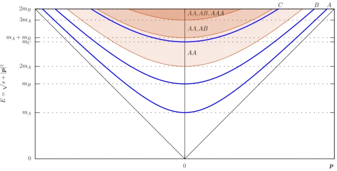
Figure 1.2.1: The low-energy spectrum of a typical theory. The horizontal axis represents the three-dimensional total momentum p. One particle systems are represented in blue.
full space. In other words, in the Hilbert space there is nothing else than particles or com- binations of them (or the absence of them). Hence we vary the labelα= (mi1si1, ...., minsin) and obtain, in addition to the vacuum and to the one-particle states 1,2, ..., N, the so called scattering states, i.e. two-particle states 11,12, ...,1N,22, ..., N N, three-particle states 111,112, ..., N N N and so on, a Fock space.
In Fig. (1.2.1) we can visualise the spectrum in terms of (p, E(p)) of a a typical arbitrary theory which exhibits, within the range shown, three particles with positive masses mA
mB and mC. A central vertical line (0, E(0)≡√
s) represents the energy in the centre of mass. Let’s follow this line from bottom to top, as all other points in the the corresponding hyperboloid are obtained by Eq. (1.2.6). The origin (0,0) represents the vacuum and has zero energy and momentum. The next energy value, which is followed by a mass gap, is obtained at (0, mA) from which all A-particle states can be obtained by Lorentz transformations.
Particle A is the lightest in the theory and all other one-particle states appear at higher energies. The point (0,2mA) represents the threshold of the AA-particle production, i.e.
the starting point of a continuous spectrum of hyperboloids each identified by Eq. (1.2.11) as k increases from zero to infinity. A new threshold AB appears at (0, mA+mB) from which, a new set of continuous states superimposes on that of AA. At even higher energies we have three particle production AAA, the states of the BB system and so on.
Spacetime symmetries are not the only ones we see in our world. The theory can be adapted to include internal symmetries, as isospin, charge conjugation etc., collectively im- plemented by some group G, by enlarging the Hilbert space to be a representation of the direct product groupP ×G. Poincaré and internal symmetries commute so that each can be handled separately. Additional labels will be added to |misi, piσii to identify irreducible states of P ×Gand consequently, additional labels will be added to the tensor product Eq.
(1.2.3) and will be included in ρ and µin Eqs. (1.2.7) and (1.2.8).
The particle states discussed in this section determine a relativistic particle realisation of the abstract in and out states described in Sec. (1.1). We remind the reader that, with the exception of the vacuum and of one-particle states, the specificationin and out is always understood for the particle states - Eqs. (1.2.3),(1.2.7) and (1.2.8) - in order to specify if their labels refer to the infinite past or to the infinite future. Unlike the four-momentum of each particle, the total four-momentum, as well as the total angular momentum, commutes with the Hamiltonian and does not evolve with time. The labelsp j andσj then refer to the eigenvalue of the corresponding operator at any time. The bases Eqs. (1.2.3), (1.2.7) and (1.2.8) are Heisenberg asymptotic states, free10 only at asymptotic times, eigenstates of the Hamiltonian and span the whole (interacting) Hilbert space. In terms of states Eq. (1.2.7), the completeness relation Eqs. (1.1.1) and (1.1.2) reads, for either in orout states,
1=X
a
1 fa
|ai ha|=X
α
Z d4p
(2π)4dΦα|α; p ραi hα; p ρα|. (1.2.15) The sum is over all sets of particlesα, over all total four-momentapand over the whole phase space dΦα. For economy of notation, also the sum over all spin components and internal symmetry indices are understood in R dΦα. The scalar product in H is
hα0; p0ρ0α0|α; p ραi=qNαNα0δαα0(2π)4δ(4)(p−p0)δρ0
α0ρα, (1.2.16) where the normalisationN is a phase space factor that must be compatible with the denom- inator of (1.2.15) oncedΦ, for a givenα, is expressed in terms of the variableρ, symbolically dΦ = dΦdρdρ= N1dρ.
The notion of asymptotic completeness would fail in the presence of bound states: the interaction survives in the infinite future when two particles form a bound state. Asymptotic completeness can be safely retained by simply including all possible bound states in the
10The energies in the tensor products are additive and do not contain an interaction term.
spectrum of the stable one-particle states. We do not question, in this context, whether a stable particle is formed by other particles or not. For instance, in Fig. (1.2.1), particle C may be referred to as a bound state of A and B, but the system, as a whole, is free at asymptotic times. For QCD, the one-particle spectrum includes the pions, protons, the nucleus of the carbon atom, etc. On the contrary, resonances are unstable and do not appear in this spectrum but, as we shall see, have a different origin.
Fields The construction outlined in this section is particle-oriented and does not require the existence of field operators. Indeed, apart from these few lines, no mention of them will be made in this chapter. On the other hand, it is hard to imagine a quantum field theory without fields. If we were to build a Lagrangian (which may be an effective Lagrangian) in terms of some fields defined on Minkowski spacetime and which is capable to represent the physical spectrum, then the quantities that connect the field and particle description are given by the overlaps of general operatorsO(x), built from the fields of the Lagrangian, and the particle states. Examples of these which involve one-particle states are the overlaps of the form h0|O(x)|m s; pσi or more general matrix elements hm s; p0σ0|O(x)|m s; pσi which identify decay constants and form factors, respectively. There does not need to be an operator associated to each one-particle state or vice versa, all that matters are the non-zero overlaps. The operators O(x) can be combined in time-ordered correlation functions and the S-matrix elements, described in detail in the following sections, are obtained from these via the LSZ reduction formula.
1.3 Relativistic scattering
1.3.1 Poincaré invariance of the S -matrix
Except for the vacuum and for one-particle states, the connection between the in and out variants of the particle states is absolutely non trivial and the knowledge of this connection is exactly the aim of scattering theory. The number of independent S-matrix elements can be reduced by the fact that theS matrix commutes withU(a,Λ), or equivalently, theS-matrix is invariant under a Poincaré transformation,
[S, U(a,Λ)] = 0, U(a,Λ)SU−1(a,Λ) =S. (1.3.1)
This implies that, for each generator:
[S, Pµ] = 0, [S, Mµν] = 0. (1.3.2) Therefore, based on our considerations in Sec. (1.1), theSorT matrix elements are diagonal with respect to the total four-momentum and the total angular momentum. Moreover, they are independent ofpandσj. In the three bases Eqs. (1.2.3), (1.2.7) and (1.2.8) we can write hα0; p0i1...p0inσi01...σi0n|T |α; pi1...pimσi1...σimi = (2π)4δ4(p0 −p)T (α0 ←α), (1.3.3) hα0; p0ρ0|T |α; p ρi = (2π)4δ4(p−p0)Tρ[α0ρ0α](s), (1.3.4) hα0; p0j0σj00µ0|T|α; p j σjµi = (2π)4δ4(p−p0)δjj0δσ0
j0σjTµ[α0µ0α]j(s), (1.3.5) where s = p2. The indices [α0α] identify the channel in which the T-matrix elements are taken and will be dropped only when no confusion can arise. The conservation of the total angular momentum is exploited in the last relation which uses the basis Eq. (1.2.8).
It was previously mentioned that indices of internal symmetries were included in ρ and µ. Namely, say that the vectors at the lhs of Eq. (1.3.5) have well defined total isospin I, µ= (I, cI, µ) andµ0 = (I0, c0I, µ0) where cI labels the particular vector in theI subspace and
¯
µ all remaining indices. Then, if isospin is a symmetry of the theory, the Kronecker deltas δII0δcIc0
I can be extracted from the T-matrix element at the rhs, Tµ[α0µ0α]j(s) =δII0δcIc0
ITµ[α0µ0α]jI(s), (1.3.6) resulting in aT-matrix independent of cI and with an explicit label I.
1.3.2 Two particle scattering
Two-particle states were explicitly discussed in Sec. (1.2.2) and we focus now on the scat- tering of these, i.e., we focus on the particular case of Sec. (1.3.1) where AB → CD. The masses and the spins of the i-th particle are denoted by (mi, si) and, in some frame of reference, the four-momenta are
pi = (Ei,pi) with p2i =m2i ⇒ Ei2 =m2i +|pi|2, i=A, B, C, D. (1.3.7)
The process is described by the T-matrix element Eq. (1.3.3) with α= (mAsA, mBsB) and α0 = (mCsC, mDsD). Apart from the spin variables, there are sixteen degrees of freedom for the four-particle system, pi = (Ei,p). Four are constrained by the masses which are fixed and an additional restriction comes from the four-momentum conservation:
pA+pB =pC +pD ⇐⇒
EA+EB =EC +ED pA+pB =pC+pD
Finally, Lorentz invariance adds six further restrictions, so that a 2 → 2 scattering can be described by just two variables. Hence, multiple kinematic situations in terms of pi lead to the same value for theT matrix and only two variables have to be considered. We can choose these variables to be Lorentz invariant, so that the scattering formulae are the same in any frame. In particular, any two of the following Mandelstam variables is a possible choice
s = (pA+pB)2 ≡(pC+pD)2, (1.3.8) t = (pA−pC)2 ≡(pB−pD)2, (1.3.9) u = (pA−pD)2 ≡(pB−pC)2, (1.3.10) as their sum is fixed by
s+t+u=m2A+m2B+m2C +m2D. (1.3.11) The variables, already introduced in Sec. (1.2.2), is the square of the centre-of-mass energy and t is the momentum transfer squared. Then, Eq. (1.3.3) can be written as
hCD; pCpD, σCσD|T|AB; pApB, σAσBi= (2π)4δ(4)(pA+pB−pC −pD)TσCσD,σAσB(s, t). (1.3.12) We have a set of (2sA+ 1) (2sB+ 1)×(2sC + 1) (2sD+ 1) functions. Further symmetries, as parity or time reversal may reduce this number. The physical domain of definition of TσCσD,σAσB(s, t) depends on the masses of the particles. It is clear that
s≥sth= maxn(mA+mB)2,(mC+mD)2o, (1.3.13) wheresthis the threshold for the scattering to occur. The condition ontis more complicated and for general masses it can be found in Ref. [6].
An alternative choice of variables is the absolute value of the relative momentum of the


![Table 3.1: Charmed-strange spectrum up to J P = 2 + . The values are from the PDG [7].](https://thumb-eu.123doks.com/thumbv2/1library_info/3848801.1515297/80.918.254.686.141.300/table-charmed-strange-spectrum-j-p-values-pdg.webp)
![Table 3.2: The six ensembles employed. Details can be found in Ref. [46].](https://thumb-eu.123doks.com/thumbv2/1library_info/3848801.1515297/83.918.98.835.143.298/table-ensembles-employed-details-ref.webp)