Testing for additivity in nonparametric quantile regression

SFB 823

Testing for additivity in nonparametric quantile regression

Discussion Paper

Holger Dette, Matthias Guhlich, Natalie Neumeyer

Nr. 52/2011

Testing for additivity in nonparametric quantile regression

Holger Dette, Matthias Guhlich Ruhr-Universit¨at Bochum

Fakult¨at f¨ur Mathematik 44780 Bochum, Germany

e-mail: holger.dette@rub.de

Natalie Neumeyer Universit¨at Hamburg Fachbereich Mathematik 20146 Hamburg, Germany

e-mail: neumeyer@math.uni-hamburg.de

December 22, 2011

Abstract

In this article we propose a new test for additivity in nonparametric quantile regression with a high dimensional predictor. Asymptotic normality of the corresponding test statistic (after appropriate standardization) is established under the null hypothesis, local and fixed alternatives. We also propose a bootstrap procedure which can be used to improve the approximation of the nominal level for moderate sample sizes. The methodology is also illustrated by means of a small simulation study, and a data example is analyzed.

AMS Subject Classification: 62G05, 62G20

Keywords and Phrases: nonparametric regression, quantile regression, bootstrap, additive estima- tion

1 Introduction

Quantile regression was introduced by Koenker and Bassett (1978) as a complement to least squares estimation (LSE) or maximum likelihood estimation (MLE) and leads to far-reaching ex- tensions of “classical” regression analysis by estimating families of conditional quantile surfaces, which describe the relation between a one-dimensional response y and a high dimensional predic- tor x. Since its introduction it has found great attraction in mathematical and applied statistics because of its ease of interpretation and robustness, which yields attractive applications in such important areas as medicine, economics, engineering and environmental modeling. The interested reader is referred to the recent monograph of Koenker (2005). Many authors consider parametric

quantile regression models but in the last two decades nonparametric methods for estimating con- ditional quantiles have also been discussed intensively. Most of the literature refers to models with a univariate predictor [see e.g. Yu and Jones (1997), Yu and Jones (1998), Dette and Volgushev (2008) and Chernozhukov et al. (2010)]. While from a theoretical point of view there is no difficulty to generalize this methodology to high-dimensional covariates, it is well known that in practical applications such nonparametric methods suffer from the curse of dimensionality and therefore do not yield precise estimates of conditional quantile surfaces for reasonable sample sizes. A common approach in nonparametric statistics to deal with this problem is to postulate an additive non- parametric model, which allows the estimation of the regression with one-dimensional rates. In classical regression (estimating the conditional expectation of the response given in the predictor) this methodology has found considerable interest in the literature [see Linton and Nielsen (1995), Mammen et al. (1999), Carroll et al. (2002), Hengartner and Sperlich (2005), Nielsen and Sperlich (2005), among others]. In quantile regression nonparametric models of this type have only been discussed more recently. Doksum and Koo (2000) suggest a spline estimate and De Gooijer and Zerom (2003) introduce a marginal integration estimate of an additive quantile regression model.

Horowitz and Lee (2005) propose a two step procedure, which fits a parametric model in the first step (with increasing dimension) for each coordinate and smooth it in a second step by the local polynomial technique. Lee et al. (2010) suggest backfitting methods for additive quantile regression estimation, while Dette and Scheder (2011) combine marginal integration techniques with monotone rearrangements [see Dette et al. (2006)] for the construction of additive estimates.

Although these methods estimate the unknown quantile regression with the optimal (one-dimensional) rate if the assumption of an additive model is correct, they are generally inconsistent if the quan- tile regression is not additive. In this case the corresponding statistics usually estimate a “best approximation” of the unknown regression by an additive quantile regression model, but the dif- ference between the “true” curve and its best approximation can be substantial. For this reason, it is of some importance to investigate by a statistical test if the hypothesis of an additive quantile regression is satisfied. In the context of modeling the conditional expectation this problem has found considerable interest in the literature [see for example Eubank et al. (1995), Gozalo and Linton (2001), Dette and von Lieres und Wilkau (2001), Derbort et al. (2002) or Abramovich et al. (2009), among others]. On the other hand, to the best knowledge of the authors, tests for the hypothesis of an additive quantile regression model have not been considered so far in the literature, and the purpose of the present paper is to propose and analyze such a procedure for this problem. In Section 2 we introduce the basic notation and an additive estimate of the conditional quantile curve. The test statistic for the problem of additive quantile regression uses the residuals from this additive fit and is introduced in Section 3, where we also study the main asymptotic properties. In particular, we prove weak convergence of an appropriately standardized version of the test statistic under the null hypothesis and fixed alternatives with different rates corresponding to both cases. In Section 4 we present a small simulation study in order to illustrate the finite sample properties of a bootstrap version of the proposed test. We also investigate a data

example testing if the hypothesis of an additive quantile regression is satisfied. Finally, all proofs and some of the more technical details in the proofs are deferred to an appendix in Section 5, 6 and 7.

2 Preliminaries - an additive estimator

Consider a sequence of independent identically distributed observations (X₁, Y₁), . . . ,(X_n, Y_n) where X_j = (X_j1, . . . , X_jd)^T denotes a d−dimensional random variable with density f and f_i is the marginal density of the ith component X_ji of X_j (i= 1, . . . , d). Throughout this paper we denote by F(y|x) the conditional distribution function of Y1 givenX1 =x= (x1, . . . , xd)^T and by Q(τ|x) =F⁻¹(y|x) the corresponding conditional quantile function. In the following we fix some τ ∈(0,1) and are interested in the problem of testing the hypothesis of additivity

(2.1) H₀ :Q(τ|x) =Q(τ|x₁, . . . , x_d) =

d

X

k=1

Q_k(τ|x_k) +c(τ)

for some constant c(τ) and functions Q_k(τ|x_k) (k = 1, . . . , d). Note that the quantities in (2.1) are not uniquely determined and in order to make these identifiable we assume throughout this paper the conditions

E[Q_k(τ|X_jk)] = 0, k= 1, . . . , d, j = 1, . . . , n.

For the construction of a test for the hypothesis (2.1) let ˆQ_add denote an additive estimate of the quantile regression function Q(for fixedτ), which will be specified later. We propose the statistic

(2.2) T_n= 1

n(n−1)

n

X

i=1 n

X

j6=i

L_g(X_i−X_j)Rb_iRb_j,

where the random variables Rb_i are defined by

(2.3) Rb_i =I{Y_i ≤Qb⁻ⁱ_add(τ|X_i)} −τ,

the functionLdenotes ad-dimensional kernel function with bandwidthg and here and throughout this paper we use the notation

L_g(X_i−X_j) = 1

g^dLX_i −X_j g

. (2.4)

Throughout this paper we use the notation ba and ba⁻ⁱ corresponding to estimates from the full sample{(X_j, Y_j)|j = 1, . . . , n}and the sample without theith observation, respectively. Thus the statisticQb⁻ⁱ_add(τ|x) in (2.3) denotes the additive (nonparametric) estimate of the quantile regression from the sample without theith observation. Similarly,Qb^−i,j_add andQb^−i,j,k_add denote the corresponding

estimators without theith andjth and the ith,jth andkth observation, respectively. Various ad- ditive quantile regression estimates have been proposed by De Gooijer and Zerom (2003), Horowitz and Lee (2005), Lee et al. (2010) and Dette and Scheder (2011).

Note that statistics of the type (2.4) have been introduced by Zheng (1996) in the context of testing for a specific parametric form in nonparametric regression, and since its introduction has found considerable interest in the context of goodness-of-fit tests [see Dette and von Lieres und Wilkau (2001) or Zhang and Dette (2004) among others]. In the following section we will study the asymptotic properties of the test statistic under the null hypothesis of additivity, local alternatives and fixed alternatives. In particular, we prove weak convergence of a standardized version of the statistic T_n defined in (2.2) with different rates corresponding to the null hypothesis and fixed alternatives. For this discussion which is deferred to Section 3 we therefore recall the definition of an additive quantile regression estimate which has recently been introduced by Dette and Scheder (2010) and will be used throughout this paper for a test of an additive quantile regression. Let F(·|x) denote the conditional distribution function of Y_j, given X_j = x. Following Dette and Scheder (2011) we denote by

(2.5) Fbl(y|x) = Pn

i=1K_1,h1(x_l−X_il)K_2,H(x_l−X_il)I{Y_i ≤y}

Pn

i=1K_1,h1(x_l−X_il)K_2,H(x_l−X_il)

the Nadaraya Watson estimate of the conditional distribution function where for l = 1, . . . , d, x_l ∈ R^d−1 denotes the vector containing the components x₁, . . . , xl−1, x_l+1, . . . , x_d of the vector x = (x₁, . . . , x_d)^T ∈ R^d. In (2.5) the functions K₁ and K₂ are one-dimensional and (d− 1)- dimensional kernels, respectively, h₁ is a one-dimensional bandwidth and H = diag(h₂, . . . , h_d) a (d−1)-dimensional non-singular and diagonal (bandwidth) matrix and we use the notation

K1,h1(x1) = K1(x1/h1)h1, K_2,H(˜x) = 1

det(H)K₂(H⁻¹x).˜

We also note that the statistics Fb_l differ only by the component of the predictor, which is used in the kernel K₁ but not in K₂ and that (under appropriate assumptions) all of them estimate the conditional distribution function consistently. Moreover, for different values of l = 1, . . . , d different bandwidths h₁ =h_1,l, h₂ =h_2,l will be used in the estimate Fb_l, although this will not be reflected in our notation. Throughout this paper we denote by G:R→[0,1] a strictly increasing given distribution function, which can be specified by the data analyst and denote byK a further positive one-dimensional kernel with compact support, say [−1,1] with corresponding bandwidth b_n. Following Dette and Volgushev (2008) we define

(2.6) Qb_l,N(τ|x) =G⁻¹(Gb_l,N(τ|x)), where the statistic Gbl,N is given by

(2.7) Gb_l,N(τ|x) = 1 N

N

X

i=1

Z τ

−∞

K_bn Fb_l

G⁻¹ i N

x

−u du

and we use the notation Kbn(x) = K(x/bn)/bn. Note that intuitively (for example if Fbl(y|x) is uniformly consistent) we obtain for N → ∞, n→ ∞,b_n→0 the approximation

Gb_l,N(τ|x)≈G_N(τ|x) := 1 N

N

X

i=1

Z τ

−∞

K_bn F

G⁻¹ i N

x

−u du (2.8)

≈ Z

I{F(G⁻¹(s)|x)≤τ}ds =G(Q(τ|x)),

and therefore the statistic Qb_l,N(τ|x) defined in (2.6) is a reasonable estimate of the conditional quantile curveQ(τ|x) = F⁻¹(τ|x). Dette and Volgushev (2008) demonstrate that the choice of the distribution function G has a negligible impact on the quality of the resulting estimate provided that an obvious centering and standardization is performed. Similarly, the estimate ˆQ_l,N(τ|x) is robust with respect to the choice of the bandwidth b_n if it is chosen sufficiently small [see Dette et al. (2006)]. The estimate (2.6) suffers from the curse of dimensionality if the dimension d of the predictor is large and for this reason Dette and Scheder (2011) propose to combine it with the marginal integration technique in order to obtain an additive estimate of the quantile regression with a one-dimensional rate of convergence. To be precise define

qbl(τ|xl) = 1 n

n

X

j=1

Qbl,N(τ|xl, Xjl), l= 1, . . . , d as an estimate of the first marginal effect

q_l(τ|x_l) :=

Z

Q(τ|x)f_l(x_l)dx_l =Q_l(τ|x_l) +c(τ), (2.9)

wheref_l :R^d−1 →Ris the density of the random vector (X_j1, . . . , X_jl−1, X_jl+1, . . . , X_jd)^T and the second equality in (2.9) holds under H₀. The estimates of the marginal effects qb_l(τ|x_l) are now used to define the final additive estimate of the conditional quantile function which is given by (2.10) Qbadd(τ|x) :=

d

X

k=1

bqk(τ|xk)− 1− 1

d X^d

k=1

1 n

n

X

i=1

bqk(τ|Xik).

We note that this statistic is well defined even in the case when the null hypothesis (2.1) is not satisfied and in this case it estimates consistently (under appropriate assumptions) the function

Q_add(τ|x) =

d

X

j=1

Q_j(τ|x) +c(τ),

where the quantities Qj are defined as in (2.9). Throughout this paper we make the following assumptions regarding the kernels used in the definition of (2.2), (2.5) and (2.7).

Assumption 2.1. The one-dimensional kernel K1 in (2.5) is of bounded variation and has com- pact support [−1,1] with existing moments of order 2 satisfying

Z 1

−1

xK1(x)dx= 0, c₂(K₁) = 1

2 Z 1

−1

x²K₁(x)dx.

Similarly for a multi index ν₁ = (ν₂, . . . , ν_d) ∈ N^d−1 we define the monomial x^ν₁¹ = x^ν₂², . . . x^ν_d^d, denote by |v₁|:=Pd

i=2ν_i the corresponding degree.

Assumption 2.2. We assume that the kernel K₂ in (2.5) is a (d−1)-dimensional kernel of order q with support [−1,1]^d−1, that is

(i) K₂ is symmetric, (ii)

Z

[−1,1]^d−1

K2(x1)dx1 = 1, (iii)

Z

[−1,1]^d−1

|x^ν₁¹||K₂(x₁)|dx₁ <∞ for |ν₁| ≤q, (iv)

Z

[−1,1]^d−1

x^ν₁¹K₂(x₁)dx₁ = 0 for 1≤ |ν₁| ≤q−1, (v)

Z

[−1,1]^d−1

x^ν₁¹K₂(x₁)dx₁ 6= 0 for some |ν₁|=q,

and is of bounded variation.

The one-dimensional kernel K and thed-dimensional kernel Lsatisfy Assumption 2.3.

The kernel K is Lipschitz continuous with compact support [−1,1].

The kernel L is a d-dimensional symmetric kernel of order 2 with compact support [−1,1]^d and satisfies L(x)<∞, L(x)≥0 for all x∈[−1,1]^d

3 Asymptotic theory

In this section we study the asymptotic properties of the statistic introduced in Section 2 for testing the hypothesis of an additive quantile regression. We begin with a statement regarding weak convergence under the null hypothesis. In order to keep the notation simple we assume that the (d−1)-dimensional bandwidth matrix in the definition of the estimate (2.5) is proportional

to the identity matrix, that is H = diag(h2, . . . , h2)∈R(d−1)×(d−1)

, where h2 is a one dimensional bandwidth. We also introduce the notation K_2,h2(x) instead of K_2,H(x) in this case. Moreover, in order to present a result regarding weak convergence under the null hypothesis we make the following basic assumptions.

Assumption 3.1.

1. The random variables X_j have a positive density f ∈ C^q([0,1]^d) with support supp(f) = [0,1]^d, where q ≥ d and C^q([0,1]^d) denotes the set of all q times continuously differentiable functions defined on the unit cube [0,1]^d.

2. For any x the functionF(·|x) is strictly increasing and continuously differentiable with uni- formly bounded derivative.

3. The distribution functionGis twice continously differentiable and(G⁻¹)⁰ is uniformly bounded on closed intervals I ⊂(0,1).

4. For any x the function Q(·|x) is twice continuously differentiable in a neighbourhood of τ and there exists ε >0 such that

sup

x∈[0,1]^d

sup

|s−τ|<ε

Q⁰(s|x)<∞, sup

x∈[0,1]^d

sup

|s−τ|<ε

Q⁰⁰(s|x)<∞.

5. For each l= 1, . . . , d, the bandwidths g, b_n, h₁, h₂ used in the estimate Fb_l in (2.5) satisfy the following conditions (if n → ∞)

N =O(n), b_n =o(h₁) g^d=o(h²₁), nh⁵₁ =O(1)

ng^d → ∞, nb_n→ ∞, nh₁h^d−1₂ → ∞ h^q₂ =o(h²₁), nh^2q+1₂ =O(1)

Assumption 3.2.

For each l= 1, . . . , d, the bandwidths g, b_n, h₁, h₂ used in the estimate Fb_l in (2.5) satisfy the following conditions (if n → ∞)

n^2α

nh₁h^d−1₂ b²_n =o(1) n^2αg^d2 1

h1h^d−1₂ =o(1) for some α >0.

The following result establishes weak convergence of the test statisticTndefined in (2.2) . Through- out this paper the symbol −→^D denotes weak convergence.

Theorem 3.3. If Assumption 2.1, 2.2, 2.3, 3.1, 3.2 and the null hypothesis (2.1) of an additive quantile regression model are satisfied, it follows that

(3.1) ng^d/2T_n −→ N^D (0, σ²),

where the asymptotic variance is given by

(3.2) σ² = 2τ²(1−τ)²

Z

L²(u)du Z

f²(x)dx.

Remark 3.4. We would like to point out that a result of the form (3.1) is typical for the limit distribution of a statistic of the type defined in (2.2) [see Gozalo and Linton (2001), or Dette and von Lieres und Wilkau (2001)]. For example, recently H¨ardle et al. (2012) considered the problem of testing the hypothesis of causality in quantile regression, which reduces in the simplest case to the hypothesis (for a given l ∈ {1, . . . , d})

H₀^c:Q(τ |x) = Q(τ |xl).

This hypothesis means that the conditional quantile given X = x does not depend on the com- ponents x₁, . . . , xl−1, x_l+1, . . . , x_d of the vector x. H¨ardle et al. (2012) proposed a statistic of the form (2.2), where the residuals ˆR_i are replaced by ˜R_i =I{Y_i ≤Q(τ|Xˆ _il)}and ˆQ(τ|x_l) is an appro- priate estimate of the conditional quantile function under the null hypothesis H₀^c. They claimed asymptotic normality of a normalized test statistic

J_n= 1 n(n−1)

X

i6=j

L_g(X_i−X_j) ˜R_iR˜_j

with the same limit distribution as given in Theorem 3.2. However, it should be pointed out here that the proof in this paper is not correct. The basic argument of H¨ardle et al. (2012) consists in the statement that the fact

sup

x

|Q(τ|xˆ _l)−Q(τ|x_l)|≤C_n results in the estimate

(3.3) J_nU ≤J_n ≤J_nL

where the statistics J_nU and J_nL are defined by JnU = 1

n(n−1) X

i6=j

Lg(Xi−Xj)εiUεjU,

J_nL = 1 n(n−1)

X

i6=j

L_g(X_i−X_j)ε_iLε_jL,

and ε_iU = I{Y_i +C_n ≤ Q(τ|X_il)} −τ, ε_iL =I{Y_i+C_n ≤ Q(τ|X_il)} −τ (see equation (A.11-3) in this paper). A simple calculation shows that this conclusion is not correct and in fact the inequality (3.3) does not hold in general. It turns out that the proof of Theorem 1 in H¨ardle et al.

(2012) can not be corrected easily.

However, using similar arguments as given in the proof of Theorem 3.2, it can be shown that a similar statement of weak convergence holds for a slightly modified statistic considered in H¨ardle et al. (2012), that is

g^d/2 (n−1)

X

i6=j

L_g(X_i−X_j)(I{Y_i ≤Qˆ⁻ⁱ(τ|X_il)} −τ)(I{Y_j ≤Qˆ^−j(τ|X_jl)} −τ)−→ N^D (0, σ²)

where ˆQ⁻ⁱ(τ|X_il) denotes the quantile regression estimate of Dette and Volgushev (2008) frome the two-dimensional sampe (X_il, Y_i)ⁿ_i=1 andσ² is defined in (3.2) (we omit details here for the sake of brevity). A correct proof of the result claimed in H¨ardle et al. (2012) is still an open problem.

In the following discussion we investigate the asymptotic properties of the statistic T_n defined in (2.2) under local and fixed alternatives. For this purpose we introduce the “residuals”

(3.4) Rj =I{Yj ≤Q(τ|Xj)} −τ

and denote by

(3.5) ∆(X_j) =E[R_j −R^add_j |X_j] =−E[R^add_j |X_j]

the conditional expectation of the distance between the “residuals” defined before and the “re- stricted residuals”

(3.6) R^add_j =I{Y_j ≤Q_add(τ|X_j)} −τ

obtained from the best additive approximation. Note that under the null hypothesis we have

∆(Xj) = 0 a.s., while under the alternative it follows that P(∆(Xj) = 0) < 1. We first consider the properties of the test for local alternatives of the form

(3.7) Q(τ|x) =Q_add(τ|x) +d_nl(x),

where d_n denotes a sequence satisfying d_n= (ng^d/2)^−1/2 →0 as n→ ∞ and the function l(·) and its first-order derivatives are bounded.

Theorem 3.5. Assume that Assumption 2.1, 2.2, 2.3, 3.1 and 3.2 are satisfied. Under local alternatives of the form (3.7) with d_n= 1/(n^1/2g^d4) it follows that

(3.8) ng^d2T_n −→ N^D (µ, σ²),

where the asymptotic variance and bias are given by (3.2) and µ=E[(F⁰(Q(τ|X₁)|X₁))²l²(X₁)f(X₁)], respectively.

The following result specifies the asymptotic distribution of the test statistic T_n defined in (2.2) under fixed alternatives. For its proof we require the following additional assumptions

Assumption 3.6.

1. For any y ∈R we have F(y|·)∈C_b^q([0,1]^d).

2. We assume the representation

I{Y_j ≤y} −F(y|X_j) =s(y|X_j)ε_j, j = 1, . . . , n, (3.9)

where s²(y|x) = F(y|x)(1−F(y|x)) and the ε_j are independent of Y_j, but may depend on X_j. We moreover assume that sup_xE[ε⁴_j|X_j =x]<∞.

3. For each l= 1, . . . , d, the bandwidths g, b_n, h₁, h₂ used in the estimate Fb_l in (2.5) satisfy the following conditions (if n → ∞)

logn

nh²₁h^2(d−1)₂ b²_n =o(1) n^2α−1/2

h₁h^d−1₂ =o(1), for some α >0

Note that in model (3.9) the random variables are independent identically distributed with with E[ε_j|X_j] = 0, Var(ε_j|X_j) = 1. Moreover this model is a common assumption in quantile regression [see Hall et al. (1999) or Dette and Scheder (2011) among others] and observing (3.4) we have (3.10) s(Q(τ|X_j)|X_j)ε_j =I{Y_j ≤Q(τ|X_j)} −τ =R_j.

Theorem 3.7. If Assumption 2.1, 2.2, 2.3, 3.1 and 3.6 are satisfied and the null hypothesis (2.8) does not hold, then we have as n→ ∞

(3.11) n^1/2(T_n−E[T_n])−→ N^D (0, σ²),

where

E[T_n] = E[∆²(X₁)f(X₁)] + 2Eh

F⁰(Q_add(τ|X₁)|X₁)∆(X₁)f(X₁)

b(X₁)− 1− 1

d

b(X₂)i h²₁ +o(h²₁) +O(g²)

with b(x) = Pd

α=1b_α(x_α) and b_α(x_α) = c₂(K₁)

Z 1 2

∂²

∂x²_αF(Q(τ|x_α, t_α)|x_α, t_α) F⁰(Q(τ|x_α, t_α)|x_α, t_α) (3.12)

+

∂

∂xαF(Q(τ|x_α, t_α)|x_α, t_α)_∂x^∂

αf(x_α, t_α) F⁰(Q(τ|x_α, t_α)|x_α, t_α)f(x_α, t_α)

f_α(t_α)dt_α. The asymptotic variance in (3.11) is given by

σ² = 4Varh

∆²(X₁)f(X₁)−E

∆(X₂)f(X₂)F⁰(Q_add(τ|X₂)|X₂)X^d

α=1

Q(τ|X_2α, X_1α)

− 1− 1

d X^d

α=1

Q(τ|X_1α, X_3α) +Q(τ|X_3α, X_1α) X₁i + 4τ(1−τ)Eh

∆(X₁)f(X₁) +

d

X

α=1

f_α(X_1α)

f(X1)F⁰(Q(τ|X1)|X1) Z

∆(X_1α, t_α)f²(X_1α, t_α)F⁰(Q_add(τ|X_1α, t_α)|X_1α, t_α)dt_α

−(d−1) 1

F⁰(Q(τ|X₁)|X₁) Z

∆(t)f²(t)F⁰(Q_add(τ|t)|t)dt2i .

Remark 3.8. Note that Theorem 3.3 provides an asymptotic levelα test for the hypothesis (2.1) of an additive quantile regression model by rejecting H₀, whenever

T_n>σˆ_nu1−α,

where ˆσ²_n is an appropriate estimate of the asymptotic variance σ² defined in (3.2). Moreover, by Theorem 3.7 it follows that this test is consistent, because under the alternative we have

T_n −→^D E[∆²(X₁)f(X₁)]>0 from this result.

4 Finite sample properties and a data example

4.1 A small simulation study

In order to investigate the finite sample properties of the nwe test we have performed a small simulation study. To be precise, we consider the median regression model

Y_i =Q(0.5|X_i) + 0.25ε_i

where εi are independent, standard normally distributed and independent of the bivariate covari- ates X_i = (X_i1, X_i2), i= 1, . . . , n. For the choice of the predictor we investigate the following two scenarios.

(A) X_i are uniformly distributed on the unit square [0,1]²

X_i = (X_i1, X_i2)∼ U([0,1]²), i= 1, . . . , n (B) X_i = (X_i1, X_i2) are given by

X_i1 = 1 2 + 1

π arctan(Z_i1) X_i2 = 1

2 + 1

π arctan(Z_i2)

whereZ_i = (Z_i1, Z_i2) are (independent) centered normally distributed random variables with variance 1 and correlation ρ= 0.2, ρ= 0.5, ρ= 0.8.

Note that in Design A the random variables X_i1 and X_i2 are independent, whereas Design B represents a situation whereX_i1 andX_i2 are correlated. In our simulation study we consider three models for the conditional quantile function, that is

Q(0.5|x₁, x₂) =x₁+x₂ (4.1)

Q(0.5|x₁, x₂) =x²₁+x²₂ (4.2)

Q(0.5|x₁, x₂) = cos(cπ(x₁+x₂)), c= 0.5,1,2, (4.3)

where the first two cases correspond to the null hypothesis of additivity and (4.3) represents three alternatives. For all kernels in our estimators we use the Epanechnikov kernel K(t) =

3

4(1−t²)I_[−1,1](t), and a product of two kernels of this type as a two-dimensional kernel. Following Dette and Scheder (2011) the bandwidths are chosen as

h1 = 0.6n⁻¹⁵, h2 = 0.2n⁻¹⁵, bn= 0.1n⁻¹⁴, g= 0.1n⁻¹⁴.

In similar problems it has been observed by several authors [see Fan and Linton (2003)] that the asymptotic normal distribution under the null hypothesis does not provide a satisfactory approximation for the distribution of the statistic T_n for small sample sizes. For this reason many authors propose the application of a bootstrap in this context to calculate critical values. We follow this suggestion and use a wild bootstrap for this purpose. To be precise, in the τ-quantile model we define a bootstrap sample by

Y_i^∗ = ˆQ_add(τ|X_i) +v_i|Y_i−Qˆ_N(τ|X_i)|,

where Qb_add and Qb_N are defined in Section 2 and v_i denote independent identically distributed random variables satisfying P(v_i = −1) = τ and P(v_i = 1) = 1 −τ, which are independent

from the original sample. A similar bootstrap data generation was suggested by Sun (2006) The bootstrap observations, conditionally on the original sample, fulfill H₀ and additionally fulfill a τ-quantile regression model because

P^∗(Y_i^∗ ≤Qˆ_add(τ|X_i)|X_i =x) = P(v_i ≤0) =τ,

where P^∗ denotes the probability conditionally on (X_j, Y_j), j = 1, . . . , n. Note also that for the median model used in the simulations we have τ = ¹₂ and v_i are Rademacher variables. The critical value for the test is then obtained from the bootstrap distribution

P^∗(T_n^∗ ≥t^∗_n,(1−α)) = 1−α,

and the hypothesis of additivity is rejected ifTn ≥t^∗_n,(1−α). For the estimation oft^∗_n,(1−α) we choose the number of bootstrap replications asB = 100 and we have simulated the rejection probabilities of this test on the basis of 1000 replications of each experiment.

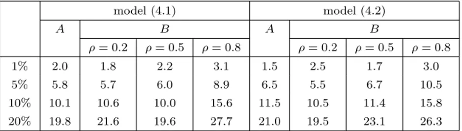
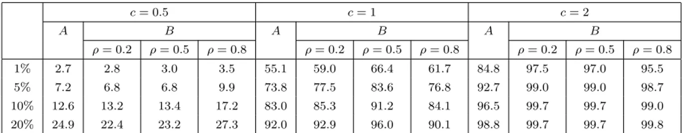
In Table 1 we display the results of the simulation study for model (4.1) and (4.2) forn = 100 which represent the null hypothesis. The corresponding results under the alternative defined by model (4.3) are shown in Table 2. Under the null hypothesis we observe a reasonable approximation of the nominal level under Design A and B provided that the correlation between the explanatory variables in the latter case is not too large [see Table 1]. If ρ= 0.8 in Design B the nominal level is overestimated, which means that the critical values of the bootstrap procedure are too small.

The results in Table 2 demonstrate that the bootstrap test detects alternatives with reasonable power in all cases under investigation.

model (4.1) model (4.2)

A B A B

ρ= 0.2 ρ= 0.5 ρ= 0.8 ρ= 0.2 ρ= 0.5 ρ= 0.8

1% 2.0 1.8 2.2 3.1 1.5 2.5 1.7 3.0

5% 5.8 5.7 6.0 8.9 6.5 5.5 6.7 10.5

10% 10.1 10.6 10.0 15.6 11.5 10.5 11.4 15.8

20% 19.8 21.6 19.6 27.7 21.0 19.5 23.1 26.3

Table 1: Simulated level of the bootstrap test for the hypothesis of an additive quantile regression model under the null hypothesis of additivity.

4.2 A data example

Recently Dette and Scheder (2011) applied additive quantile regression to investigate the Boston housing data, which has been analyzed by several authors. The dataset contains the housing values of suburbs of Boston and 13 variables, which might have an influence on the housing prices like pollution, crime and urban amenities. This dataset has been analyzed by several authors, also in the context of quantile regression. Dette and Scheder (2011) focus on the four covariates