Automatic Stabilization and Redistribution in Europe and the US
Inauguraldissertation zur
Erlangung des Doktorgrades der
Wirtschafts- und Sozialwissenschaftlichen Fakultät der
Universität zu Köln
2012 vorgelegt
von
Dipl.-Volksw. Mathias Dolls
aus Herford (Nordrhein-Westfalen)
Korreferent: Prof. Dr. Felix Bierbrauer Tag der Promotion: 28. August 2012
Acknowledgements
This book contains work that was written when I was a doctoral fellow at the Cologne Graduate School in Management, Economics and Social Sciences (CGS) at the University of Cologne, a Research A¢ liate and later a Research Associate at the Institute for the Study of Labor (IZA). I am grateful for the scholarship I received from CGS which included …nancial support from the State of North Rhine Westfalia and the University of Cologne. I have appreciated the supportive and friendly working environment at CGS and IZA and I wish to thank my colleagues at both places for many stimulating discussions.
I am grateful to Clemens Fuest for supervising my dissertation though becoming Research Director of the Oxford University Centre for Business Taxation in 2008.
He is also coauthor of the essays in chapters 2 and 3 in this book. I also wish to thank Felix Bierbrauer who became Professor for the Chair in Public Economics at the University of Cologne in 2011 and who kindly agreed to be the second supervisor of this thesis.
I am deeply indebted to Andreas Peichl for the motivating and inspiring col- laboration throughout my time as a doctoral student. He is coauthoring the essays in chapters 2-4. Special thanks go to the other coauthors of the essay in chapter 4, Olivier Bargain, Herwig Immervoll, Dirk Neumann, Nico Pestel and Sebastian Siegloch. It has always been a great pleasure to work with them on this and other joint research projects. I would like to thank Daniel Feenberg for granting me access to NBER’s TAXSIM model and helping me with the simulations and nu- merous other people at workshops and conferences for their valuable comments.
Last but not least, I would like to express my gratitude to my wife and my family for all their encouragement and support.
List of Figures iii
List of Tables v
1 Introduction 1
1.1 Motivation and key questions . . . 1
1.2 Empirical approach: Counterfactual simulations . . . 4
1.3 Summary of results . . . 6
2 Automatic stabilizers and economic crisis: US vs. Europe 9 2.1 Introduction . . . 9
2.2 Previous research and theoretical framework . . . 13
2.2.1 Previous research . . . 13
2.2.2 Theoretical framework . . . 16
2.3 Data and methodology . . . 22
2.3.1 Microsimulation using TAXSIM and EUROMOD . . . 22
2.3.2 Scenarios . . . 23
2.4 Results . . . 24
2.4.1 US vs. Europe . . . 24
2.4.2 Country decomposition . . . 26
2.4.3 Demand stabilization . . . 28
2.4.4 Extensions: Employer social insurance contributions, con- sumption taxes and in-kind bene…ts . . . 31
2.5 Discussion of the results . . . 35
2.5.1 Stabilization coe¢ cients and macro estimates . . . 35 i
ii CONTENTS
2.5.2 Automatic stabilizers and openness . . . 38
2.5.3 Automatic stabilizers and discretionary …scal policy . . . 40
2.6 Conclusions . . . 41
2.7 Appendix . . . 45
2.7.1 Additional results . . . 45
2.7.2 Reweighting procedure for increasing unemployment . . . 55
3 Automatic stabilizers, economic crisis and income distribution in Europe 57 3.1 Introduction . . . 57
3.2 Tax and transfer systems in Europe . . . 60
3.2.1 Tax bene…t systems . . . 60
3.2.2 Distribution and Redistribution . . . 63
3.3 E¤ects of shocks on income distribution . . . 64
3.3.1 Overall distribution . . . 64
3.3.2 Stabilization of di¤erent income groups . . . 67
3.3.3 Income stabilization and redistribution . . . 69
3.3.4 Cluster Analysis . . . 72
3.4 Conclusions . . . 75
3.5 Appendix . . . 77
4 Tax policy and income inequality in the US, 1978-2009: A decom- position approach 80 4.1 Introduction . . . 80
4.2 Literature . . . 83
4.3 Methodology . . . 86
4.3.1 Decomposition . . . 86
4.3.2 Data . . . 90
4.3.3 Sample selection, income concepts and the calculation of counterfactual scenarios . . . 91
4.3.4 Tax history . . . 92
4.4 Results . . . 94
4.4.1 Trends in average tax rates and income inequality . . . 94
4.4.2 Decomposition results . . . 96
4.4.3 Robustness checks . . . 103
4.5 Conclusion . . . 106
4.6 Appendix . . . 108
5 Stabilization, redistribution and the political cycle in the US 126 5.1 Introduction . . . 126
5.2 Automatic Stabilizers in the US, 1978-2010 . . . 128
5.2.1 Overall stabilization . . . 128
5.2.2 State decomposition . . . 129
5.3 Literature . . . 130
5.4 Data and methodology . . . 133
5.4.1 Empirical model . . . 133
5.4.2 Data . . . 134
5.5 Partisan e¤ects . . . 135
5.5.1 Tax burden and income insurance . . . 135
5.5.2 Inequality . . . 139
5.6 Conclusions . . . 142
5.7 Appendix: . . . 144
5.7.1 Results . . . 144
5.7.2 Data appendix . . . 153
6 Concluding remarks 154
Bibliography 158
Curriculum Vitae 173
List of Figures
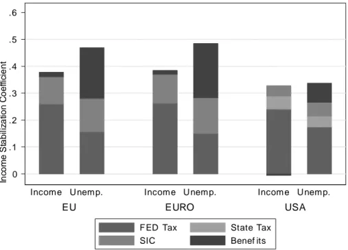
2.4.1 Decomposition of stabilization coe¢ cient for both scenarios . . . 25
2.4.2 Decomposition of income stabilization coe¢ cient in both scenarios for di¤erent countries . . . 27
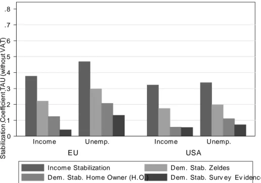
2.4.3 Income vs. demand stabilization . . . 30
2.5.1 Government size and stabilization coe¢ cients . . . 37
2.5.2 Income stabilization coe¢ cient and openness of the economy . . . . 39
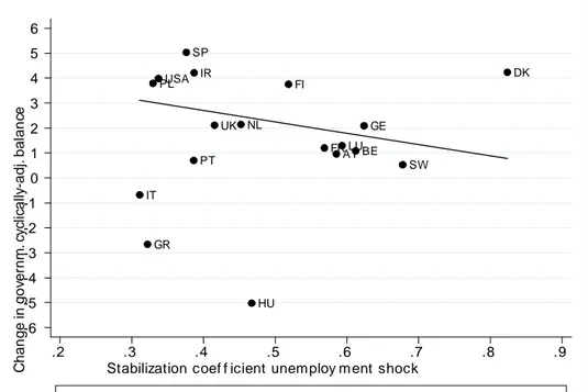
2.5.3 Discretionary measures and income stabilization coe¢ cient . . . 40
2.7.1 Income stabilization incl. in-kind bene…ts . . . 52
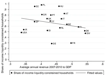
2.7.2 Income share of liquidity constrained households and government revenue . . . 52
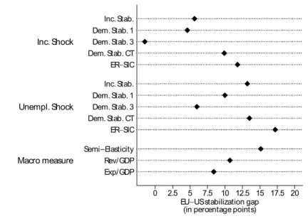
2.7.3 EU-US stabilization gap . . . 53
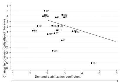
2.7.4 Discretionary measures and demand stabilization . . . 54
2.7.5 Discretionary measures and openness of the economy . . . 54
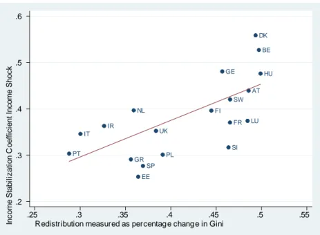
3.3.1 Income Stabilization IS and Redistribution . . . 71
3.3.2 Income Stabilization IS and Ratio Direct to Indirect Taxes . . . 72
3.3.3 Cluster Analysis . . . 74
3.5.1 Income Stabilization US and Redistribution . . . 77
4.6.1 Average tax rates 1978-2009 . . . 118
4.6.2 Trends in market income . . . 119
4.6.3 Income inequality 1978-2009 . . . 119
4.6.4 Absolute inequality and redistribution trends - 90/10 . . . 120
4.6.5 Absolute inequality and redistribution trends - 90/10 - Imputation of itemized deductions. 1978–2006 . . . 120
iv
4.6.6 Absolute inequality and redistribution trends - 90/50 . . . 121
4.6.7 Absolute inequality and redistribution trends - 50/10 . . . 121
4.6.8 Absolute inequality and redistribution trends - Gini . . . 122
4.6.9 Policy e¤ect on average tax rates . . . 122
4.6.10Shapley-value policy and other e¤ects 90/10 . . . 123
4.6.11Shapley-value policy and other e¤ects 90/50 . . . 124
4.6.12Shapley-value policy and other e¤ects 50/10 . . . 124
4.6.13Shapley-value policy and other e¤ects Gini . . . 125
4.6.14Shapley-value policy e¤ect . . . 125
5.7.1 Income stabilization coe¢ cient, 1978-2010 . . . 144
List of Tables
2.4.1 Demand stabilization coe¢ cients . . . 29
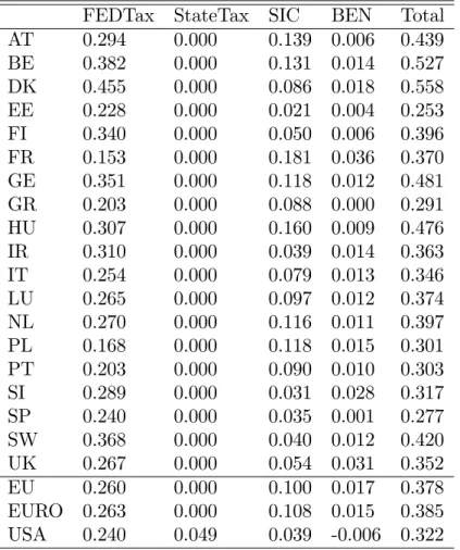
2.7.1 Decomposition income stabilization coe¢ cient for income shock . . 45
2.7.2 Decomposition income stabilization coe¢ cient for unemployment shock . . . 46
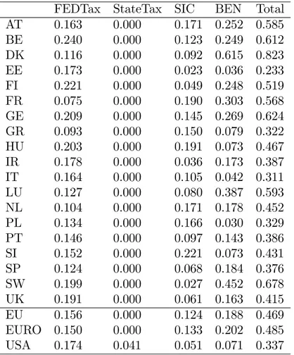
2.7.3 Shares of liquidity constrained households . . . 47
2.7.4 Decomposition income stabilization coe¢ cient including employer SIC . . . 48
2.7.5 Demand stabilization coe¢ cient including consumption taxes . . . . 49
2.7.6 Decomposition of income stabilization coe¢ cient for the income shock into tax bene…t system (column) and population character- istics (row) . . . 50
2.7.7 Correlation between micro and macro estimates . . . 51
3.2.1 Income tax systems 2007 . . . 61
3.2.2 Tax bene…t mix (as % of GDP) in 2005 . . . 62
3.2.3 Distribution and redistribution in the baseline . . . 64
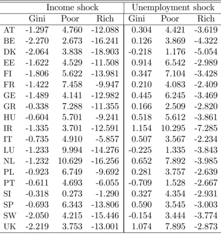
3.3.1 E¤ect of shocks on income distribution . . . 66
3.3.2 Change in distribution and redistribution . . . 67
3.3.3 Stabilization of income groups - Proportional Income Shock . . . . 69
3.3.4 Stabilization of income groups - Unemployment Shock . . . 70
3.3.5 Regressions on income stabilization coe¢ cient IS . . . 73
3.5.1 Stabilization of income groups by components - Income Shock . . . 78
3.5.2 Stabilization of income groups by components - Unemployment Shock 79 4.6.1 Tax Legislation . . . 108
vi
4.6.2 Decomposing changes in income distribution over time . . . 115
4.6.3 Decomposing changes in income distribution over time (cont.) . . . 116
4.6.4 Decomposing changes in income distribution over time (cont.) . . . 117
5.7.1 Income stabilization by component and state, 1978-2010 . . . 145
5.7.2 Income stabilization by component and state, 1978-2010 (cont.) . . 146
5.7.3 Descriptive statistics, 1978-2008 . . . 147
5.7.4 OLS estimation . . . 148
5.7.5 Summary statistics from …rst-stage regression . . . 149
5.7.6 2SLS estimation . . . 150
5.7.7 Choice of time interval . . . 151
5.7.8 Partisan e¤ect on inequality . . . 152
Chapter 1 Introduction
1.1 Motivation and key questions
The view that macroeconomic stabilization and income redistribution are import- ant functions of government activity goes back to Musgrave (1939), but has gained renewed interest recently. The economic crisis in 2008-2009 has brought the issue of …scal policy as a stabilization tool back to the agenda of both policy-makers and academic research. The tremendous growth in income inequality which can be observed in many industrialized countries in the last decades and the surge in income shares of the top 1%, in particular in Anglo-Saxon countries such as the US1, has fuelled a ’tax-the-rich’ debate and discussions how to design a fair tax system.2 While a large strand of the theoretical literature in public …nance and macroeconomics focuses on normative questions with regard to the optimal level of stabilization and income redistribution3, it is an open question how much insur- ance and redistribution existing tax and transfer systems actually generate. This book consists of four essays which aim to shed light on this question. Importantly,
1Cf. Piketty and Saez (2003).
2"We are the 99%" is one of the central slogans of the protest movement ’Occupy Wall Street’
which has its origin in the US and subsequently gained popularity in other countries. To a large extent, the protests are based on the perception that the incomes of the top 1% have decoupled from the rest of the population. Claims that taxes on top earners should be raised were recently high on the agenda in the election campaigns in the US and France.
3See e.g. a recent paper by Piketty, Saez and Stantcheva (2011) for a model of optimal taxation of top labor incomes.
1
the essays do not give value judgements but contain comprehensive empirical and purely positive analyses.
In chapters 2 and 3, we start by investigating the stabilizing function of tax and transfer systems. We assess to what extent tax and transfer systems in the EU and the US have provided income insurance through automatic stabilization in the recent economic crisis. When the …nancial crisis turned into a broader macroeconomic crisis, many observers urged governments to use discretionary …scal policy in order to counteract a further slowdown of the global economy.4 Policy- makers widely followed this advice. For example, with the American Recovery and Reinvestment Act the US administration passed one of the largest …scal stimulus programs in US history.5 Much less attention was devoted to the workings of automatic stabilizers. One exception was Auerbach (2009) who suggested that weak automatic stabilizers, estimated to be on a historically low level in the US before the economic crisis unfolded, are a key explanatory factor for the renewed use of discretionary …scal policy by the US government. In line with this view, there is the widespread opinion that automatic stabilizers are much more important in Europe than in the US. Jürgen Stark, a former member of the Board of the European Central Bank, emphasized at an early stage of the crisis that more than half of the …scal impulse in the euro area for the years 2009-2010 was due to automatic stabilizers.6 Given that estimates of automatic stabilizers based on macroeconomic data raise a number of methodological issues and in light of a lack of comparable micro estimates, the key question which we address in chapter 2 is:
"How large is the EU-US stabilization gap?"
Our main contribution in chapter 2 is that we provide micro estimates for the EU-US stabilization gap in a consistent framework and for two distinct shock scenarios. In chapter 3, we extend this analysis and ask:
"How do European tax and transfer systems protect households at di¤erent income levels against losses in current income?"
4For example, the IMF argued: "The optimal …scal package should be timely, large, lasting, diversi…ed, contingent, collective, and sustainable." Cf. Spilimbergo, Symansky, Blanchard and Cottarelli (2008), page 2.
5Overall costs of this …scal stimulus are estimated to exceed $800 billion (see e.g. Congressional Budget O¢ ce (2011) and Wilson (2012)).
6Interview with Frankfurter Allgemeine Zeitung on May 20th 2009.
1.1. MOTIVATION AND KEY QUESTIONS 3 This is an important question since one lesson from past recessions is that income and job losses are distributed rather unequally across the income distribu- tion.7
In chapter 4, we examine the redistributive role of the US tax system in the last three decades. The analysis is motivated by the fact that in this time period signi…cant changes in tax legislation coincided with a dramatic increase in income inequality. While income inequality has been increasing in most OECD countries in the last decades, the trend was particularly pronounced in the US. In terms of legislative changes, major reforms of the US federal income tax system occured in the 1980s, early 1990s as well as during the last decade. The tax reforms in the 1980s were characterized by reductions in marginal tax rates and a broadening of the tax base. The trend of declining marginal tax rates was to some extent reversed in the 1990s. At the same time major expansions of the Earned Income Tax Credit (EITC) were implemented.8 Marginal tax rates were again reduced by provisions enacted in the early 2000s and as part of the …scal stimulus program in 2009. An obvious question that arises from these observations but which has not been su¢ ciently addressed in the literature is elaborated on in chapter 4:
"To what extent have changes in US tax policy counteracted or accelerated the rise in income inequality?"
The main contribution of this chapter is to disentangle the impact of tax policy changes from other factors which have in‡uenced the rise in pre-tax income inequal- ity.
Chapter 5 is motivated by the observation that tax policy changes in the US have had inequality–increasing and –decreasing e¤ects which broadly follow the political cycle. We calculate time series on automatic stabilizers in the US and
…nd a similar pattern. A serious concern with previous studies examining partisan e¤ects on economic outcomes is that that the dependent variable, for example income inequality, is often in‡uenced by factors which are beyond the control of the government. A crucial advantage of the policy e¤ect calculated in chapter 4 and used as dependent variable in chapter 5 is that it captures the ’intended e¤ect’
7Cf. Heathcote, Perri and Violante (2010) and Hoynes, Miller and Schaller (2012) for the US and Domeij and Floden (2010) for Sweden.
8The EITC provides cash assistance to the working poor and has gained signi…cantly in import- ance relative to traditional welfare programs in the US. See e.g. Eissa and Hoynes (2011).
of a policy reform as can reasonably be argued. Our empirical analysis is based on a panel of US states spanning the last three decades and sheds light on the following question:
"Are there signi…cant di¤erences in the stabilizing and redistributive role of the US income tax system under Democratic and Republican administrations?"
The rest of this introductory chapter is structured as follows. In section 1.2, we introduce the technique of counterfactual simulations which is the core meth- odological approach used in this book. Section 1.3 summarizes the main results of the following chapters.
1.2 Empirical approach: Counterfactual simula- tions
A central methodological approach which is applied in the subsequent analyses is the technique of counterfactual simulations to identify the parameters of interest.
Simulation analysis allows conducting a controlled experiment by changing certain parameters while holding everything else constant.9 In chapters 2 and 3, the para- meters of interest are summary measures for the degree of automatic stabilization of household disposable income after the economy is hit by an aggregate shock.
In chapter 4, the direct e¤ect of tax policy on income inequality is investigated.
In chapter 5, the policy e¤ect obtained from counterfactual simulations is used as dependent variable in a set of panel regressions. In this section, we …rst brie‡y introduce the microsimulation models used in this book and then describe the empirical strategy of counterfactual simulations.
The microsimulation models EUROMOD, a tax-bene…t model for the European Union, and TAXSIM, the NBER’s model for US federal and state income tax laws, are important tools for the analyses in chapter 2-4.10 The models simulate
9Cf. Bourguignon and Spadaro (2006).
10For more information on TAXSIM see Feenberg and Coutts (1993) or visit http://www.nber.org/taxsim/. For further information on EUROMOD see Suther- land (2001, 2007). There are also country reports available with detailed informa- tion on the input data, the modeling and validation of each tax bene…t system, see http://www.iser.essex.ac.uk/research/euromod. The tax-bene…t systems included in the model have been validated against aggregated administrative statistics as well as national tax-
1.2. EMPIRICAL APPROACH: COUNTERFACTUAL SIMULATIONS 5 direct taxes and cash bene…ts for representative micro-data samples of households which serve as model input.11 They are static in the sense that they do not consider behavioral reactions of households to policy changes, but focus on ’…rst- round’ e¤ects. In principle, by estimating behavorial responses it is possible to incorporate ’second-round’e¤ects in the analysis. Furthermore, the models assume full bene…t take-up and tax compliance focusing on the intended e¤ects of tax- bene…ts systems. In general, microsimulation models are widely used for ex-ante analyses of hypothetical reforms of the tax and transfer system. By changing the policy parameters in the model, the policy-analyst can simulate and evaluate the new policy with regard to its distributional and, in case behavorial reactions are accounted for, e¢ ciency e¤ects.
In chapters 2 and 3, we run counterfactual simulations by changing modelinput parameters, but keep everything else constant including the policy parameters.
More precisely, we manipulate the input data by simulating macro shocks to income and employment. These controlled experiments enable us to calculate the shock- absorption capacity of di¤erent tax and transfer systems which can be interpreted as a summary measure for automatic stabilization of income. A key advantage of this approach is that we can single out the role of automatic stabilizers from discretionary …scal policy and behavioral reactions of economic agents which is hard to achieve in an ex-post analysis based on macroeconomic aggregates.
The analysis presented in chapter 4 is based on counterfactual simulations with the aim to isolate the impact of tax policy on income inequality. The usual approach in the literature analyzing the redistributive capacity of a given tax system is to compare pre- and post-tax inequality. As tax burdens and their impact on the income distribution are determined by both tax schedule and tax base, it is unclear how much of an observed change in tax burdens is due to policy reforms and how much due to changes in the pre-tax income distribution. We overcome this shortcoming by applying a decomposition method that allows us
bene…t models (where available), and the robustness checked through numerous applications (see, e.g., Bargain (2006)).
11The TAXSIM model incorporates all bene…ts which are provided through the income tax system, in particular the Earned Income Tax Credity (EITC) and various other tax credits.
EUROMOD can simulate most of the bene…ts which are not based on previous contributions as this information is usually not available from the cross-sectional survey data used as input datasets.
to disentangle mechanical e¤ects due to changes in pre-tax incomes from direct e¤ects of policy reforms. Our counterfactual simulations consist of policy swaps in which the tax system of year t is applied to the population of year t+ 1 and vice versa. Performing these swaps on a year-to-year basis over an extended period of thirty years, we are able to determine how income inequality would have developed if tax policy parameters had not changed, or to put it di¤erently, to what extent changes in inequality are driven by tax policy and other factors. Chapter 5 uses some of these variables as left-hand side variables in a set of panel regressions.
1.3 Summary of results
Chapter 2: Automatic stabilizers and economic crisis: US vs. Europe We compare a proportional income shock to an asymmetric unemployment shock and show that the strength of automatic stabilizers crucially depends on the type of shock.12 In case of the proportional income shock, automatic stabilizers aborb 38% of the shock in the EU compared to 32% in the US. The EU-US stabilization gap widens substantially in case of the unemployment shock when 47% of the shock is absorbed in the EU compared to 34% in the US. We then use various methods in order to estimate the prevalence of credit constraints among households, in par- ticular sample-splitting techniques based on wealth and homeownership and direct survey questions on household …nances. Based on this information, we assess how the cushioning of disposable income translates into demand stabilization. Demand stabilization is up to 30% in the EU and up to 20% in the US. Our results suggest that social transfers play a key role for stabilization of income and demand and ex- plain an important part of the di¤erence in automatic stabilizers between Europe and the US. The country decomposition reveals that there is large heterogeneity within the EU. Automatic stabilizers in Eastern and Southern Europe are much lower than in Central and Northern European countries. In three extensions, we consider the stabilizing impact of employer social insurance contributions, con- sumption taxes and in-kind bene…ts.
12Economic downturns are typically characterized by a mixture of these two stylized shock scen- arios. Reductions in disposable household income can be caused by job losses (extensive mar- gin) or wage and hours of work adjustments (intensive margin).
1.3. SUMMARY OF RESULTS 7 Chapter 3: Automatic stabilizers, economic crisis and income distribu- tion in Europe
Chapter 3 builds on the framework presented in chapter 2, but focuses on the distributional e¤ects of the shock scenarios and to what extent tax and transfer systems in Europe protect households at di¤erent income levels against losses in current income. Our main results are as follows. Firstly, we …nd that the ag- gregate redistributive e¤ects of the tax and transfer systems increases in response to the shocks. Secondly, we show that European tax–bene…t systems place un- equal weights on the extent how di¤erent income groups are protected. In case of the unemployment shock, some Eastern and Southern European countries provide little income stabilization for low-income groups whereas the opposite is true for the majority of Nordic and continental European countries. Thirdly, we …nd that tax–bene…t systems with high built-in automatic stabilizers are also those which are more e¤ective in mitigating existing inequalities in market income.
Chapter 4: Tax policy and income inequality in the US, 1978-2009: A decomposition approach
We apply a decomposition approach which separates the direct e¤ects of policy reforms on inequality from other factors, including indirect policy e¤ects due to behavioral responses. We …nd that the increase in post-tax income inequality was slower than that of pre–tax inequality indicating that the redistributive role of the tax system has increased over time. However, our decomposition reveals that most of this increase in redistribution was not due to the policy e¤ect but a mechanical consequence of the rising inequality in pre–tax income. Looking at speci…c reforms, we …nd sizable policy e¤ects which are sometimes as important as changes in the pre-tax income distribution. There are signi…cant di¤erences between results for the lower and upper parts of the distribution. While tax reforms implemented under Democratic administrations, in particular the EITC reforms in the 1990s and provisions enacted through the American Recovery and Reinvestment Act in 2009, had an equalizing e¤ect at the lower half of the distribution, the disequalizing e¤ects of the Reagan and Bush reforms in the 1980s and early 2000s are due to tax cuts for high-income families. Overall policy e¤ects almost cancel out over the
whole time period.
Chapter 5: Stabilization, redistribution and the political cycle in the US In the …rst part of chapter 5, we investigate how automatic stabilizers in the US have changed in the last three decades and …nd that tax reforms in the 1980s and early 2000s which caused post-tax inequality to rise weakened automatic stabilizers whereas the opposite e¤ect can be observed for tax reforms in the late 1970s and early 1990s. Calculating automatic stabilizers for each state separately we …nd a large heterogeneity in income insurance across states which is mainly caused by di¤erences in income taxation on the state level, but also by di¤erences in income distributions across states.
In the second part of chapter 5, we shed light on the relationship between the political cycle and changes in the US income tax system. We exploit the institu- tional framework in the US that redistribution occurs both on the federal as well as the state level and estimate a set of panel regressions for the US states spanning the time period 1978-2008. In particular, we examine how the tax burden in each state, automatic stabilizers and the tax policy e¤ect on inequality are a¤ected by Democratic and Republican governments. Our results provide strong evidence for the hypothesis that tax legislation enacted by Republican and Democratic govern- ments signi…cantly di¤ers in terms of its redistributive e¤ect. Most strikingly, tax policy changes enacted by Democratic administrations on the federal and state level lead to reductions in post-tax inequality ranging between 4-9% depending on the inequality measure.
Chapter 2
Automatic stabilizers and
economic crisis: US vs. Europe
2.1 Introduction
In the recent economic crisis, the workings of automatic stabilizers are widely seen to play a key role in providing income insurance for households and hence in stabilizing demand and output. Automatic stabilizers are usually de…ned as those elements of …scal policy which mitigate output ‡uctuations without discretionary government action. Despite the importance of automatic stabilizers for stabilizing the economy, “very little work has been done on automatic stabilization [...] in the last 20 years” (Blanchard (2006)). However, especially for the recent crisis, it is important to assess the contribution of automatic stabilizers to overall …scal expansion and to compare their magnitude across countries. Previous research on automatic stabilization has mainly relied on macro data (e.g. Girouard and André (2005)). Exceptions based on micro data are Auerbach and Feenberg (2000) and Kniesner and Ziliak (2002 a, b) for the US and Mabbett and Schelkle (2007) for the EU-15. More comparative work based on micro data has been conducted on the di¤erences in the tax wedge and e¤ective marginal tax rates between the US and European countries (see, e.g., Piketty and Saez (2007)).
In this chapter, we combine these two strands of the literature to compare the magnitude and composition of automatic stabilization between the US and
9
Europe based on micro data estimates.1 We analyze the impact of automatic stabilizers using microsimulation models for 19 European countries (EUROMOD) and the US (TAXSIM). The microsimulation approach allows us to investigate the causal e¤ects of di¤erent types of shocks on household disposable income, hold- ing everything else constant (see Bourguignon and Spadaro (2006)). Thus we can single out the role of automatic stabilization. This is much more di¢ cult in an ex-post evaluation (or with macro level data) as it is not possible to disentangle the e¤ects of automatic stabilizers, active …scal and monetary policy and behavioral responses like changes in labor supply or disability bene…t take-up in such a frame- work. Our simulation analysis therefore complements the macro literature on the relationship between government size and volatility (e.g., Galí (1994), Fatàs and Mihov (2001)) by providing estimates for the size of automatic stabilizers based on micro data.
We run two controlled experiments of macro shocks to income and employ- ment. The …rst is a proportional decline in household gross income by 5% (income shock). This is the usual way of modeling aggregate shocks in microsimulation studies analyzing automatic stabilizers and is also consistent with some of the macro literature (e.g. Sachs and Sala-i Martin (1992)). However, economic down- turns typically a¤ect households asymmetrically, with some households losing their jobs and su¤ering a sharp decline in income and other households being much less a¤ected, as wages are usually rigid in the short term. We therefore consider a second shock where some households become unemployed, so that the unemploy- ment rate increases such that total household income decreases by 5% (unem- ployment shock). This idiosyncratic shock a¤ects each household in a di¤erent way with income losses ranging between zero (if the household is not a¤ected) and total household gross income (in case all members of the household become unemployed). After identifying the e¤ects of these shocks on disposable income, we use various methods to estimate the prevalence of credit constraints among households. Among these is the approach by Zeldes (1989) where …nancial wealth is the determinant for credit constraints, but also alternative approaches which are based on information regarding home ownership (Runkle (1991)) as well as on direct survey evidence (Jappelli, Pischke and Souleles (1998)). On this basis,
1This chapter is based on Dolls, Fuest and Peichl (2012).
2.1. INTRODUCTION 11 we calculate how the stabilization of disposable income can translate into demand stabilization.
As our measure of automatic stabilization, we extend the normalized tax change (Auerbach and Feenberg (2000)) to include other taxes as well as social contribu- tions and bene…ts. Our income stabilization coe¢ cient relates the shock absorption of the whole tax and transfer system to the overall size of the income shock. We take into account personal income taxes (at all government levels), social insurance contributions and payroll taxes paid by employers and employees, value added or sales taxes as well as transfers to private households such as unemployment be- ne…ts.2 Computations are done according to the tax bene…t rules which were in force before 2008 in order to avoid an endogeneity problem resulting from policy responses after the start of the crisis.
What does the present paper contribute to the literature? First, previous stud- ies have focused on proportional income shocks whereas our analysis shows that automatic stabilizers work very di¤erently in the case of unemployment shocks, which a¤ect households asymmetrically.3 This is especially important for assess- ing the e¤ectiveness of automatic stabilizers in the recent economic crisis. Second, we extend the micro data measure on automatic stabilization to di¤erent taxes and bene…ts. Our analysis includes a decomposition of the overall stabilization e¤ects into the contributions of taxes, social insurance contributions and bene…ts.
A further di¤erence between our study and Auerbach and Feenberg (2000) is that we take into account unemployment bene…ts and state level income taxes. This explains why our estimates of overall automatic stabilization e¤ects in the US are higher. In three extensions, we also consider consumption taxes, employer’s con- tributions and in-kind bene…ts. Third, to the best of our knowledge, our study is the …rst to estimate the prevalence of liquidity constraints for such a large set of European countries based on household data.4 This is of key importance for
2We abstract from other taxes, in particular corporate income taxes. For an analysis of automatic stabilizers in the corporate tax system see Devereux and Fuest (2009) and Buettner and Fuest (2010).
3Auerbach and Feenberg (2000) do consider a shock where households at di¤erent income levels are a¤ected di¤erently, but the results are very similar to the case of a symmetric shock. Our analysis con…rms this for the US, but not for Europe.
4There are several studies on liquidity constraints and the responsiveness of households to tax changes for the US (see, e.g., Zeldes (1989), Parker (1999), Souleles (1999), Johnson, Parker
assessing the role of automatic stabilizers for demand smoothing. Moreover, we use several strategies for estimating liquidity constraints in order to explore the sensitivity of demand stabilization results. Fourth, we extend the analysis to more recent years and countries - including transition countries from Eastern Europe - and we compare the US and Europe within the same microeconometric framework.
Finally, we explore whether macro indicators are a good proxy for our micro es- timates with respect to the EU-US stabilization gap. We also investigate whether larger governments or more open economies have higher or lower automatic sta- bilizers.
We show that our extensions to previous research are important for the com- parison between the U.S. and Europe as they help to identify the forces driving di¤erences in automatic stabilizers. Our analysis leads to the following main res- ults. In the case of an income shock, approximately 38% of the shock would be absorbed by automatic stabilizers in the EU. For the US, we …nd a value of 32%.
To some extent this result quali…es the widespread view that automatic stabilizers in Europe are much higher than in the US, at least as far as proportional macro shocks on household income are concerned. When looking at the personal income tax only, the values for the US are even higher than the EU average. Within the EU, there is considerable heterogeneity, and results for overall stabilization of disposable income range from a value of 25% for Estonia to 56% for Denmark.
In general, automatic stabilizers in Eastern and Southern European countries are considerably lower than in Continental and Northern European countries. In the case of the idiosyncratic unemployment shock, the stabilization gap between the EU and the US is larger. EU automatic stabilizers absorb 47% of the shock whereas the stabilization e¤ect in the US is only 34%. Again, there is considerable heterogeneity within the EU. Compared to conventional macro estimates for the size of automatic stabilization, the EU-US stabilization gap we …nd is smaller in case of the proportional income shock, whereas it is of similar magnitude for the asymmetric unemployment shock.
How does this cushioning of shocks translate into demand stabilization? If demand stabilization can only be achieved for liquidity constrained households, the picture changes signi…cantly. Here, the results are sensitive with respect to
and Souleles (2006), Shapiro and Slemrod (1995, 2003, 2009))
2.2. PREVIOUS RESEARCH AND THEORETICAL FRAMEWORK 13 the method used for estimating liquidity constraints. For the income shock, the cushioning e¤ect of automatic stabilizers is now in the range of 4-22% in the EU and between 6-17% in the US. For the unemployment shock, however, we …nd a larger di¤erence. In the EU, the stabilization e¤ect substantially exceeds the comparable US value for all liquidity constraint estimation methods. It ranges from 13-30%
whereas results for the US are between 7-20% and are similar to the values for the income shock. These results suggest that social transfers, in particular the rather generous systems of unemployment insurance in Europe, play a key role for demand stabilization and explain an important part of the di¤erence in automatic stabilizers between Europe and the US.
A …nal issue we discuss in the paper is how …scal stimulus programs of indi- vidual countries are related to automatic stabilizers. In particular, we ask whether countries with low automatic stabilizers have tried to compensate this by lar- ger …scal stimuli. We …nd a weak (negative) correlation between the size of …scal stimulus programs and automatic stabilizers. Moreover, we …nd that discretionary
…scal policy programs have been smaller in more open economies.
The paper is structured as follows. In Section 2.2 we provide a short overview of previous research with respect to automatic stabilization and comparisons of US and European tax bene…t systems. In addition, we discuss how stabilization e¤ects can be measured. Section 2.3 describes the microsimulation models EUROMOD and TAXSIM and the di¤erent macro shock scenarios we consider. Section 5.5 presents the results on automatic stabilization which are discussed in Section 2.5 together with potential limitations of our approach. Section 4.5 concludes.
2.2 Previous research and theoretical framework
2.2.1 Previous research
There are two strands of literature which are related to our paper. The …rst is the literature on the analysis and measurement of automatic …scal stabilizers. In the empirical literature5, two types of studies prevail: macro data studies and mi-
5A theoretical analysis of automatic stabilizers in a real business cycle (RBC) model can be found in Galí (1994). One issue of standard RBC models is that they are not able to explain
cro data approaches.6 Simple macro indicators such as revenue and expenditure to GDP ratios are used by IMF (2009) as a measure of automatic stabilization.
More sophisticated approaches measure the cyclical elasticity of di¤erent budget components such as the income tax, social security contributions, the corporate tax, indirect taxes or unemployment bene…ts. Di¤erent empirical strategies have been proposed, for example regressing changes in …scal variables on the growth rate of GDP or estimating elasticities on the basis of macro-econometric mod- els.7 Sachs and Sala-i Martin (1992) and Bayoumi and Masson (1995) use time series data and …nd values of 30%-40% for disposable income stabilization in the US. However, these approaches raise several issues, in particular the challenge of separating discretionary actions from automatic stabilizers in combination with identi…cation problems resulting from endogenous regressors. Related to the lit- erature on macro estimations of automatic stabilization are studies that focus on the relationship between output volatility, public sector size and openness of the economy (Cameron (1978), Galí (1994), Rodrik (1998), Fatàs and Mihov (2001), Auerbach and Hassett (2002)).
Much less work has been done on the measurement of automatic stabilizers with micro data. Kniesner and Ziliak (2002b) analyze (ex-post) the impact of the US tax reforms of the 1980’s on automatic stabilization of consumption and
…nd a reduction in consumption stability of about 50% induced by ERTA81 and TRA86. Auerbach and Feenberg (2000) use the NBER’s microsimulation model TAXSIM to estimate the automatic stabilization for the US from 1962-95 and
…nd values for the stabilization of disposable income ranging between 25%-35%.
the stylized fact that the size of government (as a proxy for automatic stabilizers) is negatively correlated with the volatility of business cycles. In fact, under some reasonable assumptions, a standard RBC model produces a positive correlation (Andrés, Domenech and Fatas (2008)).
In addition, such models are not able to explain evidence that consumption responds positively to increases in government spending (Blanchard and Perotti (2002), Fatàs and Mihov (2002) or Perotti (2002)). These facts, however, can be easily explained by a simple textbook IS- LM model as well as by large-scale macroeconometric models (van den Noord (2000), Buti and van den Noord (2004)). Galí, López-Salido and Vallés (2007) and Andrés et al. (2008) show that both facts can only be explained in a RBC model by adding Keynesian features like nominal and real rigidities in combination with rule-of-thumb consumers to the analysis.
6Early estimates on the responsiveness of the tax system to income ‡uctuations are discussed in the Appendix of Goode (1976). More recent contributions include Fatàs and Mihov (2001), Blanchard and Perotti (2002), Mélitz and Zumer (2002).
7Cf. van den Noord (2000) or Girouard and André (2005).
2.2. PREVIOUS RESEARCH AND THEORETICAL FRAMEWORK 15 Auerbach (2009) has updated this analysis and …nds a value of around 25% for more recent years. Mabbett and Schelkle (2007) conduct a similar analysis for 15 Western European countries in 1998 and …nd higher stabilization e¤ects than in the US, with results ranging from 32%-58%.8 How does this smoothing of dispos- able income a¤ect household demand? To the best of our knowledge, Auerbach and Feenberg (2000) is the only simulation study which estimates the demand ef- fect taking into account liquidity constraints. They use the method suggested by Zeldes (1989) and …nd that approximately two thirds of all households are likely to be liquidity constrained. Given this, the contribution of automatic stabilizers to demand smoothing is reduced to approximately 15% of the initial income shock.
The second strand of related literature focuses on international comparisons of income tax systems in terms of e¤ective average and marginal tax rates, and individual tax wedges between the US and European countries. This literature has mainly relied on micro data and the simulation approach in order to take into account the heterogeneity of the population. Piketty and Saez (2007) use a large public micro-…le tax return data set for the US to compute average tax rates for …ve federal taxes and di¤erent income groups. They complement the analysis for the US with a comparison to France and the UK. A key …nding from their analysis is that today (and in contrast to 1970), France, a typical continental European welfare state, has higher average tax rates than the two Anglo-Saxon countries. The French tax system is also more progressive. Immvervoll (2004) discusses conceptual issues with regard to macro- and micro-based measures of the tax burden and compares e¤ective tax rates in fourteen EU Member States. In general, he …nds a large heterogeneity across countries with average and marginal e¤ective tax rates being lowest in southern European countries. Other studies take as given that European tax systems reveal a higher degree of progressivity (e.g. Alesina and Glaeser (2004)) or higher (marginal) tax rates in general (e.g.
Prescott (2004) or Alesina, Glaeser and Sacerdote (2005)) and discuss to what extent di¤erences in economic outcomes such as hours worked can be explained
8Mabbett and Schelkle (2007) rely for their analysis (which is a more recent version of Mabbett (2004)) on the results from an in‡ation scenario taken from Immvervoll, Levy, Lietz, Mantovani and Sutherland (2006) who use the microsimulation model EUROMOD to increase earnings by 10% in order to simulate the sensitivity of poverty indicators with respect to macro level changes.
by di¤erent tax structures. By providing new measures of the average e¤ective marginal tax rate (EMTR) both at the intensive and extensive margin for the US and 19 European countries, this paper sheds further light on existing di¤erences between the US and European tax and transfer systems.
2.2.2 Theoretical framework
The extent to which automatic stabilizers mitigate the impact of income shocks on household demand essentially depends on two factors. First, the tax and transfer system determines the way in which a given shock to gross income translates into a change in disposable income. For instance, in the presence of a proportional income tax with a tax rate of 40%, a shock on gross income of one hundred Euros leads to a decline in disposable income of 60 Euros. In this case, the tax absorbs 40% of the shock to gross income. A progressive tax, in turn, would have a stronger stabilizing e¤ect. The second factor is the link between current disposable income and current demand for goods and services. If the income shock is perceived as transitory and current demand depends on some concept of permanent income, and if households can borrow or use accumulated savings, their demand will not change. In this case, the impact of automatic stabilizers on current demand would be equal to zero. Things are di¤erent, though, if some households are liquidity constrained or acting as “rule-of-thumb” consumers (Campbell and Mankiw (1989)). In this case, their current expenditures do depend on disposable income so that automatic stabilizers play a role.
A common measure for estimating automatic stabilization is the “normalized tax change” used by Auerbach and Feenberg (2000) which can be interpreted as “the tax system’s built-in ‡exibility” (Pechman (1973, 1987)). It shows how changes in market income translate into changes in disposable income through changes in personal income tax payments. We extend the concept of normalized tax change to include other taxes as well as social insurance contributions and transfers like e.g. unemployment bene…ts. We take into account personal income taxes (at all government levels), social insurance contributions as well as payroll taxes and transfers to private households such as unemployment bene…ts.
Market income YiM of individual i is de…ned as the sum of all incomes from
2.2. PREVIOUS RESEARCH AND THEORETICAL FRAMEWORK 17 market activities:
YiM =Ei+Qi+Ii+Pi+Oi (2.2.1) where Ei is labour income, Qi business income, Ii capital income, Pi property income, andOi other income. Disposable incomeYiD is de…ned as market income minus net government intervention Gi =Ti+Si Bi :
YiD =YiM Gi =YiM (Ti +Si Bi) (2.2.2) where Ti are direct taxes, Si employee social insurance contributions, and Bi are social cash bene…ts (i.e. negative taxes). Note that an extended analysis including employer social insurance contributions and consumption taxes is presented in Section 2.4.4.
We analyze the impact of automatic stabilizers in two steps. The …rst is the stabilization of disposable income and the second is the stabilization of demand.
Consider …rst the stabilization of disposable income. Throughout the rest of the paper, we refer to our measure of this e¤ect as the income stabilization coe¢ cient
I. We derive I from a general functional relationship between disposable income and market income:
I = I(YM; T; S; B): (2.2.3)
The derivation can be either done at the macro or at the micro level. On the macro level, the aggregate change in market income ( YM) is transmitted via I into an aggregate change in disposable income ( YD):
YD = 1 I YM (2.2.4)
However, one issue when computing I based on the change of macro level aggregates is that macro data changes include behavioral and general equilibrium e¤ects as well as discretionary policy measures. Therefore, a measure of automatic stabilization based on macro data changes captures all these e¤ects. Thus, it is not possible to disentangle the automatic stabilization from stabilization through discretionary policies or changes in behavior because of endogeneity and identi…c- ation problems. That is why in these studies the correlation between government
size and output volatility is analyzed as a proxy for automatic stabilization.
To complement the macro literature and in order to isolate the impact of auto- matic stabilization from other e¤ects, we compute I using arithmetic changes ( ) in total disposable income (P
i YiD) and market income (P
i YiM)based on mi- cro data information taken from a microsimulation tax-bene…t calculator, which - by de…nition - avoids endogeneity problems by simulating exogenous changes (Bourguignon and Spadaro (2006))9:
X
i
YiD = (1 I)X
i
YiM
I = 1
P
i YiD P
i YiM = P
i YiM YiD P
i YiM =
P
i Gi P
i YiM (2.2.5) where Imeasures the sensitivity of disposable income,YiD;with respect to market income, YiM. The higher I, the stronger the stabilization e¤ect. For example,
I = 0:4 implies that 40% of the income shock is absorbed by the tax bene…t system. Thus, I can be interpreted as a measure of income insurance provided by the government,(1 I)as a measure of vulnerability to income shocks. Note that the income stabilization coe¢ cient is not only determined by the size of government (e.g. measured as expenditure or revenue in percent of GDP) but also depends on the structure of the tax bene…t system and the design of the di¤erent components.
The de…nition of I is close to the one of an average e¤ective marginal tax rate (EMTR), see e.g. Immvervoll (2004). In the case of the proportional income shock, I can be interpreted as the EMTR along the intensive margin, whereas in the case of the unemployment shock, it resembles the EMTR along the extensive margin (participation tax rate, see, e.g., Saez (2002), Kleven and Kreiner (2006) or Immervoll, Kleven, Kreiner and Saez (2007)).
Another advantage of the micro data based approach is that it enables us to explore the extent to which di¤erent individual components of the tax transfer
9Note that a potential drawback of this approach is that we neglect general equilibrium e¤ects as well as behavioral adjustments as a response to an income shock. This, however, is done on purpose, as we do not aim at quantifying the overall adjustment to a shock but to single out the size of automatic stabilizers, which - by de…nition - automatically smooth incomes without taking into account the e¤ects of discretionary policy action or behavioral responses.
2.2. PREVIOUS RESEARCH AND THEORETICAL FRAMEWORK 19 system contribute to automatic stabilization. Comparing tax bene…t systems in Europe and the US, we are interested in the weight of each component in the respective country. We therefore decompose the coe¢ cient into its components which include taxes, social insurance contributions and bene…ts:
I =X
f I
f = IT+ IS+ IB = P
i Ti P
i YiM+ P
i Si P
i YiM P
i Bi P
i YiM = P
i( Ti+ Si Bi) P
i YiM (2.2.6) Consider next the second step of the analysis, the impact on demand. In order to stabilize …nal demand and output, the cushioning e¤ect on disposable income has to be transmitted to expenditures for goods and services. If current demand depends on some concept of permanent income, demand will not change in re- sponse to a transitory income shock. Things are di¤erent, though, if households are liquidity constrained and cannot borrow. In this case, their current expendit- ures do depend on disposable income so that automatic stabilizers play a role.
Following Auerbach and Feenberg (2000), we assume that households who face liquidity constraints fully adjust consumption expenditure after changes in dispos- able income while no such behavior occurs among households without liquidity constraints.10 This is a strong assumption leading to a lower bound for demand stabilization which would be higher if non-liquidity constrained households adjus- ted their consumption as well. Furthermore, we implicitly assume that the shock is completely temporary. If the shock was permanent and all household changed their consumption accordingly, demand stabilization would equal income stabiliz- ation (upper bound).11 Hence, the ’real’ stabilization will be a weighted sum of the two stabilization coe¢ cients depending on the share of households adjusting their consumption.
The adjustment of liquidity constrained households is such that changes in
10Note that the term “liquidity constraint”does not have to be interpreted in an absolute inability to borrow but can also come in a milder form of a substantial di¤erence between borrowing and lending rates which can result in distortions of the timing of purchases. Note further that our demand stabilization coe¢ cient does not predict the overall change of …nal demand, but the extent to which demand of liquidity constrained households is stabilized by the tax bene…t system.
11Of course, in the presence of a permanent shock the consumption reaction of households would also depend on their expectations regarding the adjustment of public expenditures and, hence, future tax burdens.
disposable income are equal to changes in consumption. Hence, the coe¢ cient which measures stabilization of aggregate demand becomes:
C = 1 P
i CiLQ P
i YiM (2.2.7)
where CiLQ denotes the consumption response of liquidity constrained house- holds. In the following, we refer to C as thedemand stabilization coe¢ cient.
In the literature on the estimation of the prevalence of liquidity constraints, several approaches have been used. Recent surveys of the di¤erent methods show that there is no perfect approach since each approach has its own drawbacks (see Jappelli et al. (1998) and Jappelli and Pistaferri (2010)). Therefore, in order to explore the sensitivity of our estimates of the demand stabilization coe¢ cient with respect to the way in which liquidity constrained households are identi…ed, we choose three di¤erent approaches. In the …rst one, we use the same approach as Auerbach and Feenberg (2000) and follow Zeldes (1989) to split the samples according to a speci…c wealth to income ratio. A household is liquidity constrained if the household’s net …nancial wealthWi (derived from capitalized asset incomes) is less than the disposable income of at least two months, i.e:
LQi =1 Wi 2
12YiD (2.2.8)
The second approach makes use of information regarding homeowners in the data and classi…es those households as liquidity constrained who do not own their home (see, e.g. Runkle (1991)).12 However, common points of criticism on sample splitting techniques based on wealth are that wealth is a good predictor of liquidity constraints only if the relation between the two is approximately monotonic and that assets and asset incomes are often poorly measured (see, e.g. Jappelli et al.
(1998)). Therefore, in a third approach we use direct information from household surveys for the identi…cation of liquidity constrained household (Jappelli et al.
12When modifying this approach such that in addition to non-homeowners also households with outstanding mortgage payments on their homes are classi…ed as liquidity constrained, the results change and are much closer to the Zeldes criterion. As an additional robustness check, we also de…ned unemployed people as liquidity constrained. The results are similar to the non-homeowners approach.
2.2. PREVIOUS RESEARCH AND THEORETICAL FRAMEWORK 21 (1998)). Our data for the US, the Survey of Consumer Finances (SCF), contains questions about credit applications which have been either rejected, not fully ap- proved or which have not been submitted because of the fear of rejection. In the third approach, we classify all US households as liquidity constrained who answer one of the questions above with “yes”. As no comparable information is avail- able in our data for European countries, we rely on EU SILC data and conduct a logit estimation with the binary variable “capacity to face unexpected …nancial expenses”as dependent variable. In a next step, making an out-of-sample predic- tion13, we are able to detect liquidity constrained households in our data for the European countries.14
A recent survey of the vast literature on consumption responses to income changes can be found in Jappelli and Pistaferri (2010). A key …nding from this literature is that the heterogeneity of households has to be taken into account in the analysis of consumption responses since liquidity constraints of population subgroups can explain di¤erent consumption responses. We are aware that the approaches we have chosen to account for such constraints can only be approxim- ations for real household behavior in the event of income shocks. They provide a range for demand stabilization due to automatic stabilization. The …rst approach is likely to give an upper bound since the provision of government insurance re- duces incentives to engage in precautionary savings and holdings of liquid assets.
Conversely, estimates based on the third approach, i.e. identi…cation of liquidity constrained households through direct survey evidence, are likely to give a lower bound given estimates found in the literature (cf. Jappelli et al. (1998)).
13Results of these estimations are available from the authors upon request.
14To check the robustness of the third approach and to make sure that the estimation of liquidity constraints based on survey evidence is comparable between the US and the EU, we make two extensions. First, we employ a similar question in the SCF as used in the EU SILC data (“in an emergency, could you get …nancial assistance of $3000 or more (...)?”). Using this question for the US, we …nd exactly the same amount of demand stabilization as obtained with the questions about credit applications. Second, we make a further robustness check for the EU SILC data and exploit information about arrears on mortgage payments, utility bills and hire purchase instalments yielding similar shares of liquidity constrained households and thus similar stabilization results. These two extensions support our view that the estimations based on survey evidence are robust and, at least to some extent, comparable between the US and the EU.
2.3 Data and methodology
2.3.1 Microsimulation using TAXSIM and EUROMOD
We use microsimulation techniques to simulate taxes, bene…ts and disposable in- come under di¤erent scenarios for a representative micro-data sample of house- holds. Simulation analysis allows conducting a controlled experiment by changing the parameters of interest while holding everything else constant (cf. Bourguignon and Spadaro (2006)). We therefore do not have to deal with endogeneity problems when identifying the e¤ects of the policy reform under consideration.
Simulations are carried out using TAXSIM - the NBER’s microsimulation model for calculating liabilities under US Federal and State income tax laws from individual data - and EUROMOD, a static tax-bene…t model for 19 EU coun- tries, which was designed for comparative analysis.15 The models can simulate direct taxes and most bene…ts (on all levels of government) except those based on previous contributions as this information is usually not available from the cross- sectional survey data used as input datasets. Information on these instruments is taken directly from the original data sources. Both models assume full bene…t take-up and tax compliance, focusing on the intended e¤ects of tax-bene…t sys- tems. The main stages of the simulations are the following. First, a micro-data sample and tax-bene…t rules are read into the model. Then for each tax and be- ne…t instrument, the model constructs corresponding assessment units, ascertains which are eligible for that instrument and determines the amount of bene…t or tax liability for each member of the unit. Finally, after all taxes and bene…ts in question are simulated, disposable income is calculated.
15For more information on TAXSIM see Feenberg and Coutts (1993) or visit http://www.nber.org/taxsim/. For further information on EUROMOD see Suther- land (2001, 2007). There are also country reports available with detailed informa- tion on the input data, the modeling and validation of each tax bene…t system, see http://www.iser.essex.ac.uk/research/euromod. The tax-bene…t systems included in the model have been validated against aggregated administrative statistics as well as national tax- bene…t models (where available), and the robustness checked through numerous applications (see, e.g., Bargain (2006)).
2.3. DATA AND METHODOLOGY 23
2.3.2 Scenarios
The existing literature on stabilization so far has concentrated on increases in earn- ings or gross incomes to examine the stabilizing impact of tax bene…t systems. In the light of the recent economic crisis, there is much more interest in a downturn scenario. Reinhart and Rogo¤ (2009) stress that recessions which follow a …nancial crisis have particularly severe e¤ects on asset prices, output and unemployment.
Therefore, we are interested not only in a scenario of a uniform decrease in in- comes but also in an increase of the unemployment rate. We compare a scenario where gross incomes are proportionally decreased by 5% for all households (income shock) to an idiosyncratic shock where some households are made unemployed and therefore lose all their labor earnings (unemployment shock). In the latter scen- ario, the unemployment rate increases such that total household income decreases by 5% as well in order to make both scenarios as comparable as possible.16
Our scenarios can be seen as a conservative estimate of the impact of the recent crisis (see Reinhart and Rogo¤ (2009) for e¤ects of previous crises). The (qualitative) results are robust with respect to di¤erent sizes of the shocks. The results for the unemployment shock do not change much when we model it as an increase of the unemployment rate by 5 percentage points for each country.
It would be further possible to derive more complicated scenarios with di¤erent shocks on di¤erent income sources or a combination of income and unemployment shock. However, this would only have an impact on the distribution of changes which are not relevant in the analysis of this paper. Therefore, we focus on these two simple scenarios in order to make our analysis as simple as possible.
The increase of the unemployment rate is modeled through reweighting of our samples.17 The weights of the unemployed are increased while those of the em-
16One should note, though, that our analysis is not a forecasting exercise. We do not aim at quantifying the exact e¤ects of the recent economic crisis but of stylized scenarios in order to explore the build-in automatic stabilizers of existing pre-crisis tax-bene…t systems. Conducting an ex-post analysis would include discretionary government reactions and behavioral responses (see, e.g., Aaberge, Björklund, Jäntti, Pedersen, Smith and Wennemo (2000) for an empirical ex-post analysis of a previous crisis in the Nordic countries) and we would not be able to identify the role of automatic stabilization.
17For the reweighting procedure, we follow the approach of Immvervoll et al. (2006), who have also simulated an increase in unemployment through reweighting of the sample. Their ana- lysis focuses on changes in absolute and relative poverty rates after changes in the income