A Deep Variational Approach to Clustering Survival Data

Working Paper

A Deep Variational Approach to Clustering Survival Data

Author(s):

Manduchi, Laura; Marcinkevics, Ricards; Vogt, Julia E.

Publication Date:

2021

Permanent Link:

https://doi.org/10.3929/ethz-b-000477983

Rights / License:

In Copyright - Non-Commercial Use Permitted

This page was generated automatically upon download from the ETH Zurich Research Collection. For more information please consult the Terms of use.

ETH Library

A D ^EEP V ^ARIATIONAL A ^{PPROACH TO} C ^LUSTERING S ^URVIVAL D ^ATA

Laura Manduchi

, Riˇcards Marcinkeviˇcs

& Julia E. Vogt Department of Computer Science, ETH Z¨urich

{laura.manduchi,ricards.marcinkevics,julia.vogt}@inf.ethz.ch

A BSTRACT

Survival analysis has gained significant attention in the medical domain with many far-reaching applications. Although a variety of machine learning methods have been introduced for tackling time-to-event prediction in unstructured data with complex dependencies, clustering of survival data remains an under-explored problem. The latter is particularly helpful in discovering patient subpopulations whose survival is regulated by different generative mechanisms, a critical problem in precision medicine. To this end, we introduce a novel probabilistic approach to cluster survival data in a variational deep clustering setting. Our proposed method employs a deep generative model to uncover the underlying distribution of both the explanatory variables and the potentially censored survival times. We compare our model to the related work on survival clustering in comprehensive experiments on a range of synthetic, semi-synthetic, and real-world datasets. Our proposed method performs better at identifying clusters and is competitive at predicting survival times in terms of the concordance index and relative absolute error.

1 I NTRODUCTION

Survival analysis (Rodr´ıguez, 2007; D. G. Altman, 2020) requires inferring a relationship between explanatory variables and potentially censored survival times. Classical approaches include the Cox proportional hazards (PH) (Cox, 1972) and accelerated failure time (AFT) models (Buckley &

James, 1979). Recently, many machine learning techniques have been proposed to learn nonlinear relationships from unstructured data, e.g. by Faraggi & Simon (1995), Ranganath et al. (2016), Katz- man et al. (2018), and Kvamme et al. (2019). Clustering of survival data, on the other hand, remains a relatively under-explored area. It allows identifying groups of individuals, or clusters, that are de- termined jointly by explanatory variables and survival times. Several methods have been developed for clustering survival data (see Appendix A for a detailed overview). However, the approaches proposed so far either have limited scalability in high-dimensional unstructured data (Liverani et al., 2020) or they focus on the discovery of purely outcome-driven clusters (Chapfuwa et al., 2020). In contrast to the latter, we aim at modelling heterogeneity in the relationships between the covariates and survival outcome (see Table 3 in Appendix A for a comparison to several methods). This prob- lem is particularly relevant in precision medicine (Collins & Varmus, 2015). The identification of such patient subpopulations could, for example, facilitate a better understanding of a disease itself and a more personalised disease management (Fenstermacher et al., 2011). For instance, certain treatments might be effective only for subgroups of patients (Tanniou et al., 2016) and discovering these subgroups is crucial for developing personalised treatment strategies.

In this paper, we present a novel method for clustering survival data — variational deep survival clustering (VaDeSC) that extends previous variational approaches for unsupervised deep cluster- ing (Dilokthanakul et al., 2016; Jiang et al., 2017) by incorporating a survival model, described by a Weibull distribution with a cluster-specific parameters, in the generative process. We provide a comprehensive comparison of the performance of VaDeSC to the related work on survival cluster- ing on synthetic and real-world data. Empirically, the performance of VaDeSC is superior to the considered baselines in terms of clustering and is comparable in terms of time-to-event modelling.

†

equal contribution

2 M ETHOD

c z

π µ Σ β γ

x

t δ

k

N K

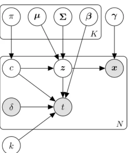
Figure 1: The generative model of VaDeSC.

In this section, we present VaDeSC — the variational deep survival clustering model. Our approach builds on the suc- cess of variational autoencoders (VAEs) (Kingma & Welling, 2014; Rezende et al., 2014) and deep survival analysis (Ran- ganath et al., 2016).

Problem Definition Throughout this paper we will consider the following setting. Let D = {(x

, δ

, t

)}

be a dataset consisting of N triplets, one for each patient. Herein, x

de- notes the explanatory variables, or features. δ

is the censor- ing indicator: δ

= 0 if the survival time of the i-th patient was censored, and δ

= 1 otherwise. Finally, t

is the po- tentially censored survival time. In survival cluster analysis, we additionally consider a latent cluster assignment variable c

∈ {1, ..., K} unobserved at training time. Here, K is the total number of clusters. The problem then is twofold: (i) to discover unobserved cluster assignments and (ii) model the survival distribution given x

and c

.

Generative Model Following the problem definition above, we assume that the data {x

, t

}

are generated from a random process consisting of the following steps. First, the cluster assignment c ∈ {1, . . . , K} is sampled from a categorical distribution. Then, a continuous latent embedding, z ∈ R

, is sampled from a Gaussian distribution, whose mean and variance depend on the se- lected cluster. Explanatory variables x are generated from a distribution conditioned on z, while t depends on the cluster assignment c and latent vector z. The generative process can be then sum- marised as (i) c ∼ p(c; π) = π

; (ii) z ∼ p (z|c; {µ

, ..., µ

} , {Σ

, ..., Σ

}) = N (z; µ

, Σ

);

(iii) x ∼ p(x|z; γ); and (iv) t ∼ p (t|z, c; {β

, ..., β

} , k), where π is a vector of cluster assignment probabilities; µ

and Σ

are mean and variance of the Gaussian distribution corre- sponding to cluster c in the latent space; and β

are cluster-specific survival parameters. Here, p(x|z; γ) = Bernoulli(x; µ

) for binary-valued features and N x; µ

, diag σ

for real- valued features, where µ

and σ

are produced by f(z; γ) – a decoder neural network parame- terised by γ. Figure 1 summarises the random process above graphically.

Survival Model p (t|z, c; {β

, ..., β

} , k) refers to the cluster-specific survival model. Hence- forth, we will use p(t|z, c) as a shorthand notation. We assume that given z and c, the uncen- sored survival time follows the Weibull distribution given by Weibull softplus z

β

, k , where softplus(x) = log (1 + exp(x)) (Ranganath et al., 2016); k is the shape parameter; and β

are cluster-specific survival parameters. Observe that softplus z

β

corresponds to the scale pa- rameter of the Weibull distribution. Although we assume that the shape parameter k is global, an adaptation to cluster-specific parameters, as proposed by Liverani et al. (2020), is straightforward.

Adjusting for right-censoring yields the following distribution:

p(t|z, c) =

"

k λ

t λ

exp − t

λ

!#

"

exp − t

λ

!#

, (1)

where λ

= softplus z

β

.

Joint Probability Distribution Assuming the generative process above, the joint probability of x and t can be written as p(x, t) = R

z

P

c=1

p(x, t, z, c) = R

z

P

c=1

p(x|t, z, c)p(t, z, c). It is important to note that x and t are independent given z, so are x and c. Hence, we can rewrite the joint probability of the data, also referred to as the likelihood function, given the parameters π, µ, Σ, γ, β, k as

p (x, t; π, µ, Σ, γ, β, k) = Z

z K

X

c=1

p(x|z; γ)p(t|z, c; β, k)p(z|c; µ, Σ)p(c; π), (2)

where µ = {µ

, ..., µ

}, Σ = {Σ

, ..., Σ

}, and β = {β

, ..., β

}.

Evidence Lower Bound Since the likelihood function in Equation 2 is intractable, we derive a lower bound of the log marginal probability of the data:

log p(x, t; π, µ, Σ, γ, β, k) ≤ E

log

p(x|z; γ)p(t|z, c; β, k)p(z|c; µ, Σ)p(c; π) q(z, c|x, t)

. (3) We approximate the probability of the latent variables z and c given the observations with a varia- tional distribution q(z, c|x, t) = q(z|x)q(c|z, t), where the first term is the encoder parameterised by a neural network. The second term is set equal-to the true probability p(c|z, t):

q(c|z, t) = p(c|z, t) = p(z, t|c)p(c) P

c=1

p(z, t|c)p(c) = p(t|z, c)p(z|c)p(c) P

c=1

p(t|z, c)p(z|c)p(c) . (4) Thus, the evidence lower bound (ELBO) can be written as

L(x, t) = E

log p(x|z; γ) + log p(t|z, c; β, k) + log p(z|c; µ, Σ) + log p(c; π) − log q(z, c|x, t)

. (5)

In practice, each of the terms of the ELBO in Equation 5 is approximated using the stochastic gradient variational Bayes (SGVB) estimator (Kingma & Welling, 2014). The detailed description is provided in Appendix B.

Missing Survival Time An additional challenge could arise when determining cluster assignments at test-time. Patients’ survival times may not be observable; whereas our derivation of the distribu- tion p(c|z, t) depends on p(t|z, c). Therefore, when the survival time of an individual is unknown, using the Bayes’ rule we compute p(c|z) =

c=1p(z|c)p(c)

. Consequently, we compute the hard cluster assignment as ˆ c = arg max

p(c = ν|z) and the predicted risk as 1/λ

(see Equation 1).

3 R ESULTS

In this section, we compare the proposed VaDeSC model to the semi-supervised clustering (SSC) (Bair & Tibshirani, 2004) and the survival cluster analysis (SCA) (Chapfuwa et al., 2020). Addi- tionally, we include k-means as a na¨ıve clustering baseline. We also consider the regularised Cox PH (Simon et al., 2011) and Weibull AFT models as time-to-event prediction baselines. For the VaDeSC, we perform two ablations: (i) training a completely unsupervised version without mod- elling the survival, which is essentially equivalent to GMMVAE/VaDE, and (ii) predicting cluster assignments when the survival time is unobserved (see Section 2). Further implementation details can be found in Appendix E.

The comparison is performed on a range of (semi-)synthetic and real-world survival datasets with varying numbers of data points, explanatory variables, fractions of censored observations and cluster structures. Appendix C contains a brief summary of all datasets. In particular, we consider synthetic nonlinear data, semi-synthetic survival MNIST (survMNIST) (P¨olsterl, 2019), and real-world SUP- PORT (Knaus et al., 1995) and FLChain (Kyle et al., 2006) data. For (semi-)synthetic data, we focus on the evaluation of the clustering performance in terms of the accuracy (ACC), normalised mutual information (NMI), and adjusted Rand index (ARI) (Emmons et al., 2016). For SUPPORT and FLChain, we compare models w.r.t. time-to-event predictions using the concordance index (CI), relative absolute error (RAE), and calibration slope (CAL, see Appendix D).

Clustering Table 1 shows the results on synthetic and survMNIST data. As can be seen, VaDeSC

outperforms all models in terms of identifying clusters and achieves performance comparable to

SCA w.r.t. the CI. Interestingly, SCA completely fails to identify clusters correctly on synthetic data,

for which the generative process is very similar to the one assumed by VaDeSC. In the synthetic data,

the clusters do not have prominently different survival distributions: they are rather characterised by

differences in the association between the covariates and survival times. This could explain the

poor performance of SCA which tends to discover clusters with disparate survival distributions. It

appears that SSC offers little to no gain over the k-means based on all features. In both datasets,

we see that including survival times results in considerable clustering performance improvements, and the unsupervised variant of VaDeSC performs significantly worse than the full model. Overall, these results suggest that VaDeSC compares favourably to the related methods at clustering survival data.

Table 1: Test set performance on synthetic and survMNIST data. Averages and standard deviations are reported across 5 and 10 independent simulations, respectively. Best results are shown in bold, second best – in italic. Training set results can be found in Appendix F.

Dataset Method ACC NMI ARI CI

Synthetic

k-means 0.44±0.04 0.06±0.04 0.05±0.03 —

Cox PH — — — 0.77±0.02

SSC 0.45±0.03 0.08±0.04 0.06±0.02 —

SCA 0.45±0.09 0.05±0.05 0.04±0.05 0.82±0.02 Ours (w/o surv.) 0.74±0.21 0.53±0.12 0.55±0.20 — Ours (w/o t) 0.88±0.03 0.60±0.07 0.67±0.07

Ours 0.90±0.02 0.66±0.05 0.73±0.05 0.84±0.02

survMNIST

k-means 0.49±0.06 0.31±0.04 0.22±0.04 —

Cox PH — — — 0.74±0.04

SSC 0.49±0.06 0.31±0.04 0.22±0.04 —

SCA 0.56±0.09 0.46±0.06 0.33±0.10 0.79±0.06 Ours (w/o surv.) 0.47±0.07 0.38±0.08 0.24±0.08 — Ours (w/o t) 0.57±0.09 0.51±0.09 0.37±0.10

Ours 0.58±0.10 0.55±0.11 0.39±0.11 0.80±0.05

Time-to-event Prediction Table 2 shows time-to-event prediction results on SUPPORT and FLChain datasets. RAE was evaluated based on the predicted median survival times. Observe that overall VaDeSC performs comparably to the Weibull AFT and SCA models, even achieving the best average results on SUPPORT. Surprisingly, SCA has a considerable variance w.r.t. the calibration slope, sometimes yielding badly calibrated predictions. Note that for SCA, the obtained results differ from the ones reported by Chapfuwa et al. (2020) likely due to differences in encoder architectures and numbers of latent dimensions. On FLChain, SCA achieves a considerably better calibration than the other two models, however, this is not surprising given that it optimises calibration explicitly.

Table 2: Test set performance on SUPPORT and FLChain datasets. Averages and standard devia- tions are reported across 5 train-test splits. Best results are shown in bold.

Dataset Method CI RAE CAL

SUPPORT

Weibull AFT 0.84±0.01 0.62±0.01 1.27±0.02 SCA 0.83±0.02 0.78±0.13 1.74±0.52 Ours 0.85±0.01 0.53±0.02 1.24±0.05 FLChain

Weibull AFT 0.80±0.01 0.72±0.01 2.18±0.07 SCA 0.78±0.02 0.69±0.08 1.33±0.24 Ours 0.80±0.01 0.76±0.01 2.52±0.08

4 C ONCLUSION

In this paper, we introduced a novel deep probabilistic model for clustering survival data. In contrast to existing approaches, our method can retrieve clusters of patients regulated by different survival models and it can be trained efficiently in the framework of stochastic gradient variational inference.

Empirically, we show that our model offers an improvement in clustering performance compared to the related work while staying competitive at time-to-event modelling.

Future Work Some further directions of work include introducing interpretable explanations of

our model’s predictions to facilitate its application in the medical domain; a fully Bayesian treat-

ment of global parameters to alleviate the need for a fixed number of clusters; and the inclusion of

more complex datasets. It would also be interesting to evaluate and compare obtained clustering

qualitatively, since the performance metrics considered so far do not fully reflect all aspects of the

underlying problem.

R EFERENCES

M. Abadi, A. Agarwal, P. Barham, E. Brevdo, Z. Chen, C. Citro, G. S. Corrado, A. Davis, J. Dean, M. Devin, S. Ghemawat, I. Goodfellow, A. Harp, G. Irving, M. Isard, Y. Jia, R. Jozefow- icz, L. Kaiser, M. Kudlur, J. Levenberg, D. Man´e, R. Monga, S. Moore, D. Murray, C. Olah, M. Schuster, J. Shlens, B. Steiner, I. Sutskever, K. Talwar, P. Tucker, V. Vanhoucke, V. Va- sudevan, F. Vi´egas, O. Vinyals, P. Warden, M. Wattenberg, M. Wicke, Y. Yu, and X. Zheng.

TensorFlow: Large-scale machine learning on heterogeneous systems, 2015. URL http:

//tensorflow.org/.

E. Ahlqvist, P. Storm, A. K¨ar¨aj¨am¨aki, M. Martinell, M. Dorkhan, A. Carlsson, P. Vikman, R. B.

Prasad, D. M. Aly, P. Almgren, Y. Wessman, N. Shaat, P. Sp´egel, H. Mulder, E. Lindholm, O. Melander, O. Hansson, U. Malmqvist, ˚ A. Lernmark, K. Lahti, T. Fors´en, T. Tuomi, A. H.

Rosengren, and L. Groop. Novel subgroups of adult-onset diabetes and their association with outcomes: a data-driven cluster analysis of six variables. The Lancet Diabetes & Endocrinology, 6(5):361–369, 2018.

E. Bair and R. Tibshirani. Semi-supervised methods to predict patient survival from gene expression data. PLoS Biology, 2(4):e108, 2004.

J. Buckley and I. James. Linear regression with censored data. Biometrika, 66(3):429–436, 1979.

P. Chapfuwa, C. Tao, C. Li, C. Page, B. Goldstein, L. C. Duke, and R. Henao. Adversarial time- to-event modeling. In Proceedings of the 35th International Conference on Machine Learning, volume 80, pp. 735–744. PMLR, 2018.

P. Chapfuwa, C. Li, N. Mehta, L. Carin, and R. Henao. Survival cluster analysis. In Proceedings of the ACM Conference on Health, Inference, and Learning, pp. 60–68. Association for Computing Machinery, 2020.

F. S. Collins and H. Varmus. A new initiative on precision medicine. New England Journal of Medicine, 372(9):793–795, 2015.

D. R. Cox. Regression models and life-tables. Journal of the Royal Statistical Society: Series B (Methodological), 34(2):187–202, 1972.

D. G. Altman. Analysis of survival times. In Practical Statistics for Medical Research, chapter 13, pp. 365–395. Chapman and Hall/CRC Texts in Statistical Science Series, 2020.

C. Davidson-Pilon, J. Kalderstam, N. Jacobson, S. Reed, B. Kuhn, P. Zivich, M. Williamson, J. K.

Abdeali, D. Datta, A. Fiore-Gartland, A. Parij, D. Wilson, Gabriel, L. Moneda, A. Moncada- Torres, K. Stark, H. Gadgil, Jona, K. Singaravelan, L. Besson, M. Sancho Pe˜na, S. Anton, A. Klintberg, J. Growth, J. Noorbakhsh, M. Begun, R. Kumar, S. Hussey, S. Seabold, and D. Gol- land. lifelines: v0.25.9, 2021. URL https://doi.org/10.5281/zenodo.4505728.

N. Dilokthanakul, P. A. M. Mediano, M. Garnelo, M. C. H. Lee, H. Salimbeni, K. Arulkumaran, and M. Shanahan. Deep unsupervised clustering with Gaussian mixture variational autoencoders, 2016. arXiv:1611.02648.

A. Dispenzieri, J. A. Katzmann, R. A. Kyle, D. R. Larson, T. M. Therneau, C. L. Colby, R. J. Clark, G. P. Mead, S. Kumar, L. J. Melton, and S. V. Rajkumar. Use of nonclonal serum immunoglobulin free light chains to predict overall survival in the general population. Mayo Clinic Proceedings, 87(6):517–523, 2012.

S. Emmons, S. Kobourov, M. Gallant, and K. B¨orner. Analysis of network clustering algorithms and cluster quality metrics at scale. PLOS ONE, 11(7):e0159161, 2016.

D. Faraggi and R. Simon. A neural network model for survival data. Statistics in Medicine, 14(1):

73–82, 1995.

V. T. Farewell. The use of mixture models for the analysis of survival data with long-term survivors.

Biometrics, 38(4):1041–1046, 1982.

D. A. Fenstermacher, R. M. Wenham, D. E. Rollison, and W. S. Dalton. Implementing personalized medicine in a cancer center. The Cancer Journal, 17(6):528–536, 2011.

H. Ishwaran, U. B. Kogalur, E. H. Blackstone, and M. S. Lauer. Random survival forests. Annals of Applied Statistics, 2(3):841–860, 2008.

R. A. Jacobs, M. I. Jordan, S. J. Nowlan, and G. E. Hinton. Adaptive mixtures of local experts.

Neural Computation, 3(1):79–87, 1991.

Z. Jiang, Y. Zheng, H. Tan, B. Tang, and H. Zhou. Variational deep embedding: An unsupervised and generative approach to clustering. In Proceedings of the 26th International Joint Conference on Artificial Intelligence, pp. 1965–1972. AAAI Press, 2017.

M. J. Johnson, D. K. Duvenaud, A. Wiltschko, R. P. Adams, and S. R. Datta. Composing graphical models with neural networks for structured representations and fast inference. In Advances in Neural Information Processing Systems, volume 29, pp. 2946–2954. Curran Associates, Inc., 2016.

J. L. Katzman, U. Shaham, A. Cloninger, J. Bates, T. Jiang, and Y. Kluger. DeepSurv: Personalized treatment recommender system using a Cox proportional hazards deep neural network. BMC Medical Research Methodology, 18(1), 2018.

D. P. Kingma and M. Welling. Auto-encoding variational Bayes. In 2nd International Conference on Learning Representations, 2014.

W. A. Knaus, F. E. Harrell, J. Lynn, L. Goldman, R. S. Phillips, A. F. Connors, N. V. Dawson, W. J.

Fulkerson, R. M. Califf, N. Desbiens, P. Layde, R. K. Oye, P. E. Bellamy, R. B. Hakim, and D. P. Wagner. The SUPPORT prognostic model: Objective estimates of survival for seriously ill hospitalized adults. Annals of Internal Medicine, 122(3):191–203, 1995.

H. Kvamme, Ø. Borgan, and I. Scheel. Time-to-event prediction with neural networks and Cox regression. Journal of Machine Learning Research, 20(129):1–30, 2019.

R. A. Kyle, T. M. Therneau, S. V. Rajkumar, D. R. Larson, M. F. Plevak, J. R. Offord, A. Dispenzieri, J. A. Katzmann, and L. J. Melton. Prevalence of monoclonal gammopathy of undetermined significance. New England Journal of Medicine, 354(13):1362–1369, 2006.

Y. LeCun, C. Cortes, and C. J. Burges. MNIST handwritten digit database. ATT Labs, 2, 2010. URL http://yann.lecun.com/exdb/mnist.

S. Liverani, L. Leigh, I. L. Hudson, and J. E. Byles. Clustering method for censored and collinear survival data. Computational Statistics, 2020.

Y. Luo, T. Tian, J. Shi, J. Zhu, and B. Zhang. Semi-crowdsourced clustering with deep generative models. In Advances in Neural Information Processing Systems, volume 31, pp. 3212–3222.

Curran Associates, Inc., 2018.

G. J. McLachlan and D. Peel. Finite mixture models. John Wiley & Sons, 2004.

E. Min, X. Guo, Q. Liu, G. Zhang, J. Cui, and J. Long. A survey of clustering with deep learning:

From the perspective of network architecture. IEEE Access, 6:39501–39514, 2018.

J. Molitor, M. Papathomas, M. Jerrett, and S. Richardson. Bayesian profile regression with an application to the national survey of children’s health. Biostatistics, 11(3):484–498, 2010.

S. C. Mouli, B. Ribeiro, and J. Neville. A deep learning approach for survival clustering without end-of-life signals, 2018. URL https://openreview.net/forum?id=SJme6-ZR-.

C. Nagpal, X. R. Li, and A. Dubrawski. Deep survival machines: Fully parametric survival re- gression and representation learning for censored data with competing risks. IEEE Journal of Biomedical and Health Informatics, 2021a.

C. Nagpal, S. Yadlowsky, N. Rostamzadeh, and K. Heller. Deep Cox mixtures for survival regres-

sion, 2021b. arXiv:2101.06536.

F. Pedregosa, G. Varoquaux, A. Gramfort, V. Michel, B. Thirion, O. Grisel, M. Blondel, P. Pretten- hofer, R. Weiss, V. Dubourg, J. Vanderplas, A. Passos, D. Cournapeau, M. Brucher, M. Perrot, and E. Duchesnay. Scikit-learn: Machine learning in Python. Journal of Machine Learning Research, 12:2825–2830, 2011.

S. P¨olsterl. Survival analysis for deep learning, 2019. URL https://k-d-w.org/blog/

2019/07/survival-analysis-for-deep-learning/.

R Core Team. R: A Language and Environment for Statistical Computing. R Foundation for Statis- tical Computing, Vienna, Austria, 2020. URL https://www.R-project.org/.

R. Ranganath, A. Perotte, N. Elhadad, and D. Blei. Deep survival analysis. In Proceedings of the 1st Machine Learning for Healthcare Conference, volume 56, pp. 101–114. PMLR, 2016.

V. C. Raykar, H. Steck, B. Krishnapuram, C. Dehing-Oberije, and P. Lambin. On ranking in survival analysis: Bounds on the concordance index. In Proceedings of the 20th International Conference on Neural Information Processing Systems, pp. 1209–1216. Curran Associates Inc., 2007.

D. J. Rezende, S. Mohamed, and D. Wierstra. Stochastic backpropagation and approximate infer- ence in deep generative models. In Proceedings of the 31st International Conference on Machine Learning, volume 32, pp. 1278–1286. PMLR, 2014.

R. Rodr´ıguez. Lecture notes on generalized linear models, 2007. URL https://data.

princeton.edu/wws509/notes/.

O. Rosen and M. Tanner. Mixtures of proportional hazards regression models. Statistics in Medicine, 18(9):1119–1131, 1999.

N. Simon, J. Friedman, T. Hastie, and R. Tibshirani. Regularization paths for Cox's proportional hazards model via coordinate descent. Journal of Statistical Software, 39(5), 2011.

J. Tanniou, I. van der Tweel, S. Teerenstra, and K. C. B. Roes. Subgroup analyses in confirmatory clinical trials: time to be specific about their purposes. BMC Medical Research Methodology, 16 (1), 2016.

L. van der Maaten and G. Hinton. Visualizing data using t-SNE. Journal of Machine Learning Research, 9(86):2579–2605, 2008.

E. Xia, X. Du, J. Mei, W. Sun, S. Tong, Z. Kang, J. Sheng, J. Li, C. Ma, J. Dong, and S. Li.

Outcome-driven clustering of acute coronary syndrome patients using multi-task neural network with attention, 2019. arXiv:1903.00197.

C.-N. Yu, R. Greiner, H.-C. Lin, and V. Baracos. Learning patient-specific cancer survival distri-

butions as a sequence of dependent regressors. In Advances in Neural Information Processing

Systems, volume 24. Curran Associates, Inc., 2011.

A R ELATED W ORK

Herein, we provide a detailed overview of the related work. The proposed VaDeSC model (see Section 2) builds on three major topics: probabilistic deep unsupervised clustering, mixtures of regression models, and survival analysis. In addition, we discuss several recent close lines of work focusing on clustering survival data.

Deep Unsupervised Clustering Clustering methods have been recently combined with deep neu- ral networks to learn better representations of high-dimensional data (Min et al., 2018). Several techniques have been proposed in the literature, featuring a wide range of neural network architec- tures, such as autoencoders (AE), feed-forward networks, generative adversarial networks (GAN), and variational autoencoders (VAE).

The VAE (Kingma & Welling, 2014; Rezende et al., 2014) combines variational Bayesian methods with the flexibility and scalability of neural networks. Gaussian mixture variational autoencoders (GMMVAE) and variational deep embedding (VaDE) (Dilokthanakul et al., 2016; Jiang et al., 2017) are variants of the VAE in which the prior is a Gaussian mixture distribution. With this assumption, the data is clustered in the latent space of the VAE and the resulting inference model can be directly optimised within the framework of stochastic gradient variational Bayes. Further extensions focus on a fully Bayesian treatment of global parameters with a Dirichlet prior over the mixing coefficients of the Gaussian mixture model (GMM) (Luo et al., 2018; Johnson et al., 2016), alleviating the need to fix the number of clusters a priori.

Mixtures of Regression Models Mixtures of regression (McLachlan & Peel, 2004) model a re- sponse variable by a mixture of individual regressions with the help of latent cluster assignments.

Such mixtures do not have to be limited to a finite number of components; for example, profile re- gression (Molitor et al., 2010) leverages the Dirichlet mixture model for cluster assignment. Along similar lines, within the machine learning community, mixture of experts models (MoE) were intro- duced by Jacobs et al. (1991).

Nonlinear Survival Analysis One of the first machine learning approaches for survival analysis was Faraggi-Simon’s network (Faraggi & Simon, 1995), which was an extension of the classical Cox PH model (Cox, 1972). Since then, an abundance of machine learning methods have been developed: random survival forests (Ishwaran et al., 2008), deep survival analysis (Ranganath et al., 2016), neural networks based on the Cox PH model (Katzman et al., 2018; Kvamme et al., 2019), adversarial time-to-event modelling (Chapfuwa et al., 2018), and deep survival machines (Nagpal et al., 2021a). Of particular interest is the deep survival analysis (DSA) model which similar to our approach (see Section 2), relies on learning latent representations and modelling the survival time with a Weibull distribution (Ranganath et al., 2016).

Mixture models mentioned above have been leveraged for survival analysis as well (Farewell, 1982;

Rosen & Tanner, 1999; Nagpal et al., 2021b). For instance, Farewell (1982) considered fitting sep- arate models for two subpopulations: short-term and long-term survivors. Rosen & Tanner (1999) extended the classical Cox PH model with the MoE. A more recent approach of deep Cox mixtures (DCM), introduced by Nagpal et al. (2021b), fits a finite mixture of Cox regression models on rich representations produced by an encoding neural network.

Clustering Survival Data Clustering of survival data has remained a relatively under-explored

area. Bair & Tibshirani (2004) propose pre-selecting variables based on univariate Cox regression

hazard scores and subsequently performing k-means clustering on the subset of features to discover

patient subpopulations. Ahlqvist et al. (2018) use Cox regression to explore differences across

subgroups of diabetic patients discovered by k-means and hierarchical clustering. In the spirit of

Farewell (1982), Mouli et al. (2018) propose a deep clustering approach to differentiate between

long-term and short-term survivors based on a modified Kuiper statistic in absence of end-of-life

signals. Xia et al. (2019) adapt a multitask learning approach for the outcome-driven clustering of

acute coronary syndrome patients. Liverani et al. (2020) propose a clustering method for collinear

survival data based on the profile regression. They introduce a Dirichlet process mixture model with

cluster-specific parameters for the Weibull distribution. Last but not least, Chapfuwa et al. (2020)

propose outcome-driven survival cluster analysis (SCA) based on a truncated Dirichlet process and neural networks for the encoder and time-to-event prediction model.

Comparison to VaDeSC The proposed variational deep survival clustering (VaDeSC) method (see Section 2) differs from the previously introduced techniques in several ways. Table 3 sum- marises key differences across the models most closely related to VaDeSC. In brief, deep survival analysis (Ranganath et al., 2016) is merely a survival analysis model and does not perform clus- tering. Semi-supervised clustering (Bair & Tibshirani, 2004) does not tackle time-to-event predic- tion directly and relies on k-means which limits its applicability to more complex and unstructured datasets. While the approach by Liverani et al. (2020) is quite similar to VaDeSC, it does not learn low-dimensional representations and relies on Markov chain Monte Carlo (MCMC) methods for fitting which have limited scalability. Last but not least, survival cluster analysis (Chapfuwa et al., 2020) is not equipped with a decoder arm and thus, only maximises the likelihood of survival time alone.

Table 3: Comparison of the proposed VaDeSC model to the related approaches: deep survival anal- ysis (DSA), semi-supervised clustering (SSC), profile regression for survival data, and survival clus- ter analysis (SCA). Here, t denotes survival time, x denotes explanatory variables, z corresponds to latent representations, and K stands for the number of clusters.

DSA

Ranganath et al. (2016)

SSC

Bair & Tibshirani (2004)

Profile Regression

Liverani et al. (2020)

SCA

Chapfuwa et al. (2020)

Ours Performs

clustering? 7 3 3 3 3

Predicts t? 3 7 3 3 3

Learns z? 3 7 7 3 3

Maximises the likelihood of x and t jointly?

7 7 3 7 3

Infers a simple link between x/z and t?

3 7 3 7 3

Scales to un-

structured data? 3 7 7 3 3

Optimises

calibration? 7 7 7 3 7

Does not require a fixed K a priori?

— 7 3 3 7

B ELBO T ERMS

Below we explain how each term of the ELBO from Equation 5 can be optimized using Monte Carlo sampling and stochastic gradient descent.

Reconstruction The reconstruction term can be approximated using the SGVB estimator (Kingma

& Welling, 2014). We use the same principle for the rest of the terms. Herein, we provide the derivation for p(x|z; γ) = Bernoulli(x; µ

), i.e. for binary-valued explanatory variables:

E

log p(x|z; γ) = E

log p(x|z; γ) ≈ 1 L

L

X

l=1

log p(x|z

; γ)

= 1 L

L

X

l=1 D

X

d=1

x

log µ

+ (1 − x

) log(1 − µ

),

(6)

where L is the number of Monte Carlo samples in the SGVB estimator; µ

= f (z

; γ), z

∼ q(z|x) = N (z; µ

, σ

), [µ

, log σ

] = g(x; θ) and g(·; θ) is an encoder neural network parameterised by θ; x

refers to the d-th component of x and D is the number of features. For other data types, the distribution p(x|z; γ) in Equation 6 needs to be adjusted accordingly.

Survival The second term of the ELBO includes the survival time. Following the survival model described by Equation 1, the SGVB estimator for the term is given by

E

logp(t|z, c; β, k) ≈

L

X

l=1 K

X

ν=1

log p(t|z

, c = ν ; β, k)p(c = ν |z

, t)

= 1 L

L

X

l=1 K

X

ν=1

log



 ( k

λ

t

λ

)

exp − t

λ

! 

 p(c = ν |z

, t), (7)

where λ

= softplus z

β

.

Clustering The third term in Equation 5 corresponds to the clustering loss and is defined as E

log p(z|c; µ, Σ) = E

K

X

ν=1

p(c = ν|z, t) log p(z|c = ν; µ, Σ)

≈ 1 L

L

X

l=1 K

X

ν=1

p(c = ν |z

, t) log p(z

|c = ν ; µ, Σ).

(8)

Prior The fourth term can be approximated as E

log p(c; π) ≈ 1

L

L

X

l=1 K

X

ν=1

p(c = ν |z

, t) log p(c = ν ; π). (9) Variational Finally, the fifth term of the ELBO corresponds to the entropy of the variational dis- tribution q(z, c|x, t):

− E

log q(z, c|x, t) = E

[log q(z|x) + log p(c|z, t)]

= − E

log q(z|x) − E

log p(c|z, t), (10) where the first term is the entropy of a multivariate Gaussian distribution with a diagonal covariance matrix. We can then approximate the expression in Equation 10 by

J

2 (log(2π) + 1) +

J

X

j=1

log σ

− 1 L

L

X

l=1 K

X

ν=1

p(c = ν|z

, t) log p(c = ν|z

, t), (11) where J is the number of latent space dimensions.

C D ATASETS

In Table 4 we provide an overview of the datasets used in the experiments. In the following, we describe each dataset in details.

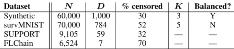
Table 4: Summary of the datasets. N is the total number of data points, including train and test sets, D is the number of explanatory variables (including dummy variables), K is the number of clusters (if known). We report the average percentage of censored observations across all simulations and whether the cluster sizes are balanced (if known).

Dataset N D % censored K Balanced?

Synthetic 60,000 1,000 30 3 Y

survMNIST 70,000 784 52 5 N

SUPPORT 9,105 59 32 — —

FLChain 6,524 7 70 — —

C.1 S YNTHETIC D ATA

Herein, we provide details on the generation of synthetic survival data used in our experiments (see Section 3). The procedure for simulating these data is very similar to the generative process assumed by the proposed VaDeSC model (cf. Section 2) and can be summarised as follows:

1. Let π

=

, for 1 ≤ c ≤ K.

2. Sample c

∼ Cat(π), for 1 ≤ i ≤ N . 3. Sample µ

∼ unif −

,

, for 1 ≤ c ≤ K and 1 ≤ j ≤ J.

4. Let Σ

= I

S

, where S

∈ R

is a random symmetric, positive-definite matrix,

for 1 ≤ c ≤ K.

5. Sample z

∼ N (µ

, Σ

), for 1 ≤ i ≤ N.

6. Let g

(z) = W

ReLU (W

ReLU (W

z + b

) + b

) + b

, where W

∈ R

, W

∈ R

, W

∈ R

and b

∈ R

, b

∈ R

, b

∈ R

are random matrices and vectors,

and h is the number of hidden units.

7. Let x

= g

(z

), for 1 ≤ i ≤ N.

8. Sample β

∼ unif (−10, 10), for 1 ≤ c ≤ K and 0 ≤ j ≤ J . 9. Sample u

∼ Weibull softplus z

β

, k

,

for 1 ≤ i ≤ N . 10. Sample δ

∼ Bernoulli(1 − p

), for 1 ≤ i ≤ N.

11. Let t

= u

if δ

= 1, and sample t

∼ unif(0, u

) otherwise, for 1 ≤ i ≤ N .

Here, similar to Section 2, K is the number of clusters; N is the number of data points; J is the number of latent variables; D is the number of features; k is the shape parameter of the Weibull distribution (see Equation 1); and p

denotes the probability of censoring. The key difference between clusters is in how latent variables z generate the survival time t: each cluster has a different weight vector β that determines the scale of the Weibull distribution.

In our experiments, we fix K = 3, N = 60000, J = 16, D = 1000, k = 1, and p

= 0.3. We hold out 18000 data points as a test set and repeat simulations 5 times independently. A visualisation of one simulation is shown in Figure 2. As can be seen in the t-SNE (van der Maaten & Hinton, 2008) plot, three clusters are not as clearly separable based on covariates alone; on the other hand, they have visibly distinct survival curves as shown in the Kaplan–Meier plot.

(a) t-SNE plot. (b) Kaplan–Meier plot.

Figure 2: Visualisation of one replicate of the synthetic data. t-SNE plot (on the left) is based on the explanatory variables only. Kaplan–Meier curves (on the right) are plotted separately for each cluster. Different colours correspond to different clusters.

1

Generated using make spd matrix from scikit-learn (Pedregosa et al., 2011).

2

W

, W

, W

are generated using make low rank matrix from scikit-learn (Pedregosa et al., 2011).

3

We omitted bias terms for the sake of brevity.

C.2 S URVIVAL MNIST D ATA

We generate semi-synthetic survMNIST data as described by P¨olsterl (2019).

The generative pro- cess can be summarised by the following steps:

1. Assign every digit in the original MNIST dataset (LeCun et al., 2010) to one of K clusters (ensure that every cluster contains at least one digit)

2. Sample risk score r

∼ unif

, 15

, for 1 ≤ c ≤ K.

3. Let λ

=

0

exp(r

), for 1 ≤ c ≤ K, where T

is the specified mean survival time and

is the baseline hazard.

4. Sample a

∼ unif(0, 1) and let u

= −

ci

, for 1 ≤ i ≤ N.

5. Let q

= q

(u

), where q

(·) denotes the α-th quantile.

6. Sample t

∼ unif (min

u

, q

).

7. Let δ

= 1 if u

≤ t

, and δ

= 0 otherwise, for 1 ≤ i ≤ N . 8. Let t

= u

if δ

= 1, and t

= t

otherwise, for 1 ≤ i ≤ N .

Herein, the notation is the same as in Appendix C.1. It is important to note that as opposed to the synthetic data, in survMNIST censoring is not independent from the uncensored survival time, since individuals with larger survival times are more likely to be censored. Moreover, observe that here p

is only a lower bound on the probability of censoring and the fraction of censored observations can be much larger than p

. In this sense, the survMNIST dataset violates assumptions of the conventional survival analysis models.

In our experiments, we fix K = 5 and p

= 0.3. We repeat simulations independently 10 times.

The train-test split is defined as in the original MNIST data (60,000 vs. 10,000). Table 5 shows an example of cluster and risk score assignments in one of the simulations. The resulting dataset is visualised in Figure 3. Observe that the clusters are not well-distinguishable based on covariates alone. Also note that some clusters contain many censored data points, whereas some do not contain any, as shown in the Kaplan–Meier plot.

Table 5: An example of an assignment of MNIST digits to clusters and risk scores under K = 5.

Digit Cluster Risk Score

0 2 13.12

1 3 5.17

2 4 11.60

3 2 13.12

4 1 7.62

5 5 2.03

6 2 13.12

7 4 11.60

8 1 7.62

9 3 5.17

4

Based on the original implementation available at

https://github.com/sebp/survival-cnn-estimator .

(a) t-SNE plot. (b) Kaplan–Meier plot.

Figure 3: Visualisation of one replicate of the survMNIST dataset.

C.3 SUPPORT & FLC HAIN

The Study to Understand Prognoses and Preferences for Outcomes and Risks of Treatments (SUP- PORT) (Knaus et al., 1995) consists of seriously ill hospitalised adults from five tertiary care aca- demic centres in the United States. It includes demographic, laboratory, and scoring data acquired from patients diagnosed with cancer, chronic obstructive pulmonary disease, congestive heart fail- ure, cirrhosis, acute renal failure, multiple organ system failure, and sepsis. In this dataset, we impute missing entries with medians and modes for numerical and categorical features, respectively.

This dataset is publicly available.

The study of the relationship between serum free light chain (FLChain) and mortality (Kyle et al., 2006; Dispenzieri et al., 2012) was conducted in Olmsted County, Minnesota in the United States.

The dataset includes demographic and laboratory variables alongside with the recruitment year. In our analysis, we omit all patients with missing features. FLChain is by far the most heavily censored and low-dimensional among the considered datasets (see Table 4). Similar to SUPPORT, FLChain data are publicly available.

D E VALUATION M ETRICS

For clustering performance, we employ ARI and NMI as implemented in the sklearn.metrics module of scikit-learn (Pedregosa et al., 2011). Clustering accuracy is evaluated by finding an optimal mapping between assignments and true cluster labels using the Hungarian algorithm, as implemented in sklearn.utils.linear assignment .

The concordance index (Raykar et al., 2007) evaluates how well a survival model is able to rank individuals in terms of their risk. Given observed survival times t

, predicted risk scores η

, and censoring indicators δ

, the concordance index is defined as

CI = P

i=1

P

j=1

1

1

δ

P

P

j=1

1

δ

. (12)

Thus, a perfect ranking achieves a CI of 1.0, whereas a random ranking is expected to have a CI of 0.5. We use the lifelines implementation of the CI (Davidson-Pilon et al., 2021).

Relative absolute error (Yu et al., 2011) evaluates predicted survival times in terms of their relative deviation from the observed survival times. In particular, given predicted survival times ˆ t

, RAE is defined as

RAE = P

i=1

ˆ t

− t

/ ˆ t

δ

P

δ

. (13)

Note that we only evaluate RAE on uncensored observations.

Last but not least, similar to Chapfuwa et al. (2020) we use the calibration slope to evaluate the

calibration of models. It is desirable for the predicted survival times to match with the empirical

marginal distribution of t. Calibration slope indicates whether a model tends to under- or overesti- mate risk on average, and thus, an ideal calibration slope is 1.0. We use the implementation by Chap- fuwa et al. (2020) available at https://github.com/paidamoyo/survival_cluster_

analysis.

E I MPLEMENTATION D ETAILS

Herein, we provide implementation details for the experiments described in Section 3.

For all datasets, we re-scale survival times to be in [0.001, 1.001]. For survMNIST we re-scale the features to be in [0, 1]. For the other datasets, we re-scale the features to zero-mean and unit-variance.

Categorical features are encoded using dummy variables.

We implemented the VaDeSC model in TensorFlow (Abadi et al., 2015). Currently, the code is only available on request. We use two different architectures for encoders and decoders as described in Tables 6 and 7. Hyperparameters across all datasets are reported in Table 8. We use L = 1 Monte Carlo samples for the SGVB estimator (see Appendix B). As opposed to many unsupervised clustering methods, we do not pre-train autoencoder weights. Generally, we observe little variability in performance when varying the number of latent dimensions, shape of the Weibull distribution or mini-batch size.

Semi-supervised Clustering We re-implemented SSC in Python based on the R code (R Core Team, 2020) provided by Bair & Tibshirani (2004). Since SSC requires specifying a threshold for selecting a subset of features for k-means clustering, we report the best results achieved w.r.t. NMI across a range of thresholds.

Survival Cluster Analysis We use the original implementation of SCA available at https:

//github.com/paidamoyo/survival_cluster_analysis. To facilitate a fair com- parison to VaDeSC, we use the same architectures for the encoder (see Tables 6 and 7) and the same numbers of latent dimensions (see Table 8). We truncate the Dirichlet process at the true number of clusters for synthetic and survMNIST data. For SUPPORT and FLChain, we set the maximum number of cluster at K = 25. For all datasets, we use a concentration parameter of 2.0. We train the model for 300 epochs on survMNIST and synthetic data and for 400 and 600 epochs on SUPPORT and FLChain, respectively.

Other Baselines For Cox PH and Weibull AFT models, we use the implementation in lifelines

(Davidson-Pilon et al., 2021). We use penalised versions of these models by setting the penalty

weight to 0.01. To avoid numerical instability, we remove all features with variance close to 0. For

k-means clustering, we use the scikit-learn implementation (Pedregosa et al., 2011).

Table 6: Encoder and decoder architectures used for synthetic and survMNIST data. tfkl stands for tensorflow.keras.layers. encoded size corresponds to the number of latent di- mensions, J ; and inp shape is the number of input dimesions, D. For survMNIST, the activation of the last decoder layer is set to ’sigmoid’.

Encoder

1 tfkl.Dense(500, activation=’relu’) 2 tfkl.Dense(500, activation=’relu’) 3 tfkl.Dense(2000, activation=’relu’)

4 mu = tfkl.Dense(encoded size, activation=None);

sigma = tfkl.Dense(encoded size, activation=None)

Decoder

1 tfkl.Dense(2000, activation=’relu’) 2 tfkl.Dense(500, activation=’relu’) 3 tfkl.Dense(500, activation=’relu’) 4 tfkl.Dense(inp shape)

Table 7: Encoder and decoder architectures used for SUPPORT and FLChain data.

Encoder

1 tfkl.Dense(50, activation=’relu’) 2 tfkl.Dense(100, activation=’relu’)

3 mu = tfkl.Dense(encoded size, activation=None);

sigma = tfkl.Dense(encoded size, activation=None)

Decoder

1 tfkl.Dense(100, activation=’relu’) 2 tfkl.Dense(50, activation=’relu’) 3 tfkl.Dense(inp shape)

Table 8: Hyperparameters used for training the VaDeSC across all datasets. Herein, J denotes the number of latent dimensions; K is the number of clusters; and k is the shape parameter of the Weibull distribution. MSE stands for mean squared error; CE – for cross entropy.

Dataset J K k Mini-batch

Size

Learning

Rate # epochs Reconstruction Loss

Synthetic 16 3 1.0 256 0.001 1,000 MSE

survMNIST 16 5 1.0 256 0.001 300 Binary CE

SUPPORT 16 4 2.0 256 0.001 300 MSE

FLChain 4 2 2.0 256 0.001 300 MSE

F F URTHER R ESULTS

Table 9: Training set performance on synthetic and survMNIST data. Averages and standard devia- tions are reported across 5 and 10 independent simulations, respectively. Best results are shown in bold, second best in italic.

Dataset Method ACC NMI ARI CI

Synthetic

k-means 0.44±0.04 0.06±0.04 0.05±0.03 —

Cox PH — — — 0.78±0.02

SSC 0.44±0.02 0.08±0.04 0.06±0.02 —

SCA 0.45±0.09 0.05±0.05 0.05±0.05 0.83±0.02 Ours (w/o surv.) 0.73±0.21 0.53±0.12 0.55±0.21 — Ours (w/o t) 0.88±0.03 0.60±0.07 0.67±0.07

Ours 0.90±0.02 0.66±0.05 0.74±0.05 0.85±0.01

survMNIST

k-means 0.48±0.06 0.30±0.04 0.21±0.04 —

Cox PH — — — 0.77±0.05

SSC 0.48±0.06 0.30±0.04 0.21±0.04 —

SCA 0.56±0.09 0.47±0.07 0.34±0.11 0.83±0.05 Ours (w/o surv.) 0.47±0.07 0.38±0.08 0.24±0.07 — Ours (w/o t) 0.57±0.10 0.52±0.10 0.37±0.10

Ours 0.58±0.10 0.54±0.12 0.39±0.11 0.83±0.06