Introduction to fuzzy control

Educational Material

Introduction to fuzzy control

Author(s):

Geering, Hans P.

Publication Date:

1998

Permanent Link:

https://doi.org/10.3929/ethz-a-004953512

Rights / License:

In Copyright - Non-Commercial Use Permitted

This page was generated automatically upon download from the ETH Zurich Research Collection. For more information please consult the Terms of use.

ETH Library

Introduction to Fuzzy Control

Hans P. Geering

Abstract

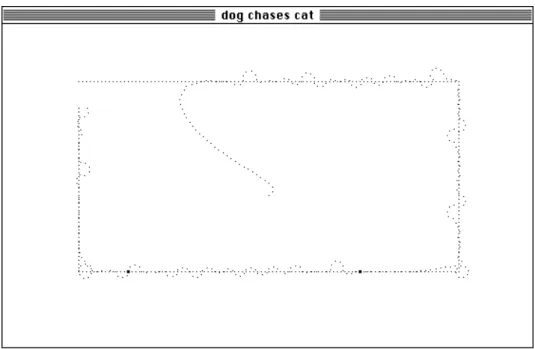
In this report, some of the basic mathematical definitions and rules of fuzzy system theory are described inasmuch as they are relevant for fuzzy control. Two examples are covered in detail, viz., a fuzzy closed- loop halting control scheme for the forward motion of a mobile robot in an automatic factory and a dog chasing a cat using fuzzy control.

Issues of computational efficiency are discussed. And some recommen- dations to potential designers of fuzzy controllers are summarized.

After studying this report, the reader should be in a position to design simple fuzzy controllers and simulate the behaviour of the resulting fuzzy control system on a general purpose digital computer.

IMRT Press

° c Measurement and Control Laboratory Swiss Federal Institute of Technology (ETH)

ETH-Zentrum

CH-8092 Zurich, Switzerland 3 ^rd ed., September, 1998

i

CONTENTS iii

Contents

1 Fuzzy Sets . . . . 1

2 Fuzzification . . . . 2

3 Fuzzy Logic . . . . 2

4 Fuzzy Variables . . . . 3

4.1 Introducing Fuzzy Variables . . . . 3

4.2 Fuzzification Revised . . . . 4

4.3 Fuzzy Vectors . . . . 4

5 Fuzzy Rules . . . . 5

5.1 Fuzzy SISO-Rule . . . . 5

5.2 Fuzzy AND-Rules . . . . 5

5.3 Other Fuzzy Rules . . . . 6

6 Fuzzy Associative Memory . . . . 6

7 Defuzzification . . . . 7

8 Fuzzy Control Systems . . . . 8

8.1 Structure of a Fuzzy Control System . . . . 8

8.2 Example 1: Closed-loop halting control . . . . 10

8.3 Example 2: Dog chasing cat . . . . 15

9 Computational Issues . . . . 18

9.1 Efficient Defuzzification . . . . 18

9.2 Derivatives of the Control Function . . . . 20

9.3 Observations and Suggestions . . . . 21

References . . . . 22

1 FUZZY SETS 1

1 Fuzzy Sets

Definition: A fuzzy set s is an ordered pair (X, f ), where X is a vector space (usually the real line R) and f is a set membership function mapping X onto the interval [0, 1] of the real line R, i.e., f : X → [0, 1].

In a fuzzy control problem, X is the signal space of a signal or a vector signal, respectively.

A set S ⊂ X is associated with the fuzzy set s = (X, f ) in a natural way:

S = cl { x ∈ X | f (x) > 0 } is the closure of the set in X where f attains positive values.

Notice that the set membership function f is normalized in the sense that the value f (x) = 1 is attained for at least one element x ∈ S ⊂ X. However, this normalization has mainly been introduced for practical and intuitive reasons.

Mathematically speaking, this normalization is dispensable.

Usually, a fuzzy set is a constant construct, i.e., a time-invariant part of a fuzzy control system.

- 6

1

0

-20 -10 0 10 20

f _i

A X A A

A A Z

T T T

T T

P S P L

T T T

T T N S

@ @

@ @

@ N L

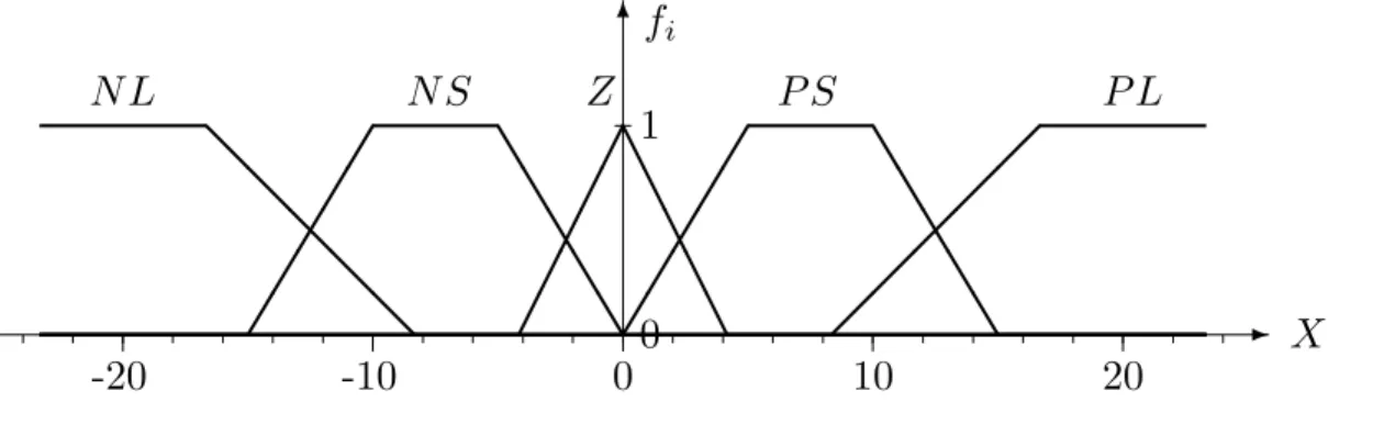
Figure 1: Fuzzy sets N L (negative large), N S (negative small), Z (zero), P S (positive small), and P L (positive large) covering the real line X = R.

The following two scalar characteristics of a fuzzy set will be useful later.

Definition: The weight w and the centroid c of a fuzzy set s = (X, f ) are defined as follows:

w = Z

f (x) dx and

c =

R xf (x) dx R f (x) dx

where all of the integrals are taken over the signal space X.

2 Fuzzification

Consider a signal space X covered by several fuzzy sets s _i , i = 1, . . . , k. The fuzzy question is: Given a vector x ∈ X, to which of the fuzzy sets s _i does x belong or, in which of the sets S i associated with the fuzzy sets s i does x lie?

In mathematical set theory, the answer for each of the sets S _i is a binary one. In fuzzy set theory, set membership is “by degree”.

Definition: Consider a fuzzy set s = (X, f ). An arbitrary element x ∈ X belongs to the fuzzy set s with degree d = f (x).

Hence, the answer to the fuzzy question is: x belongs to each of the fuzzy sets s i to some degree, viz., to degrees d i = f i (x), i = 1, . . . , k.

Examples: Consider the fuzzy sets N L, N S, Z , P S , and P L defined on the signal space X = R which are displayed in Figure 1.

a) The element x = − 20 is “negative large” to degree 1 and “negative small”,

“zero”, “positive small”, and “positive large” to degrees 0.

b) The element x = 2 is “negative large” and “negative small” to degrees 0,

“zero” to degree 0.52, “positive small” to degree 0.4, and “positive large” to degree 0.

3 Fuzzy Logic

Fuzzy logic defines the rules governing the operators intersection and union of fuzzy sets.

Consider two fuzzy sets s ₁ = (X, f ₁ ) and s ₂ = (X, f ₂ ) defined on the same signal space X and their associated sets S 1 ⊂ X and S 2 ⊂ X, respectively.

Definition: An arbitrary element x ∈ X belongs to the union s ₁ ∪ s ₂ of the two fuzzy sets s ₁ and s ₂ with degree d = max(f ₁ (x), f ₂ (x)).

Definition: An arbitrary element x ∈ X belongs to the intersection s ₁ ∩ s ₂ of the two fuzzy sets s ₁ and s ₂ with degree d = min(f ₁ (x), f ₂ (x)).

Consequently, the union operator and the intersection operator yield the fuzzy sets s ₁ ∪ s ₂ = (X, max(f ₁ , f ₂ )) and s ₁ ∩ s ₂ = (X, min(f ₁ , f ₂ )), respectively.

Notice that the intersection s ₁ ∩ s ₂ is a degenerated fuzzy set in the sense that

its set membership function min(f ₁ , f ₂ ) does not map onto the interval [0, 1] as

requested by the definition of a fuzzy set. This detail is not pursued any further

here because in fuzzy control, all calculations are done with fuzzy variables

rather than with fuzzy sets.

4 FUZZY VARIABLES 3

4 Fuzzy Variables

4.1 Introducing Fuzzy Variables

Definition: A fuzzy variable v is an ordered pair (s, d) where s is a fuzzy set and d ∈ [0, 1] a real bounded variable.

Fuzzy variables arise in the fuzzification operation in a natural way: For the variable x ∈ X , the real variable d is the degree of membership in the fuzzy set s. (Cf. Section 4.2)

In another interpretation of a fuzzy variable, the real variable d “modulates”

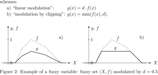
the fuzzy set s: The scalar d and the set membership function f : X → [0, 1] of the fuzzy set s define a new function g : X → [0, 1]. There are two modulation schemes:

a) “linear modulation”: g(x) = d · f (x) b) “modulation by clipping”: g(x) = min(f (x), d).

- -

6 6

1 1

0 0

g, f g, f

X X

f f

g g

a) b)

pp pp pp pp ppp p p p p p p p p p p p p p p p p pppp p pppp

p pppp p p pp pp pp pp ppp p p p p p p p p p p p p p p p p pppp

p pppp p pppp p p XXX

HH HH @

@@

Figure 2: Example of a fuzzy variable: fuzzy set (X, f ) modulated by d = 0.5:

a) linear modulation, b) modulation by clipping.

The author prefers the linear modulation scheme because the function g ob- tained by linear modulation typically contains more detailed information about the structure of the fuzzy variable.

In Section 1, the weight w and the centroid c of a fuzzy set s = (X, f ) have been defined. Obviously, the weight and the centroid of a fuzzy variable v can be defined in an analogous way by replacing the set membership function f by the modulated function g in these formulae.

Notice that the linear modulation scheme results in a linear reduction of the weight of the fuzzy variable, w _v = d · w _s , while the centroid remains unchanged, c _v ≡ c _s for all d ∈ (0, 1].

For calculations with a fuzzy variable, it is more practical to use the “mod-

ulated” function g than to keep the scalar d and the set membership function

f of the underlying fuzzy set s apart. Furthermore, the restriction g(x) ≤ 1 for

all x ∈ X can be dropped. This is practical when sums of fuzzy variables are

calculated.

4.2 Fuzzification Revised

Consider a signal space X covered by the N fuzzy sets s ₁ , . . . , s _N . An arbitrary element x ∈ X belongs to the fuzzy sets s 1 , s 2 , . . . , and s N to degrees d 1 = f 1 (x), d 2 = f 2 (x), . . . , and d N = f N (x), respectively.

Using fuzzy variables leads to the following definition of the fuzzification operation.

Definition: The fuzzification operator F maps an element x ∈ X to the set of fuzzy variables { (s ₁ , f ₁ (x)), (s ₂ , f ₂ (x)), . . . (s _N , f _N (x)) } .

Examples: Reconsider the examples a) and b) of Section 2. With the above definition we can rewrite the results succinctly in the following way:

a) F : − 20 7→ { (N L, 1), (N S, 0), (Z, 0), (P S, 0), (P L, 0) } and b) F : 2 7→ { (N L, 0), (N S, 0), (Z, 0.52), (P S, 0.4), (P L, 0) } .

4.3 Fuzzy Vectors

As the example in Section 4.2 shows, introducing vector notation in the range space of the fuzzification operator F is efficient.

Again, consider a signal space X covered by the N fuzzy sets s ₁ , . . . , s _N . The fuzzification F (x) of an arbitrary element x ∈ X can be represented by an N -vector in several equivalent ways:

F (x) =



 

 v ₁ v ₂ .. . v _N



 

 (x) =



 



(s ₁ , f ₁ (x)) (s ₂ , f ₂ (x))

.. . (s _N , f _N (x))



 

 ∼ =



 

 f ₁ (x) f ₂ (x)

.. . f _N (x)



 

 .

The relation operator “ ∼ =” points out the fact that, in the last vector, the fuzzy sets s i are not explicitly noted down but are implied by the indices i.

On the other side, every fuzzy n-vector can be represented by the corre- sponding modulated set membership functions g _i :



 

 v ₁ v ₂ .. . v _n



 

 =



 



(s ₁ , d ₁ ) (s ₂ , d ₂ )

.. . (s _n , d _n )



 

 =



 

 g ₁ g 2

.. . g n



 

 ∼ =



 



(w _g

, c _g

) (w g

, c g

)

.. . (w g

, c g

)



 

 .

Here, the relation operator “∼ =” points out the fact that the weight w _g

and the centroid c _g

do not completely characterize the fuzzy variable v _i .

This representation is useful at the outputs of the fuzzy rules describing a

fuzzy controller.

5 FUZZY RULES 5

5 Fuzzy Rules

Fuzzy rules are used in fuzzy control in order to define the map from the fuzzified input signals (error signals, measured signals, or command signals) of the fuzzy controller to its fuzzy output signals (control signals).

5.1 Fuzzy SISO-Rule

Consider a fuzzy set s _e = (E, f _e ) defined on the signal space E where the error signal e “lives” and a fuzzy set s u = (U, f u ) defined on the signal space U where the control signal u “lives”. (Usually, E = R and U = R, hence the designation

“SISO-rule”.)

Definition: The SISO-rule mapping the fuzzy input variable v _e = (s _e , d _e ) to the fuzzy output variable v _u = (s _u , d _u ) (of the fuzzy controller) is defined by v _u = (s _u , d _e ).

In the jargon of control engineering, this definition should be read as follows:

If the value e(t) of the error signal belongs to the fuzzy set s e to degree d e then the fuzzy set s _u of the control signal is fired to degree d _u = d _e , i.e., modulated by d _u = d _e .

In shorthand notation, the fuzzy SISO-rule is denoted by s _e ⇒ s _u , where the degree of firing d _u = d _e is implied.

The value u(t) of the control signal is obtained later by “defuzzification”

after all of the fuzzy rules pertaining to the control signal have been processed.

5.2 Fuzzy AND-Rules

Consider two fuzzy sets s _e1 = (E ₁ , f _e1 ) and s _e2 = (E ₂ , f _e2 ) defined on the signal spaces E ₁ and E ₂ , respectively, where the error signals e ₁ and e ₂ “live” and a fuzzy set s _u = (U, f _u ) defined on the signal space U where the control signal u

“lives”.

Definition: The AND-rule mapping the fuzzy input variables v e1 = (s e1 , d e1 ) and v _e2 = (s _e2 , d _e2 ) to the fuzzy output variable v _u = (s _u , d _u ) is defined by v _u = (s _u , min(d _e1 , d _e2 )).

In the jargon of control engineering, this definition should be read as follows:

If the value e ₁ (t) of the first error signal belongs to the fuzzy set s _e1 to degree d e

and the value e 2 (t) of the second error signal belongs to the fuzzy set s e2 to degree d e2 then the fuzzy set s u of the control signal is fired to the smaller of the two degrees, i.e., d _u = min(d _e1 , d _e2 ).

In shorthand notation, the fuzzy AND-rule is denoted by s e

∩ s e

⇒ s u ,

where the degree of firing d _u = min(d _e

, d _e

) is implied.

The value u(t) of the control signal is obtained later by “defuzzification”

after all of the fuzzy rules pertaining to the control signal have been processed.

It should be obvious how the definition of the fuzzy AND-rule can be ex- tended to three or more fuzzy input variables.

5.3 Other Fuzzy Rules

In analogy to the fuzzy AND-rules, fuzzy OR-rules or more complicated logical combinations for fuzzy rules could be defined.

The author prefers to use fuzzy AND-rules exclusively because OR-ing sev- eral AND-rules together typically results in a weaker contribution to the overall fuzzy output variable(s) and the corresponding defuzzified control variable(s).

Therefore, in the remainder of this report “fuzzy rule” stands for “fuzzy AND-rule” or its SISO special case “fuzzy SISO-rule”.

6 Fuzzy Associative Memory

For a fuzzy controller, the collection of all of its fuzzy rules is called the fuzzy associative memory.

For every control cycle, each of the fuzzy rules is evaluated. This can be done by massively parallel processing. The output of each fuzzy rule is a fuzzy variable.

The output of the fuzzy associative memory is equal to the (vector) sum of all these fuzzy variables:

In the case of a scalar control signal u(t), the signal space is the real line, U = R. Summing the fuzzy variables involves calculating the sum g u = P

j g j of their modulated functions g _j . — Notice that the fuzzy variable v _u at the output of the fuzzy associative memory is represented exclusively by the (“modulated”) function g _u . (I.e., this fuzzy variable has no directly underlying fuzzy set which is modulated by some degree d u to yield the function g u .)

In the case of a vector control signal u(t) ∈ R ^m , typically, the signal space of each of the components u _i (t) is the real line, i.e., U _i = R for i = 1, . . . , m.

Summing the fuzzy variables involves calculating the m sums g _u

= P

j g _ij of the modulated functions g ij for each index i, i = 1, . . . , m.

Of course, the summing operator P

takes the pointwise sum of its argument

functions. As mentioned in Section 4.1, the sum g(u) may execeed 1 for some

values of the argument u. This poses no problem (cf. Section 7). (Clipping g(u)

to the maximal value 1 would be counterproductive because the centroid of g

would be shifted.)

7 DEFUZZIFICATION 7

7 Defuzzification

Defuzzification is the process of assigning a representative value to a fuzzy vari- able. Consider a fuzzy variable v _u on the signal space U = R which is repre- sented by the modulated function g _u .

Definition: The defuzzification operator D maps the fuzzy variable v u to the centroid u of the modulated function g _u ,

u = D{ v u } = D{ g u } =

R αg _u (α) dα R g u (α) dα ,

where both of the integrals are calculated over the signal space U = R. The defuzzification operator D is understood to accept an arbitrary representation of the fuzzy variable v _u as its argument.

Upon conclusion of the fuzzy control algorithm, precise values u 1 (t), . . . , u m (t) must be assigned to the components of the control vector. However, the fuzzy associative memory yields m fuzzy variables v _u

(t) represented by their sum functions g _u

( · , t) = P

j g _ij ( · , t). Defuzzifying yields the control signals u i (t) = D{ v u

(t) } =

R βg _u

(β, t) dβ

R g u

(β, t) dβ i = 1, . . . , m

For the sake of simplicity, one-dimensional signal spaces U i = R for i = 1, . . . ,

m have been discussed. It would be rather straightforward to use signal spaces of

higher dimensions, in particular U = R ^m . The defuzzification of the m control

signals u _i (t) would then obviously involve the corresponding multiple integrals

over the signal space U = R ^m . — In practice, there is no advantage in using

such a generalization.

8 Fuzzy Control Systems

8.1 Structure of a Fuzzy Control System

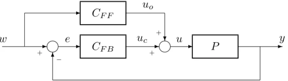
Sections 1, 2, and 4–7 describe all of the elements and operations needed in a fuzzy controller. Figure 3 shows the block diagram of a fuzzy control system implementing both feedback control and feed-forward control. All of the signals

- i - C F B - i - P - 6

C F F

-

?

w e u _c u y

u _o

+

−

+ +

Figure 3: Fuzzy control system consisting of the plant P , the fuzzy feedback controller C _{F B} , and the fuzzy feed-forward controller C _{F F} .

in Figure 3 are precise (i.e., crisp or non-fuzzy) signals. The internal structures of the feed-forward controller and the feedback controller are identical.

Figure 4 depicts the major components of the fuzzy feedback controller C _{F B} , viz., the fuzzifier F , the fuzzy associative memory F AM , and the defuzzifier D .

- F ≈≈≈≈ > F AM ∼∼∼∼∼ > D - e(t) v e (t) v u (t) u c (t)

Figure 4: Fuzzy feedback controller.

The “wiggly” or “fuzzy” double arrow emphasizes the fact that even for a scalar error signal e(t), the quantity v _e (t) = F{ e(t) } is a fuzzy vector (cf. Sections 4.2 and 4.3). On the other hand, v u (t) is a fuzzy variable which is defuzzified to the scalar control signal u c (t).

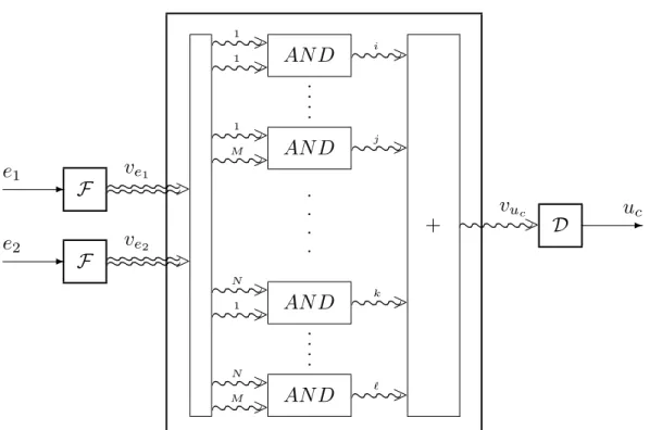
Figure 5 shows a detailed block diagram of a fuzzy controller with two input

signals and one output signal. The error signals e ₁ and e ₂ are fuzzified to the

fuzzy N -vector v _e

and the fuzzy M -vector v _e

, respectively. The components

of the fuzzy vectors, i.e., the N + M fuzzy variables are shipped to the N · M

fuzzy AND-rules. The fuzzy variables at the outputs of the AND-rules are

summed up. This yields the fuzzy control variable v _u

at the output of the

fuzzy associative memory and the defuzzified control signal u _c . — Notice that,

typically, one and the same fuzzy set of the control signal is fired by several of

the fuzzy AND-rules.

8 FUZZY CONTROL SYSTEMS 9

- F ≈≈≈≈≈≈ >

- F ≈≈≈≈≈≈ >

e 1 v e

e ₂ v _e

∼∼∼∼ >

∼∼∼∼ >

∼∼∼∼ >

AN D

∼∼∼∼ >

∼∼∼∼ >

∼∼∼∼ >

AN D pp pp

∼∼∼∼ >

∼∼∼∼ >

∼∼∼∼ >

AN D

∼∼∼∼ >

∼∼∼∼ >

∼∼∼∼ >

AN D pp pp

p p p p

+ ∼∼∼∼∼∼ v _u

> D - u c

1 1

1 M

N 1

N M

i

j

k

`

Figure 5: Detailed block diagram of a fuzzy feedback controller.

8.2 Example 1: Closed-loop halting control

In a fully automatic factory, parts, subassemblies, and the finished products are transported by several identical mobile robots. The navigation of the mobile robots about the factory is fully automated. In this example, the forward motion along the trajectories is considered only. Getting away from one station and cruising to the next station is under closed-loop speed control. The robot should stop at the next station within a very small tolerance for the position error.

Therefore, closed-loop halting control must be implemented.

The problem of designing a fuzzy control scheme for halting control is inves- tigated here.

The following information is available: The robot has a mass of anywhere between 150 and 450 kg, depending on the actual payload. The maximal cruising speed is 2 m/s. The positioning error at a station must be less than 1 mm. The maximal traction force for acceleration and deceleration is 500 N. The nominal deceleration in the approach to a station is a = 1 m/s ² . There is no requirement for the smoothness of the acceleration. At every station, within a reach of 2.5 m, a precise measurement of the instantaneous distance to the stop is transmitted to the robot at a very high rate. Furthermore, the robot has a precise velocity sensor.

The following concept for a fuzzy halting controller is chosen:

The control law for the forward motion of the robot is switched from cruise control to fuzzy halting control as soon as the simultaneous measurements p and v of the position and the velocity, respectively, satisfy the inequality

| p | ≤ v ² 2a .

At the switching time, a non-fuzzy signal generator for the setpoint variable w _p (t) for the position, the setpoint variable w _v (t) for the velocity, and the feed- forward force u _o (t) is initialized as follows:

w p (0) = p

w _v (0) = − sign(p) p 2a | p |

u o (0) = sign(p)m nom a = ± 250 N .

While the robot is in the halting control mode, the signal generator furnishes the setpoint values w _p (t) and w _v (t) and the feed-forward control signal u _o (t) according to the formulae

w _p (t) = w _p (0) + w _v (0)t + sign(w _p (0)) at ² 2 w _v (t) = w _v (0) + sign(w _p (0))at

u o (t) ≡ u o (0) ,

where t is the time elapsed since the initialization of the signal generator.

8 FUZZY CONTROL SYSTEMS 11

The error signals e _p (t) = w _p (t) − p(t) and e _v (t) = w _v (t) − v(t) are processed in a fuzzy feedback controller which produces the feedback force u c (t). The detailed block diagram of this fuzzy two-input one-output feedback controller corresponds to the one shown above in Figure 5. Finally, the total traction force is u(t) = sat { u _o (t) + u _c (t) } . (It is clipped to +500 N or − 500 N, respectively, whenever the sum exceeds the limit of the available traction force.)

The fuzzy halting control law is deactivated as soon as the velocity vanishes for the first time, v(t) = 0. Simultaneously, the parking brakes are set.

The fuzzy sets covering the signal space E _p = R where the position error e _p (t) lives are shown in Figure 6. The fuzzy sets covering the signal space E v = R where the velocity error e v (t) lives are shown in Figure 7.

- 6

1

0

-4 -2 0 2 4 [mm]

f _p

A p A A

A A P Z

@ @

@ @

@ P P S

P P L

@ @

@ @

@ P N S

HH HH

HH HH HH P N L

Figure 6: Fuzzy sets for the position error: P N L (negative large), P N S (nega- tive small), P Z (zero), P P S (positive small), and P P L (positive large).

- 6

1

0

-4 -2 0 2 4 [mm/s]

f v

v

@ @

@ @

@ V Z

@ @

@ @

@

V P S V P L

@ @

@ @

@ V N S

@ @

@ @

@ V N L

Figure 7: Fuzzy sets for the velocity error: V N L (negative large), V N S (nega- tive small), V Z (zero), V P S (positive small), and V P L (positive large).

The fuzzy sets chosen for the feedback traction force u c (t) are depicted in Figure 8. Notice that the centroids of the fuzzy sets U P X and U N X are located at − 500 N and +500 N, respectively, in order to give the fuzzy feedback controller full authority over the range − 500 . . . + 500 N. Furthermore, no fuzzy set U Z centered at 0 N is introduced in order to obtain “stiff” characteristics of the fuzzy feedback control law.

In Figure 9, the set of 20 fuzzy rules defining the fuzzy associative memory

of the fuzzy feedback controller is displayed. The entries of this tabloid should

- 6

1

0

-500 0 500 [N]

f _u

L u L L

L LL U P S

T T T

T T U P L

T T T

T T U P X

T T T

T T U N X

T T T

T T U N L

L L L

L LL U N S

Figure 8: Fuzzy sets for the control of the traction force: U N X (negative extra large), U N L (negative large), U N S (negative small), U P S (positive small), U P L (positive large), and U P X (positive extra large).

be read as explained in the following example. Shorthand explanation: P N L ∩ V N L ⇒ U N X . Longhand explanation: If e _p (t) belongs to the fuzzy set P N L to degree d ₁ and if e _v (t) belongs to the fuzzy set V N L to degree d ₂ then the fuzzy set U N X is fired to the smaller of the two degrees, i.e., to degree d = min(d ₁ , d ₂ ).

P N L P N S P Z P P S P P L v p : position error

V N L V N S V Z V P S V P L

v _v : velocity

error

U N X

U N X U N X U N L

U N L

U N L U N S

U N S

U N S

U N S U P S

U P S

U P S

U P S U P L

U P L

U P L U P X U P X

U P X

Figure 9: Fuzzy associative memory for the fuzzy closed-loop servo controller

containing twenty fuzzy rules.

8 FUZZY CONTROL SYSTEMS 13

In order to evaluate the effectiveness of the proposed fuzzy control scheme, the mobile robot is simulated. For the simulation, the “true” robot is modelled as follows:

˙

p(t) = v(t) p(0) = − 2 m

˙

v(t) = 1

m { u(t) − sign(v(t))γmg } v(0) = 2 m/s ,

where m = 150 . . . 450 kg is the true mass of the robot, g = 9.81 m/s ² the gravitational constant, and γ = 0.01 the coefficient of roll friction. For the simulations, digital control with a sampling and control rate of 500 Hz is as- sumed. This fairly high sampling rate is chosen in order to prevent mechanical resonances in the mobile robot.

In Figures 10 and 11, the trajectory of the robot is shown in the phase plane (p, v) in several scales for a true mass m = 450 kg and m = 150 kg, respectively.

For the complete trajectory labelled “a)”, the units for p and v are m and m/s, respectively. For the increasingly enlarged final parts “b)”, “c)”, and “d)” of the trajectory, the units are dm and dm/s, cm and cm/s, and mm and mm/s, respectively.

As the Figures show, the heaviest robot (m = 450 kg) overshoots the station by less than 0.2 mm, whereas the lightest robot (m = 150 kg) stops less than 0.2 mm short of the station. Hence, the specifications are met.

This servo control example is deceptively simple because the plant under con- sideration essentially is a double integrator and because with a PD-controller or with the equivalent linear state feedback controller one cannot arrive at an unstable control system, provided the signs of the two control gains are chosen correctly. The only open question is whether the specifications for the precision of halting are met.

From the next example it can be inferred that asymptotic stability of a

fuzzy control system is not necessarily obtained by choosing the fuzzy control

scheme with straightforward commonsense logic. As a matter of fact, proving

the asymptotic stability of a fuzzy control system (even of moderate complexity)

can turn out to be very difficult.

Figure 10: Trajectory of a robot with a mass of 450 kg in the phase plane (p, v).

Scales: a) m and m/s; b) dm and dm/s; c) cm and cm/s; d) mm and mm/s.

Figure 11: Trajectory of a robot with a mass of 150 kg in the phase plane (p, v).

Scales: a) m and m/s; b) dm and dm/s; c) cm and cm/s; d) mm and mm/s.

8 FUZZY CONTROL SYSTEMS 15

8.3 Example 2: Dog chasing cat

In this example, a dog chasing a cat is considered. Like most dogs, this dog is not smart enough to use proportional navigation. Rather, he tries to always run in the direction where he sees the cat. The dog would probably explain his scheme of navigation by the following qualitative rules for choosing the direction of his next leap: If the cat is straight ahead, I take the next leap in the same direction; if the cat is a little bit to the left (right), I turn a little bit to the left (right) for the next leap; if the cat is pretty much to the left (right), I turn quite a bit to the left (right) for the next leap.

Obviously, a fuzzy one-input one-output feedback controller for this scheme of navigation can be formulated with five fuzzy sets for the line of sight angle α(t k ), five fuzzy sets for the change of the dog’s heading angle ∆γ(t k ) for the next leap, and five fuzzy SISO-rules.

Figure 12 shows the fuzzy sets covering the signal space A = [ − 180 ^◦ , 180 ^◦ ] where the line of sight angle α(t _k ) lives. Figure 13 shows the fuzzy sets covering the signal space U = R where the change of the dog’s heading angle ∆γ(t k ) lives.

- 6

1

0

-180 ^◦ -45 ^◦ 0 ^◦ 45 ^◦ 180 ^◦

f _α

α A A A A AP S

AP L A A

A A AN L

A A A A AN S

B B B

B AZ

Figure 12: Fuzzy sets for the line of sight angle: AN L (negative large), AN S (negative small), AZ (zero), AP S (positive small), and AP L (positive large).

- 6

1

0

-180 ^◦ -90 ^◦ -45 ^◦ 0 ^◦ 45 ^◦ 90 ^◦ 180 ^◦

f _u

B ∆γ B B

B U P S

@ @

@ @ U P L

@ @

@ @ U N L

B B B

B U N S

B B B

B U Z

Figure 13: Fuzzy sets for the dog’s change of heading angle: U N L (negative large), U N S (negative small), U Z (zero), U P S (positive small), and U P L (pos- itive large).

The five fuzzy rules of the fuzzy associative memory of the fuzzy feedback

controller can be written in shorthand as follows: AN L ⇒ U N L, AN S ⇒ U N S,

AZ ⇒ U Z, AP S ⇒ U P S , and AP L ⇒ U P L. This should be read as follows:

If α(t k ) belongs to the fuzzy set AN L to degree d then the fuzzy set U N L for the change of heading angle should be fired to degree d, etc.

Since it is not quite clear what the dog means by “turning a little bit” or

“turning pretty much”, a multiplicative doggy gain K is introduced. Further- more, it is assumed that the dog cannot change his heading angle by more than 90 ^◦ in either direction from one step to the next. This leads to the final control law

u(t _k ) = ∆γ(t _k ) = sat { K D{ v _u (t _k ) }} ,

where v _u (t _k ) is the fuzzy variable at the output of the fuzzy associative memory at time t _k (cf. Figure 4).

In order to evaluate the effectiveness of the dog’s fuzzy feedback control, a

“dog chases cat” scenario is simulated.

In Figures 14 and 15, the cat runs along a rectangular course at constant speed, starting in the northwest corner. The dog starts running at a position close to the center of the rectangle. The dog’s speed exceeds the cat’s speed by 32.5 %. A blood stain is left on the ground whenever the dog intercepts the cat with very high precision but the chase continues immediately.

A natural value for the doggy gain is K = 0.5 since there is no reason why the dog should turn by more than 45 ^◦ when the cat is off by 45 ^◦ . The simulation for this value of the doggy gain is shown in Figure 14. Obviously, the dog performs reasonably well. Of course, whenever the dog overshoots the cat, he has to manoeuvre with a high turning rate until the cat is again “in front” of him.

In Figure 15, the simulation is done with K = 1. Now, the dog is zig-zagging most of the time, changing his direction by ± 90 ^◦ from step to step. He only catches the cat because he luckily happens to cut the southeast corner in an efficient way. Essentially, the dog fails his mission with this high value of the doggy gain. Note however, that the critical value for the doggy gain depends on how much the dog’s speed exceeds the cat’s speed.

In [9], the fuzzy pursuit problem of this example has been extended to a

fuzzy pursuit and evasion game, i.e., both the dog and the cat use fuzzy control

schemes.

8 FUZZY CONTROL SYSTEMS 17

Figure 14: The dog chases the cat with gain K = 0.5.

Figure 15: The dog chases the cat with gain K = 1.

9 Computational Issues

9.1 Efficient Defuzzification

Consider the task of simulating a fuzzy control system on a general purpose digital computer. For the simulation of the fuzzy (feedback) controller, Figures 4 and 5 suggest that the following sequence of operations should be executed at every sampling time:

• Fuzzify each of the error signals e _i to the corresponding fuzzy vector v _e

: v e

= F (e i ).

• Evaluate all of the fuzzy rules defined for the fuzzy controller. Each of the fuzzy rules yields a fuzzy variable v j which is represented by the modulated function g j (u).

• Calculate the sum of all of these fuzzy variables v j in order to get the fuzzy control variable v u = P

j v j which is represented by the function g(u) = P

j g _j (u).

• Defuzzify the fuzzy control variable v u by calculating its centroid u:

u = D (v _u ) =

R ug(u)du

R g(u)du .

Notice that for piecewise linear functions g _j (u), the sum g(u) is also a piece- wise linear function and both of the integrals of the defuzzification operation can be calculated analytically. Therefore, using fuzzy sets with piecewise linear set membership functions only (such as “triangles”, “trapezoids”, or piecewise lin- ear approximations of more sophisticated smooth functions) can lead to rather efficient program code.

In order to further reduce the run time of the simulation significantly, the result of the following lemma is needed.

Consider the modulated functions g _j , j = 1, . . . , N , and the corresponding function g = P N

j=1 g _j of the fuzzy control signal v _u . Let w _g

and c _g

be the weights and the centroids, respectively, of the modulated functions g _j , i.e.,

w _g

= Z

g _j (u) du and

c g

= Z

ug _j (u) du Z

g j (u) du

= 1 w g

Z

ug j (u) du .

9 COMPUTATIONAL ISSUES 19

Lemma: The defuzzified value u of the control variable can be obtained by evaluating the following purely algebraic equation:

u = D (v _u ) = X N j=1

w _g

c _g

X N j=1

w g

.

Proof:

u = D (v _u ) = Z

ug(u) du Z

g(u) du

= Z

u X N j=1

g j (u) du Z X ^N

j=1

g j (u) du

= X N j=1

Z

ug j (u) du X N

j=1

Z

g j (u) du

= X N j =1

w g

c g

X N j=1

w g

.

Notice that the weight w _g

and possibly the centroid c _g

vary as the degree d _j of firing for the corresponding fuzzy set s _j varies.

However, if the linear modulation scheme is used, the variable weights w g

and centroids c g

can be expressed by the constant weights w j and centroids c j

of the set membership functions f _j as follows:

w _g

= d _j w _j c _g

≡ c _j for j = 1, . . . , N . This observation leads to the following

Corollary: If the linear modulation scheme is used, the defuzzification opera- tion simplifies to

u = D (v _u ) = X N j=1

d j w j c j

X N j=1

d j w j

.

Of course, the N products w j c j need only be calculated once.

It now is obvious that in the Examples of Sections 8.2 and 8.3 there was

no need to fully specify the set membership functions of the fuzzy sets for the

control variables (cf. Figures 8 and 13, respectively). It would have sufficed to

merely specify their weights and their centroids. This could have been done in

the following equivalent way:

Example 1: Closed-loop halting control

fuzzy set s _i centroid c _i weight w _i

U N X − 500 N 277

U N L − 250 N 167

U N S − 100 N 111

U P S 100 N 111

U P L 250 N 167

U P X 500 N 277

Example 2: Dog chasing cat

fuzzy set s _i centroid c _i weight w _i

U N L − 90 ^◦ 9

U N S − 15 ^◦ 1

U Z 0 ^◦ 1

U P S 15 ^◦ 1

U P L 90 ^◦ 9

9.2 Derivatives of the Control Function

If the linear modulation scheme is used, the simplified defuzzification formula of the above Lemma lends itself to calculating derivatives of the control function in a straightforward way.

In order to keep the notation fairly simple, consider a fuzzy feedback con- troller with the p input signals e ₁ , . . . , e _p , the single output signal u, and N fuzzy AND-rules. The partial derivative ∂u/∂e i of the control function u(e 1 , . . . , e p ) with respect to the error signal e i is

∂u

∂e _i = Ã _N

X

j=1

∂d _j

∂e _i w j c j

!Ã _N X

j=1

d j w j

!

− Ã _N

X

j=1

d j w j c j

!Ã _N X

j=1

∂d _j

∂e _i w j

!

à _N X

j=1

d _j w _j

! 2 .

Notice that j numbers the fuzzy rules rather than the fuzzy sets defined for the control signal. One and the same fuzzy set of the control signal may be fired by more than one fuzzy rule (cf. Figure 9).

Discontinuities of these partial derivatives are caused both by the “corners”

of the (piecewise linear) set membership functions of the fuzzy sets covering

the signal spaces where e 1 , . . . , e p live and the “corners” of the functions

d _j = min( · · · ) of the fuzzy AND-rules.

9 COMPUTATIONAL ISSUES 21

9.3 Observations and Suggestions

For the sake of simplicity, consider a fuzzy SISO feedback controller. From the formulae for the defuzzification operator and for the derivative of the control function, the following observations and suggestions ensue:

• If none of the fuzzy sets of the control signal u is fired to a strictly positive degree, the value of the defuzzified control signal is undefined. Therefore, the signal space E , where the error signal e lives, must be covered com- pletely by its collection of fuzzy sets, and these fuzzy sets should overlap.

In other words, every error e ∈ E should belong to at least one fuzzy set to a strictly positive degree. Furthermore, in the associative memory, every fuzzy set of the error signal should fire (at least) one of the fuzzy sets of the control signal.

• If two neighbouring fuzzy sets of the error signal “touch” at e ₁ but do not overlap, the control function is discontinuous at e ₁ . For e = e ₁ , the result of the defuzzification operator is undefined. The value of the control signal must be defined separately. — In Example 1 (fuzzy halting control), the analogous situation occurs for e _p = e _v = 0. The obvious extra definition is u _c (0, 0) = 0.

• Assume that the linear modulation scheme is applied. If in some interval [e _a , e _b ] ⊂ E the error e belongs to exactly one fuzzy set to a strictly positive degree, the control function is constant on this interval, irrespective of the shape of this fuzzy set for the error signal. — In Example 2 (dog chasing cat), the dog will turn by ∆γ = sat { K · 15 ^◦ } if the line of sight angle α is in the interval [15 ^◦ , 22.5 ^◦ ], or by ∆γ = sat { K · 90 ^◦ } if the line of sight angle exceeds 45 ^◦ . (Obviously, the dog could improve his performance significantly by choosing the centroids +45 ^◦ and − 45 ^◦ for the fuzzy sets U P L and U N L, respectively, and the doggy gain K = 1.)

• Assume that the linear modulation scheme is applied. For the purpose of implementing a finished design of a fuzzy controller, only the weights w _i and the centroids c i of the fuzzy sets for the control signals are needed in the defuzzification operation (cf. Section 9.1). — On the other hand, the complete specifications of the set membership functions of the fuzzy sets for the control signals are needed, if the fuzzy rules of the controller must be “learnt” by watching an expert performing the task at hand. This topic is beyond the scope of this report. The interested reader is referred to [1], and [8], and the references cited there.

• In Section 8, “static” fuzzy controllers are considered only. The reader

should have no problem in extending these ideas to fuzzy controllers incor-

porating “dynamic compensation”. In the simplest case the input signals

of the fuzzy dynamic compensator include the most recent error signals

e _i (k) and the delayed error signals e _i (k − 1), e _i (k − 2), etc., and perhaps previously issued control signals u j (k − 1), u j (k − 2) etc.. In the latter case it is efficient to refuzzify the defuzzified control signals in order to obtain the required delayed fuzzy control variables. All or most of the processing is performed in the fuzzy part of the controller. In more sophisticated cases, non-fuzzy dynamic compensation (e.g., in the form of a full state observer) can be performed in a preprocessor to the fuzzy controller proper.

References

[1] B. Kosko, Neural Networks and Fuzzy Systems: A Dynamical Systems Ap- proach to Machine Intelligence, Prentice-Hall, Englewood Cliffs, NJ, USA, 1992.

[2] H.-J. Zimmermann, Fuzzy Set Theory and its Applications, 2nd ed., Kluwer, Boston, MA, USA, 1991.

[3] W. Pedrycz, Fuzzy Control and Fuzzy Systems, Electronic & Electrical En- gineering Research Studies, Control Theory and Applications Series, vol. 3, Research Studies Press (Wiley), Taunton, Somerset, England, 1989.

[4] D. J. Dubois, H. M. Prade, Fuzzy Sets and Systems, Academic Press, New York, NY, 1980.

[5] L. A. Zadeh, Fuzzy Sets and Applications: Selected Papers, Wiley-Inter- science, New York, NY, USA, 1987.

[6] M. M. Gupta, T. Yamakawa, (eds.), Fuzzy Computing, Hardware, and Ap- plications, North-Holland, Amsterdam, Netherlands, 1988.

[7] M. Sugeno, (ed.), Industrial Applications of Fuzzy Control, North-Holland, Amsterdam, Netherlands, 1985.

[8] C.-T. Lin, C. S. G. Lee, “Neural-Network-Based Fuzzy Logic Control and Decision Systems,” IEEE Transactions on Computers, vol. 40(1991), pp. 1320–1336.

[9] S. Ginsburg, R. Wimmer, H. P. Geering, “Clever Dog versus Smart Cat,”

Proceedings of the International ICSC Symposium on Fuzzy Logic, pp. A99–

A104, Zurich, Switzerland, May, 1995.

[10] H. Kiendl, Fuzzy Control methodenorientiert, Oldenbourg, Munich, Ger-

many, 1997.