On Classical and Quantum Mechanical Energy Spectra of Finite Heisenberg Spin Systems

(1)

On Classical and Quantum Mechanical Energy Spectra of Finite Heisenberg Spin Systems

Dissertation

zur Erlangung des Grades eines Doktors der Naturwissenschaften

Dem Fachbereich Physik vorgelegt von

Dipl.-Phys. Matthias Exler

Osnabr¨ uck, M¨ arz 2006

(2)

(3)

Betreuer und Erstgutachter : Apl. Prof. Dr. J. Schnack Zweitgutachter : Jun.-Prof. Dr. J. Gemmer

Datum der m¨undlichen Pr¨ufung: 8.Mai 2006

(4)

(5)

List of Figures

2.1 Internal energy for the spin ring N = 6, s= ⁵₂ . . . 10

2.2 Specific heat for the spin ring N = 6,s= ⁵₂ . . . 11

2.3 High-temperature approximation of the specific heat . . . 12

2.4 Lowest energy eigenvalues of {Mo₇₂Fe₃₀} (DMRG results) . . . 16

2.5 Rotational band energy levels in{Mo₇₂Fe₃₀} . . . 20

2.6 Broadened rotational band model for {Mo72Fe30} . . . 22

2.7 Allowed INS transitions in the rotational band model . . . 32

2.8 Dependence of INS energy transfer on magnetic field . . . 34

2.9 Relative height of INS peaks depending on magnetic field . . . 35

2.10 Inelastic neutron scattering on{Mo₇₂Fe₃₀} at T = 65mK,B = 0 . . . 37

2.11 INS spectrum of{Mo₇₂Fe₃₀}for different temperatures at B = 0 . . . 39

2.12 Simulated INS spectrum of{Mo₇₂Fe₃₀}forB = 0 . . . 39

2.13 INS spectrum of{Mo₇₂Fe₃₀}forB 6= 0 . . . 40

2.14 Simulated INS spectrum of{Mo₇₂Fe₃₀}forB 6= 0 . . . 41

3.1 Classical density of states for the spin ring with N = 6 . . . 52

3.2 Classical density of states for the spin trimer . . . 53

3.3 Convergence of the classical density of states . . . 54

3.4 Classical MC results for the specific heat . . . 59

3.5 Wang-Landau sampling: density of states of the trimer . . . 66

3.6 Wang-Landau sampling: density of states of the ring with N = 6 . . . 66

3.7 Wang-Landau sampling: density of states of {Mo₇₂Fe₃₀} . . . 67

4.1 Spectra of spin-coherent states for the ring with N = 6, s= ⁵₂ . . . 78

4.2 Spectra of spin-coherent states for the ring with N = 10, s= 1 . . . . 78

4.3 Comparison of broadening functions with given second moment . . . . 86

4.4 Distribution of uncertainty for the ringN = 6,s= ⁵₂ . . . 87

4.5 Classical and corrected spectrum for the ring with N = 6,s= ⁵₂ . . . 87

4.6 Quantum corrected specific heat of the ring withN = 6,s= ⁵₂ . . . . 88

4.7 Distribution ofσ(E) for different spin quantum numbers . . . 90

4.8 Classical spectrum of the ring with N = 6, s= ⁵₂ . . . 91

4.9 Specific heat of the ring N = 6,s= ⁵₂ from cut classical spectrum . . . 92

4.10 Specific heat of different systems from cut classical spectrum . . . 93

(8)

(9)

1 Introduction

Polyoxometalate chemistry has successfully improved the synthesis of magnetic molecules in recent years. Since the synthesis of Mn₁₂ [1], which can be regarded as the birth of this new class of materials, many different molecules of various sizes and structures have been produced [2, 3]. These molecules consist of many atoms, but their magnetic nature originates from a number of paramagnetic ions, whose unpaired electrons form collective angular momenta, referred to as spins. The number of interacting spins ranges from as few as two up to several dozens, which is realized in the giant Keplerate molecule {Mo72Fe30}, where 30 paramagnetic Fe³⁺ ions occupy the vertices of an icosidodecahedron [4].

Magnetic molecules usually appear as macroscopic samples. However, the magnetic interactions between molecules are often negligible compared to the intramolecular interactions. Measurements of the sample hence reflect properties of single molecules, which are significantly different from bulk magnets. Various possible fields of application may be offered by the magnetic molecules, including quantum computing, data storage, nano switches, and even biomedicine [2, 3, 5, 6]. However, some applications have to be considered as speculative so far. Our main interest in magnetic molecules arises from the fact that they represent mesoscopic quantum systems, i.e. they can neither be described as single particles nor as solids.

In most magnetic molecules the localized spins couple antiferromagnetically, and the interaction can be accurately described by the Heisenberg model [7]. For the under- standing and prediction of the properties of a spin system, the eigenvalue spectrum of the Hamiltonian has to be calculated or at least approximated. To this end, various methods have been developed, or adopted from other fields.

The existence of symmetries can allow the analytical solution of the eigenvalue problem. Analytical solutions are found very rarely, since their derivations often rely on special substitutions of the operators in the Hamiltonian, which are possible only for certain systems. Furthermore, no general recipe can be given for the development of an analytical solution. The existence (and knowledge) of an analytical solution hence remains an exceptional situation. However, analytical solutions are extremely valuable for the verification of numerical data, so that new algorithms can first be applied to systems whose eigenspectra are known, and used to calculate data for other systems only after they have been proven to deliver accurate results.

Another more general tool for the calculation of the eigenvalue spectrum is the numerical exact diagonalization method. It is not limited to a special class of systems,

(10)

but only by the size of the Hilbert space of the model. The term “numerical exact method” refers to the fact that the method uses the unmodified Hamiltonian, hence it is exact, but incorporates numerical algorithms to perform the diagonalization.

This approach is therefore only exact with respect to the numerical precision of the algorithm and the computer it is processed on. Exact diagonalization is limited to small systems, since the size of the Hilbert space grows exponentially with the number of spins, although the exploitation of symmetries can help to reduce the effective size [8].

For the analysis of ground state (or low-temperature) properties, the Lanczos or DMRG methods [9] extend the class of numerically treatable molecules, since they reduce the numerical effort by targeting only a limited number of eigenstates.

Monte Carlo methods have been utilized to calculate thermodynamic properties directly, but their main focus is on the behavior of an infinite lattice of spins [10].

Although the simulations are performed with a finite number of spins, the results are extrapolated after analyzing the dependence on the system size. The application of Monte Carlo methods to magnetic molecules is only found rarely, e.g. in references [11, 12].

The methods presented above operate on the unmodified Hamiltonian, the approximation arises from the use of numerical algorithms with a limited precision or the reduction of the set of solutions. Another approach of approximation is the substitu- tion of the Hamiltonian by a simplified model that can be diagonalized more easily.

The Ising model, e.g., reduces an s= ¹₂ Heisenberg system to a dependence on only the z-component, and the Ising Hamiltonian is automatically diagonal in the basis of ˆS^z-eigenstates. Analytical solutions are known for both one- and two-dimensional Ising systems, hence the Ising model has become the standard model to demonstrate and verify Monte Carlo implementations [10].

For the class of magnetic molecules, the rotational band model was introduced to describe the low-energy spectrum of the antiferromagnetic Heisenberg Hamiltonian [13]. Whereas some structures (e.g. dimer, trimer, tetrahedron) possess strict rotational bands, the spectra of ring systems and various polytopes were shown to exhibit a nearly quadratic dependence on the total spinS.

In this work, we will use the rotational band model to derive an approximation of the inelastic neutron scattering (INS) cross-section of {Mo₇₂Fe₃₀} (see chapter 2). We will analyze the degeneracies of the eigenvalues and infer the dependence of the energy spectrum on an external magnetic field. Our results are then compared to INS experiments, which were performed at various temperatures and magnetic field strengths. The verification of our results by comparison with the experiment is intended to broaden the knowledge of the range of applicability of the rotational band model. The model has already been shown to comply with magnetization and susceptibility data [14], but since inelastic neutron scattering can directly measure the excitation spectrum of the molecule, the successful application of our approach

(11)

substantiates the validity of the rotational band model.

Whereas the comparison of the rotational band model approximation to experimental results verifies a theory that was developed specifically for magnetic molecules, this class of materials can serve as an example for studying general questions of quantum mechanics, as well.

Since chemistry now allows the preparation of magnetic molecules with various spin quantum numbers, this class of materials can also be utilized for studying the relations between classical and quantum regime. Due to the correspondence principle, a quantum spin system can be described exactly by classical physics for s → ∞. However, the question remains for which quantum numberss a classical calculation yields a reasonable approximation. Classical Monte Carlo has been used to study the properties of several magnetic systems [10], and the numerical data has been successfully verified by experiments. The general assumption is that, for high temperatures, the classical model can accurately predict the thermodynamic properties, and that with growing spin quantum number, the range of applicability extends to lower temperatures, since the system approaches the classical limit.

However, the argument for the allowed temperature range, where the quantum system essentially behaves as a classical system, is often derived from the comparison with the experiment, rather than from the analysis of the quantum Hamiltonian.

Our approach in this work is to develop a converging scheme that adds systematic quantum corrections to the classical density of states. To this end, we will first introduce the classical density of states in chapter 3 by giving a general definition and relating it to statistical thermodynamics. We will give an exact solution for Heisenberg spin rings, derived from an expression for the partition function. Fur- thermore, we will discuss the two stochastic algorithms of classical Monte Carlo and Wang-Landau sampling. Whereas Monte Carlo is mainly used as a reference method for thermodynamic quantities, Wang-Landau sampling is able to give a numerical approximation of the density of states itself.

The classical density of states is determined by the phase space volume of an energy shell, i.e. all phase space points whose corresponding energies lie within a given energy interval. The definition of the quantum spectrum is rather different, since it is derived from the discrete set of energy eigenvalues [15]. Nevertheless, we will implement a formalism that connects quantum and classical spectrum. The correspondence of the two differently defined quantities relies on special quantum states that span the Hilbert space and are parametrized by continuous variables. The main requirement for these states is, however, that the expectation value of the quantum Hamiltonian equals the value of the classical Hamiltonian function for the given parameters. For the Heisenberg model this correspondence is satisfied by the spin-coherent states.

The main goal of the work presented in chapters 3 and 4 is to derive a controllable, converging algorithm that approximates the quantum spectrum of a general Heisen- berg spin system. The availability of such a method is eminently valuable, since

(12)

other approaches such as classical Monte Carlo rely on empirical arguments whether the system is in the classical domain or not. Furthermore, our algorithm allows the analysis of how the classical limit is approached, which gives general criteria for the similarity of the classical density of states to the quantum spectrum.

(13)

2 Quantum mechanical eigenvalue spectrum

This chapter deals with aspects of the quantum mechanical energy spectrum of spin systems. We will first introduce the Heisenberg Hamiltonian, which is used throughout this thesis. The spectrum is then related to thermodynamical properties of the system. The main focus of the chapter is on approximate methods to describe the spectrum. After reviewing the eigenvalue problem and discussing aspects of exact diagonalization, we will give brief summaries of two simplifications of the spectrum.

The rotational band model is presented more thoroughly, since it will be used to explain results of neutron scattering experiments later.

2.1 Heisenberg model

In the work presented here, we will solely use the Heisenberg model to describe magnetic interactions between the localized magnetic moments of the molecules. The Heisenberg model introduces an effective Hamiltonian, describing the electrostatic interactions between the electrons as a coupling of the spins of the ions. The magnetic exchange interactions between two spins of the system are assumed to be scalar products of the spin angular momentum operators, multiplied by the exchange parameter J:

Hˆ₁₂=Jˆs₁·ˆs₂ . (2.1) For a magnetic molecule, the Heisenberg Hamiltonian for the whole system is written as the sum over all interacting pairs,

Hˆ =X

i<j

J_ijˆs_i·ˆs_j , (2.2)

where J_ij denotes the interaction matrix, containing the exchange parameters of pairs (i, j). The sign of the exchange parameter determines the type of interaction, i.e. J_ij >0 denotes antiferromagnetic exchange, and J_ij < 0 denotes ferromagnetic exchange. This is easily deduced from eq.(2.2), when the spin operators are replaced by classical vectors. Positive J then favors anti-parallel alignment of the vectors.

(14)

2.1.1 Angular momentum operators

The operators ˆs_i in eq.(2.2) are spin angular momentum operators. We will give a brief summary of their properties [16].

The states |si are eigenstates of the square of the spin operator ˆs:

ˆ

s²|si=s(s+ 1)|si (2.3)

The components of the vector operator ˆs satisfy the commutation relation hˆs^α,ˆs^βi

= iǫ_αβγˆs^γ with α, β, γ ∈ {x, y, z}, (2.4) whereǫ_αβγ denotes the Levi-Civita symbol. All components commute with the square of the spin operator:

ˆs²,sˆ^α

= 0 with α∈ {x, y, z}. (2.5) However, the components do not commute with each other, and the usual choice for the axis of quantization is thez-axis. We can form a basis of the Hilbert space with eigenstates of the ˆs^z-operator, denoted by |s, mi:

ˆ

s^z|s, mi=m|s, mi. (2.6)

The quantum numbermcan take valuesm=−s,−s+ 1, . . . , s(the dimension of the Hilbert space is 2s+ 1), and the states are connected with the ladder operators

ˆ

s⁺|s, mi=p

s(s+ 1)−m(m+ 1) |s, m+ 1i (2.7) and

ˆ

s⁻|s, mi= ˆs⁺†

|s, mi=p

s(s+ 1)−m(m−1) |s, m−1i (2.8) The ladder operators can be expressed as linear combinations of the x- and y- components of ˆs:

ˆ

s⁺= ˆs^x+ iˆs^y and sˆ⁻= ˆs^x−iˆs^y , (2.9) Note that we have set the Planck constant ~= 1 in all definitions. This convention is used throughout this thesis, unless we specifically require~, e.g. for the derivation of the classical limit of a quantum mechanical property.

Product states

For a system ofN spins, the Hilbert space is the product of the single-spin Hilbert spaces. The basis states can be expressed as product states

|s₁, m₁, s₂, m₂, . . . , s_N, m_Ni:= |s₁, m₁i ⊗ |s₂, m₂i ⊗ · · · ⊗ |s_N, m_Ni. (2.10)

(15)

2.1 Heisenberg model

The dimension of the product Hilbert space is dimH=

YN i=1

(2s_i+ 1), (2.11)

or in case of a common spin quantum numbers,

dimH= (2s+ 1)^N . (2.12)

The total spin operator of the system is the sum of the individual spin operators:

Sˆ= XN i=1

ˆ

s_i . (2.13)

However, the product states of the form (2.10) are not eigenstates of ˆS², but of the z-component of the total spin

Sˆ^z = XN

i=1

ˆ

s^z_i , (2.14)

with

Sˆ^z|s₁, m₁, s₂, m₂, . . . , s_N, m_Ni

= Xn i=1

m_i

!

|s₁, m₁, s₂, m₂, . . . , s_N, m_Ni, (2.15) wherePn

i=1m_i is referred to as the quantum numberM. 2.1.2 Magnetic field

Eq.(2.2) only describes the mutual interactions of the spins of the molecule. Being magnetic moments, the spins naturally interact with an external field, as well. The Zeeman Hamiltonian describes the interaction of a magnetic moment with an external magnetic fieldB:

Hˆ_Zeeman=−gµ_BB·Sˆ , (2.16)

where the magnetic moment is proportional to the total spin ˆS of the system with the Land´e factor g = 2 and the Bohr magneton µ_B. Since we assume the isotropic Heisenberg model, we can choose thez-axis as the axis of quantization, and the total Hamiltonian can be written as

Hˆ =X

i<j

Jijˆs_i·ˆs_j−gµBBSˆ^z, (2.17) where B is the magnetic field in z-direction. Note that the sign of the Zeeman interaction is arbitrary, since the Heisenberg model is symmetric in changing the sign of the total quantum number M. We have chosen the minus sign for compatibility with previous numerical calculations.

(16)

2.2 Exact diagonalization

The basis for the calculation of any physical property of the system is given by the eigensystem of the Hamiltonian. In order to obtain the eigenvalues and eigenstates, the equation

Hˆ|ψi=λ|ψi (2.18)

has to be solved.

For the numerical evaluation of the eigensystem, the Hamiltonian has to be expressed by its matrix representation H, i.e. H_ij = hi|Hˆ |ji, where the states |ii with i= 1,2, . . . ,dimHform a basis of the Hilbert space. The algorithm then uses matrix operations to find the matrix U that diagonalizes the Hamiltonian H:

H_diag=U^†HU (2.19)

The columns of the matrix U represent the eigenvectors, and H_diag is a diagonal matrix containing the eigenvalues (hence the term “diagonalization”). The numerical exact diagonalization results presented here are calculated using the linear algebra package LAPACK [17].

Since the diagonalization is an algorithm that scales with the cube of the dimension of the Hilbert space, it is important to minimize this dimension. If one can find a set of mutually commuting operators, the diagonalization can be performed in subspaces characterized by the quantum numbers related to the chosen operators. For the Heisenberg Hamiltonian, e.g., one can use the total ˆS^z-operator with the corresponding quantum numberM to divide the Hilbert space into mutually orthogonal subspacesH(M), and perform the diagonalization in each subspace separately. In the case of a ring system, a “shift-operator” T can be defined, which cyclically remaps each spin to its next neighbor position. It commutes with both ˆH and ˆS^z and can be used to further reduce the dimensions of the matrices to be diagonalized. For molecules of different structures, analogous symmetry operators can often be found.

2.2.1 Thermodynamic averages

The statistical operator describing the canonical ensemble is given by [18]

ˆ

ρ= e^−β^H^ˆ

Tre^−β^H^ˆ , (2.20)

where the denominator is referred to as the partition function:

Z(β) = Tre^−β^H^ˆ =X

ν

e^−βE^ν , (2.21)

withβ = 1/k_BT and E_ν the eigenvalues of ˆH.

(17)

2.3 Approximation of the quantum mechanical energy spectrum

Thermodynamic averages are evaluated using the trace over the product of the statistical operator and the respective observable ˆA:

hhAˆii= Tr ˆ ρAˆ

= 1 Z Tr

e^−β^H^ˆAˆ

. (2.22)

The internal energy is defined as the thermodynamic mean of the Hamiltonian of the system:

U(β) :=hhHˆii= 1 Z(β)

X

ν

E_νe^−βE^ν =− ∂

∂β lnZ(β). (2.23) The specific heat can either be expressed as a second order derivative of the partition function, or it can be described by the fluctuations of the Hamiltonian:

C(β) = ∂U

∂T

V

=kBβ² ∂²

∂β² lnZ(β) (2.24)

=kBβ²

hhHˆ²ii − hhHˆii²

. (2.25)

2.3 Approximation of the quantum mechanical energy spectrum

After discussing the exact diagonalization of the Hamiltonian in the previous section, we will now give examples of approximations of the energy spectrum. These methods will not be used to derive new results, but they will serve as background for discussions in later sections. Although the rotational band model described in section 2.4 certainly is a method for the approximation of the quantum mechanical energy spectrum, it is presented in a separate chapter, since it will be used to explain experimental results in section 2.5

2.3.1 ”Binning” of energy eigenvalues

The true spectrum of a Heisenberg system consists of a vast number of different eigenvalues (up to dimH, if no degeneracies are present). We will now analyze the effect of reducing the number of distinct contributions to the spectrum by summating over the weights of the eigenvalues contained in equally-sized energy intervals (energy bins). The resulting approximated spectrum then consists only of the central energies of the bins and the corresponding summated weights.

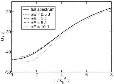
Figure 2.1 shows the temperature dependence of the internal energy with applied

“binning” of the spectrum compared to the exact result. The approximations with

∆E≤5J can accurately describe the exact dependence except for very low temperatures. Since the curves are qualitatively very similar, the internal energy does not

(18)

0 2 4 6 8 T / k_B^-1 J

-50 -40 -30 -20

U / J

full spectrum

∆E = 0.5 J

∆E = 1 J

∆E = 5 J

∆E = 10 J

Figure 2.1:Internal energy vs. temperature for the spin ring with N = 6, s = ⁵₂. The solid line represents the result for the full eigenvalue spectrum; other curves are approximations for “binned” spectra with the given width of the energy bins.

provide us with an adequate tool for the distinction of the quality of the approximations.

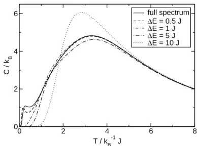
Figure 2.2 shows the specific heat for different widths of the energy bins. The main features of the exact curve are reproduced by all “binned” spectra but the ones with

∆E ≥5J, which significantly differs for the temperature interval that is shown. The other two curves can reproduce the exact one for almost all temperatures. Only forJ⁻¹k_BT <1, we can see a deviation from the so-called “Schottky peak”¹ which is determined by the gap between ground state and first excited state (E₁ −E₀ ≈ 0.692J). This energy difference cannot be reproduced by a binned spectrum with equidistant intervals, unless the width of the bins equals this energy gap (or is a divisor, respectively).

Comparing to the results for the internal energy, we find that the specific heat is more sensitive to the level of approximation of the energy spectrum. It exhibits much stronger visual differentiation between the curves, since it is a second-order derivative of the partition function, whereas the internal energy is of first order. We will therefore use the specific heat as the measure of quality for other approximate methods described in later sections.

1The Schottky peak is referred to as the maximum of the specific heatC(T) of a system with two energy levels

(19)

2.3 Approximation of the quantum mechanical energy spectrum

0 2 4 6 8

T / k

B -1 J 0

2 4 6

C / k B

full spectrum

∆E = 0.5 J

∆E = 1 J

∆E = 5 J

∆E = 10 J

Figure 2.2:Specific heat vs. temperature for the spin ring with N = 6, s = ⁵2. The solid line represents the result for the full eigenvalue spectrum; other curves are approximations for “binned” spectra with the given width of the energy bins.

2.3.2 High-temperature expansion of the partition function

The partition function (2.21) can be expressed as a series of traces of powers of ˆH:

Z = Tre−βHˆ = X∞ n=0

(−1)ⁿ

n! βⁿTr ˆHⁿ. (2.26) This can be used to derive a high-temperature (low β) expansion of the internal energy, since the literature lists exact expressions for traces of powers of ˆH [19]:

Tr ˆH⁰ = (2s+ 1)^N = dimH, (2.27)

Tr ˆH¹ = 0, (2.28)

Tr ˆH² = X

i<j

J_ij²1

3s²(s+ 1)²(2s+ 1)^N . (2.29) Inserting (2.26) into the definition (2.23) and keeping only first-order terms inβ, one obtains

U(β)≈ −Tr ˆH²

Tr ˆH⁰ β . (2.30)

Hence, the high-temperature limit of the specific heat can be expressed as C(T) = Tr ˆH²

Tr ˆH⁰ 1

k_BT² , (2.31)

(20)

which becomes

C(T) = N

3s²(s+ 1)² 1

kBT² (2.32)

for rings withN sites.

The high-temperature limit is equivalently obtained when the energy spectrum is approximated by a Gaussian distribution with the same variance as the Hamiltonian H.ˆ

-40 -20 0 20 40

E / J 0

0.01 0.02 0.03 0.04

g(E)

q.m. spec.

Gaussian

0 5 10 15 20

T / k_B^-1 J 0

2 4 6 8 10

C / k B

exact q.m.

Gaussian

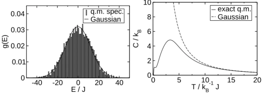
Figure 2.3:Spin ring withN = 6,s=⁵2. Left: histogram of the quantum mechanical energy spectrum (width of bins ∆E= 1J) and approximation with a Gaussian. Right:

high-temperature approximation of the specific heat compared to exact quantum mechanical result.

Figure 2.3(left) shows a histogram of the quantum mechanical eigenvalue spectrum of the spin ring with N = 6, s = ⁵₂. The general shape of the energy distribution is well described by the Gaussian, which has the same variance as the Hamiltonian.

The histogram entries add up to a total weight of 1, and the normalization of the Gaussian is chosen so that it matches the histogram.

The graph on the right of figure 2.3 gives a comparison of the high-temperature approximation of the specific heat with the exact result. Since only the second moment of the energy distribution is used, we could not expect any details of the shape of the specific heat to be reproduced by this approximation.

Classical limit of the variance of Hˆ

As mentioned in section 2.1.1, we set ~= 1 in all equation, unless otherwise noted.

When we rewrite eq.(2.29) with ~, we can calculate the classical limit of the width of the spectrum. The classical limit is approached when~→0 and s→ ∞, so that

~s→1. For the variance of the spectrum, this means that

slim→∞

~→0

Tr ˆH²

Tr ˆH⁰ = lim_s_→∞

~→0

1 3

X

i<j

J_ij²

~⁴s²(s+ 1)² = 1 3

X

i<j

J_ij²

. (2.33)

(21)

2.4 Rotational band model

The above formula allows us to calculate the variance of the classical density of states analytically, thus providing a tool for the verification of numerical Wang-Landau results (cf. Sec. 3.5).

2.4 Rotational band model

The thermodynamic behavior of a quantum system can be described completely, if the full energy spectrum is known. However, the full quantum spectrum is not always accessible. In the case of spin systems, the dimension of the Hilbert space grows exponentially with the number of spins.

On the other hand, the Boltzmann factor e⁻^k^Ei^B^T decides how much a given energy eigenstate state |ψ_iicontributes to the thermodynamic averages. If the temperature is low, only a small number of energy levels is actually occupied and a huge part of the spectrum can be neglected. It is therefore still valuable to develop an approximation that can only describe the low-energy part of the spectrum.

For magnetic molecules of the form of rings with an even number of spins, it was found that the series of minimum energies in subspaces of the total spinH(S) follow a Land´e rule: (E_min(S)−E₀)∝S(S+ 1) [20, 21].

These systems are bipartite, i.e. they can be decomposed into two sublattices of spins, with no spin interacting with any other spin of the same sublattice. Classical systems of this kind have a well known ground state referred to as a N´eel state. Neighboring spins are aligned anti-parallelly (next-nearest neighbors are parallel). This feature of the classical ground state can be used to construct a quantum mechanical trial state as an approximation of the true ground state. The N´eel-like quantum ground state would consist of two spins SA and SB, representing each sublattice and assuming their maximum value S_A = S_B = ^{N s}₂ , which are coupled to a total spin of S = 0.

The series of all N´eel-like quantum states from coupling to the minimum S = 0 to the maximumS =N sleads to a parabolic energy spectrum [22]:

E_N´_eel(S) = 4 J 2N

S(S+ 1)−2N s 2

N s 2 + 1

(2.34) The factor 4 fixes the equality of the energy of the N´eel-like state withS =N sand the ground state of the corresponding ferromagnetically coupled system, which has E = JN s². The term rotational band was introduced for this type of spectrum, because it resembles the spectrum of a rigid rotor.

Eq.(2.34) describes the spectrum of a two-spin system with an interaction strength of ^2J_N, where both spins ˆS_A and ˆS_B have quantum numbers S_A= S_B = ^{N s}₂ . Thus, an equivalent representation of (2.34) can be given by an effective Hamiltonian [13]

Hˆ = 4 J 2N

hSˆ²−Sˆ²_A−Sˆ²_Bi

. (2.35)

(22)

The above equation can be used to derive an approximation of the whole spectrum, because the spins of the sublatticesA and B can be allowed to couple to sublattice spin values between S_A = 0 and S_A = ^{N s}₂ (S_B accordingly). Reference [13] shows that many systems exhibit a second parabolic band above the lowest one (N´eel band).

In the rotational band model, this first excited band can be described by coupling the two sublattice spins with S_A = ^{N s}₂ (maximum) and S_B = ^{N s}₂ −1 (maximum decreased by one) to a total spin S = [1,2, . . . , N s−1]. The missing S = 0 level also agrees with the exact spectra of bipartite systems. However, higher excitations should not be expected to be described adequately by the rotational band model.

In reference [13] it was also shown that the rotational band model can be extended to rings with an odd number of spins as well as to other structures like octahedra, icosahedra, and rings with next-nearest neighbor interaction. The formula for the series of minimum energy states in subspacesH(S) has to be modified to match the given structure:

E_min(S)≈E₀+JD(N, s)

2N S(S+ 1). (2.36)

The spin- and size-dependent parameter D(N, s) describes the curvature of the parabola, whereas E₀ is the ground state energy. These parameters were adjusted so that eq.(2.36) reproduces the ground state energies of both the antiferromagnetic and the ferromagnetic case. It was found that eq.(2.36) then showed good numerical agreement to the minimum energies of the H(S) subspaces of the full Heisenberg Hamiltonian.

2.4.1 Application to {Mo₇₂Fe₃₀}

Since the number of states in {Mo₇₂Fe₃₀} is astronomically large ((2s+ 1)^N = 6³⁰, which is about Avogadro’s number), we don’t have access to the true energy spectrum of this molecule. However, we can establish an approximation of the spectrum using the rotational band model described in the previous section.

The ground state of the corresponding classical Hamiltonian of {Mo₇₂Fe₃₀}, where the vector spin operators are replaced by classical vectors, can be found analytically.

Using graph theory, one can show that the corresponding graph to the interaction matrixJij in eq.(2.2) is three-colorable. This means each site can be assigned one out of three colors, so that none of the neighboring sites has the same color. Therefore, the ground state structure is composed of three sublattices, each containing ten spins.

On each of these sublattices, all spins point to the same direction. The sublattice vectors are coplanar, and the angle between each two of them is 120 degrees [23].

The knowledge of the classical ground state forms the basis for the construction of an approximate quantum Hamiltonian according to the rotational band model. The ten spins on each sublattice first couple to a super-spin, and these three spin operators

(23)

Sˆ₁, ˆS₂, and ˆS₃ then interact via a Heisenberg Hamiltonian:

Hˆ_rot.band=JD(N, s) N

hSˆ₁·Sˆ₂+ ˆS₂·Sˆ₃+ ˆS₃·Sˆ₁i

=JD(N, s) 2N

hSˆ²−Sˆ²₁+ ˆS²₂+ ˆS²₃i

. (2.37)

In order to achieve a better approximation of the real spectrum in the form of eq.(2.36), the refined Hamiltonian introduced in reference [24] is used. A parameter γ is introduced, which adjusts the offset determined by the configuration of the sublattice spins, and thereby shifts the ground state energy.

Hˆ_rot.band =JD(N, s) 2N

hSˆ²−γ

Sˆ²₁+ ˆS²₂+ ˆS²₃i

. (2.38)

This Hamiltonian can easily be diagonalized, and its energy eigenvalues are E(S;S₁, S₂, S₃) =JD(N, s)

2N

"

S(S+ 1)−γ X3 k=1

S_k(S_k+ 1)

#

. (2.39)

This follows from the fact that each sublattice spin operator ˆS_k commutes with the total spin ˆS² and both the other sublattice spins.

Using the simple model, we can generate an approximate energy spectrum for our molecule. We can independently choose the three sublattice spins in the allowed interval

0,^N₃s= 25

. We refer to a band as the series of energy levelsE(S;S₁, S₂, S₃) we get for a given choice ofS₁,S₂, andS₃, when the total spin quantum number S is varied. The energy levels of the lowest band are obtained when all sublattice spin quantum numbers assume their maximum value,S_k= ^N₃s= 25.

The parameters D(N, s) and γ can be derived by enforcing the same energy eigenvalue of the ferromagnetic ground state for both the full Heisenberg Hamiltonian and the simplified rotational band model. The ferromagnetic ground state exhibits the maximum total spinS=N s, and the corresponding energy eigenvalue is

E = 2N s²J = 60 (5

2)²J = 375J (2.40)

for the full Hamiltonian (2.2). The energy is doubled compared to a ring system of N spins because each spin in{Mo72Fe30} has four instead of two neighbors. In the simple model, the parameterγ = 1. Hence, the parameterDhas to equal 6, in order eq.(2.39) yieldsE = 2JN s² forS =N sandS_k= ^{N s}₃ (all sublattice spinsS_k assume their maxima and couple to the maximum total spin).

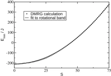
In earlier investigations [25], we have confirmed that the series of lowest energies of the H(S) subspaces indeed show a nearly parabolic dependence on S. Figure 2.4

(24)

shows our numerical results for the eigenvalues of the full Heisenberg Hamiltonian using the DMRG algorithm [9, 26], and a fit to the refined rotational band model as in eq.(2.39). The least-squares fitting procedure yields parameters D= 6.17 and γ = 1.05, leading to a good global consistency of both curves.

0 25 50 75

S -200

-100 0 100 200 300 400

E min / J

DMRG calculation fit to rotational band

Figure 2.4:DMRG approximations for the lowest energy eigenvalues in subspacesH(S), and the corresponding fit to the rotational band model

An alternative method to determine the parameters is by comparing to magnetization measurements, resulting inD= 6.23 andγ = 1.07 [24]. The good agreement with the above mentioned values ofD= 6 andγ= 1 shows the applicability of this simplified model.

Magnetic field

Adding a Zeeman term (cf. Sec. 2.1.2) for the interaction with a magnetic field, eq.(2.38) becomes

Hˆ_rot.band =JD(N, s)

2N Sˆ²−γ X3 k=1

Sˆ²_k

!

−gµBBSˆ^z . (2.41) Therefore the energy levels are:

E(S, M) =JD(N, s) 2N

"

S(S+ 1)−γ X3 k=1

S_k(S_k+ 1)

#

−gµ_BBM . (2.42)

(25)

Sources for degeneracies of energy levels

Each band generated by eq.(2.36) consists only of S_max+ 1 = S₁ +S₂ +S₃ + 1 different energy levels (S = [0,1, . . . , S_max]). However, the dimension of the Hilbert space (2s+ 1)^N = 6³⁰ is retained by the simplified Hamiltonian, and these bands are highly degenerate. The sources for the degeneracies can be classified by four types:

Type a): Coupling paths of sublattice spins

There are different paths to couple the ten spins to the respective sublattice spinS_k. The number of degeneracies can be calculated using the following procedure:

Starting with one spin of quantum numberS₁ =s(where the index 1 now denotes the number of spinsN, and not the number of the sublattice), the possible total spin when coupled to another spin of the same kind can beS₂ = [|S₁−s|= 0,1, . . . , S₁+s= 2s].

There is only one path to reach each of the possible values ofS₂. When another spins is added, the total spinS₃ of three spins can assume values from 0 (¹₂ for half-integer s) to 3s. Now for each possible configuration ofS3, one has to add the degeneracies of all thoseS₂ configurations that can be coupled with sto the resulting S₃. Coupling S₂ withsto S₃ is possible, if

|S₂−s| ≤S₃ ≤S₂+s . (2.43) The procedure is continued accordingly until the total number of spins is reached (S₁₀ in the case of the {Mo₇₂Fe₃₀}sublattices).

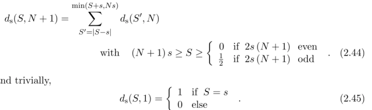
Another formulation of the above can be given with a recurrence formula. The number of paths leading to a given configuration (S, N) is

d_s(S, N + 1) =

min(S+s,N s)

X

S^′=|S−s|

d_s(S^′, N)

with (N + 1)s≥S ≥

0 if 2s(N + 1) even

1

2 if 2s(N + 1) odd . (2.44) and trivially,

ds(S,1) =

1 if S=s

0 else . (2.45)

Table 2.1 illustrates the algorithm for the example of coupling four spins s= ³₂. In order to find the number of paths leading to S₄ = 2, the degeneracy levels of the three-spin system have to be summed fromS₃ =|S₄−s|= ¹₂ to S₃ =S₄+s= ⁷₂. Accordingly, the coupling paths for the sublattice spins (ten spinss= ⁵₂) were calculated using a simple computer program implementing eq.(2.44). Table 2.2 only shows the numbers of coupling paths which are interesting for our simulation, since

(26)

S

N 0 ¹₂ 1 ³₂ 2 ⁵₂ 3 ⁷₂ 4 ⁹₂ . . .

1 1

2 1 1 1 1

3 2 4 3 2 1 . . .

| {z }

4 11

...

Table 2.1: Coupling pyramid for ans= ³₂ system

only the sublattice spin configurations with largeS_kare responsible for the low-lying rotational bands.

S

N 0 ¹₂ 1 ³₂ 2 ⁵₂ 3 ⁷₂ 4 ⁹₂ 5 . . . 23 ⁴⁷₂ 24 ⁴⁹₂ 25

1 1

2 1 1 1 1 1 1

3 2 4 6 5 4 . . .

...

10 . . . 45 9 1

Table 2.2: Coupling pyramid for a sublattice spin of the rotational band model. Ten spins withs= ⁵₂ are coupled to the resulting sublattice spin.

Type b): Permutation of lattice spins

The three sublattice spins S_k contribute symmetrically to the Hamiltonian (2.38).

They can therefore be permuted without changing the energy eigenvalue. The number of permutations depends on the configuration of the sublattice spinsS_k:

d_perm(S₁, S₂, S₃) =







1 ifS1 =S2 =S3 3!

2! = 3 if only two of theS_k are equal 3! = 6 if the S_k are all different

. (2.46)

Type c): Coupling paths for total spin

A given set of sublattice spinsS₁,S₂ and S₃ can be coupled to the total spin S via different paths. The procedure to calculate the number of these paths is similar to the

(27)

one described for type a). Whereas for type a) ten spins of the same quantum number s= ⁵₂ were coupled, theS_k can assume different values in the interval

0,^{N s}₃ = 25 . Since we have already calculated the number of permutations of the lattices, we can now choose one sequence for the coupling. At first, S₁ and S₂ are coupled to S₁₂, then the third sublattice spin S3 is added to S12 to obtain the total spinS.

The simple algorithm was implemented using a loop counting from S₁₂ =|S₁−S₂| toS₁₂=S₁+S₂. For everyS₁₂that satisfies the condition|S₁₂−S₃| ≤S ≤S₁₂+S₃, the counter d_S(S₁, S₂, S₃) is incremented.

Type d): M-degeneracy

In case of no applied magnetic field, the Hamiltonian (2.41) is independent of ˆS^z. Therefore, each energy level is dM = 2S + 1 times degenerate (quantum number M can assume values from −S to +S). This degeneracy is of course lifted when a magnetic field is present.

Product of degeneracies

Thus, the degeneracy for a given eigenstate of the rotational band Hamiltonian, characterized by the total and the three sublattice spin quantum numbers, is given by the product of all types of degeneracies introduced above:

d(S, S₁, S₂, S₃) =d_s(S₁)·d_s(S₂)·d_s(S₃) (type a)

·d_perm(S₁, S₂, S₃) (type b)

·d_S(S₁, S₂, S₃) (type c)

·d_M(S) (type d) (2.47)

2.4.2 Energy levels and degeneracies of the lowest two bands

The lowest band is formed by coupling the sublattices with equal (maximum) spin S₁ =S₂ =S₃= 25. Therefore, the degeneracy of these energy levels arises only from types c) and d) of the above mentioned sources. The level of degeneracy according to type c) can be calculated using the inequality |S12−S3| ≤ S ≤ |S12+S3|, with S₃ = 25 and 0 ≤ S₁₂ ≤ 50. Depending on S, there are two situations. When S≤25, the right inequality always holds, and only|S₁₂−25|needs to be evaluated.

All configurations S12={25−S,25−S+ 1, . . . ,25 +S} can couple to the given S, leading to a (2S+ 1)-fold degeneracy.

In the case ofS >25, the left inequality is always satisfied. Therefore, onlyS₁₂+25≤ S is to be considered, yielding S₁₂={S−25, S−25 + 1, . . . ,50}.

(28)

The ˆS^zdegeneracy type d) is always (2S+1)-fold. This leads to the following formula:

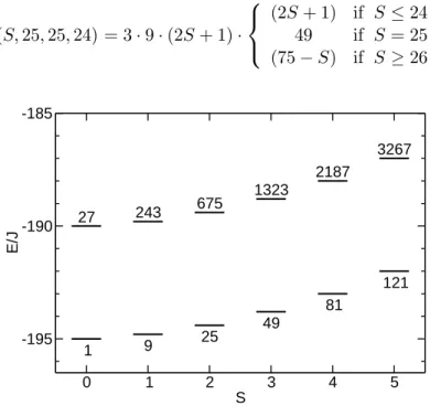
d(S,25,25,25) = (2S+ 1)·

(2S+ 1) if S≤25

(76−S) else . (2.48) The levels of degeneracy in the first excited band (S₁ =S₂ = 25, S₃= 24) also have a component of type a) and type b). In the coupling pyramid for ten spins s = ⁵₂ (table 2.2), we find nine paths to couple ten spins with s = ⁵₂ to a total S = 24.

There are three permutations of the lattice spinsS₁,S₂,S₃ in this case. The level of degeneracy of type c) can be calculated analogously to the lowest band:

d(S,25,25,24) = 3·9·(2S+ 1)·







(2S+ 1) if S ≤24 49 if S = 25 (75−S) if S ≥26

. (2.49)

1 9 25 49

81

121

27 243 675 1323

2187

3267

0 1 2 3 4 5

S -195

-190 -185

E/J

Figure 2.5:Rotational band model for {Mo⁷²Fe³⁰}. Numbers next to the energy levels specify the level of degeneracy, with none of the types of degeneracies lifted mentioned in section 2.4.1

Figure 2.5 illustrates the energy levels and the degeneracies for the lowest two bands for small S. The two bands are parallel and are separated by an energy gap of E¹(S)−E⁰(S) = 5γJ withγ = 1 for this graph.

2.4.3 Field dependence of the ground state

When the external magnetic fieldB is raised, the Zeeman energy in eq.(2.42) lifts the (2S+ 1)-fold degeneracies of the ˆS²-eigenstates. Due to the linearity of the Zeeman

(29)

energy with the M quantum number, states from multiplets with higher S become ground state with increasing magnetic field.

One can calculate the total spin of the ground state depending on the external magnetic fieldB. According to eq.(2.42), the minimum energy states (M =S) have

E(S) =JD(N, s) 2N

"

S(S+ 1)−γ

nL

X

k=1

S_k(S_k+ 1)

#

−gµBBS . (2.50) Introducing the dimensionless variables

B^′ = 2N gµ_B

DJ B , E^′ = 2N

DJE , (2.51)

eq.(2.50) simplifies to

E^′(S) =S(S+ 1)−B^′S−const. (2.52) The energy difference between two levels E^′(S) and E^′(S+ 1) in the same band is

E^′(S+ 1)−E^′(S) = 2(S+ 1)−B^′, (2.53) and therefore, these levels cross at magnetic field strengths of

B_cross^′ = 2(S+ 1). (2.54)

Thus, the spin quantum number of the ground state at the current magnetic field is the largest integer smaller than B^′/2:

S₀(B^′) = B^′

2

. (2.55)

2.4.4 Lifting of degeneracies

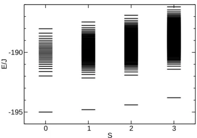
Due to its simplicity, the rotational band model possesses certain characteristics that are absent for the exact Hamiltonian (2.2). The degeneracies introduced by the simplified Hamiltonian (2.38) are likely to be lifted in this complex structure, i.e. energy levels in this system are presumably not exactly aligned to parabolic bands. Therefore, one might think of the following change to the model. Instead of assuming all levels exactly at the calculated band energy E(S, S₁, S₂, S₃), one could rather group the levels around those energies, with eq.(2.39) only describing the average energy in the respective band.

This broadening of the bands could be described by Gaussian distributions of energy levels centered at the respective band energy. The density of states can then be expressed as

ρ(E)∝e−^[E−E(S,S_2σ¹²^,S²^,S³^)]² . (2.56)

(30)

0 1 2 3 S

-195 -190

E/J

Figure 2.6:Energy levels for{Mo⁷²Fe³⁰}with broadened rotational bands. The degeneracies of figure 2.5 are all lifted except for type d) (M-degeneracy). The broadening parameter is σ= 1J.

The Gaussian has a mean value of E(S, S1, S2, S3) and its variance is specified by σ². A distribution with the required Gaussian density can be generated by inverting the integral of the density ρ(E) and applying the resulting function to a uniform distribution [27].

E = Φ⁻¹(x) =√

2σerf⁻¹(1−2x) with x∈(0,1) (2.57) yields a Gaussian distribution for the energy E with varianceσ². For an improvement of our approximation, we can now generate energy levels with a broadening parameter σ_band using the above formula:

E_j(S) =E(S, S₁, S₂, S₃) − σ_band σ(n_S)erf⁻¹

1−2 j n_S+ 1

; j = 1,2, . . . , n_S. (2.58) erf⁻¹ denotes the inverse error function, and n_S is the degeneracy of the respective energy level, excluding the degeneracy arising from theM quantum number:

n_S =d_s(S₁)·d_s(S₂)·d_s(S₃)·d_perm(S₁, S₂, S₃)·d_S(S₁, S₂, S₃). (2.59) Eq.(2.57) is strictly valid only for continuous distributions. The variance of a discrete set generated with this formula differs from the desiredσ² (in the limit of largenthis difference vanishes). In order to obtain a distribution of energy levels with variance

(31)

2.5 Inelastic neutron scattering on{Mo₇₂Fe₃₀}

σ_band, the fraction _σ(n^σ^band

S) is introduced to formula (2.58) with σ²(n_S) = var

erf⁻¹

1−2 j n_S+ 1

j=1,2,...,nS

(2.60) being then_S-dependent variance of the generator.

Figure 2.6 shows an example spectrum with broadened bands (broadening parameter σ= 1J). The band structure is still visible since the density of states is concentrated at the band energies of eq.(2.39), however, the spectrum could be more realistic than the pure rotational band structure with its artificial degeneracies.

2.5 Inelastic neutron scattering on { Mo

₇₂

Fe

₃₀

}

This chapter deals with the simulation of inelastic neutron scattering (INS) spectra for {Mo₇₂Fe₃₀} using the rotational band model. A brief introduction on neutron scattering will be given, both on principal experimental setup and on basic theory.

Thereafter, we will outline the relations between properties of the magnetic probe and the cross-section of the scattering process. We will recall the information on the energy spectrum of {Mo₇₂Fe₃₀}developed in the previous chapter. The insights gained from the above will then be used to derive a simple method to simulate INS spectra for{Mo₇₂Fe₃₀}for given temperatures and external magnetic field strengths.

This simulation is then compared to experimental results, and the quality of our method is discussed with respect to these results.

2.5.1 Introduction

Neutrons are baryons and form the basis of atomic nuclei together with the protons.

They carry no charge, but a spin of s_n = ¹₂, their mass is m_n = 1.008665 u. The operator of the magnetic moment for a neutron is

ˆ

µ_n= γ_nµ_Nσˆ (2.61)

withµ_N= _2m^e^~

p ≈5.050·10⁻²⁷J T⁻¹being the nuclear magneton andγ_n =−1.91 the gyromagnetic ratio for neutrons. The operator ˆσ represents the Pauli spin matrices.

According to their kinetic energy, neutrons are classified into groups relating the energy to a temperature scale. The INS experiments on{Mo72Fe30}were carried out using cold neutrons (E ≈ 2 meV ≈ 20k_BK), i.e. with a substantially lower energy compared to thermal neutrons (k_B·300 K≈25 meV).

Neutrons can be obtained from nuclear reactions such as take place in accelerator collisions or nuclear reactors. Since they have no charge, neutrons cannot be as easily directed or accelerated as protons or electrons.

(32)

At the ISIS pulsed neutron source [28], a high-energy beam of protons is directed to a metal target, where the collision process creates neutrons that are emitted in all directions. To achieve coherentk-vectors for the scattering experiments, the actual facilities for performing INS experiments are supplied with neutrons via long tubes emerging from the spallation target area.

The interaction between neutrons and matter is relatively weak, and the penetration depth in matter is very large, making neutrons suitable mainly for analyzing bulk properties. Neutron scattering can measure the undistorted properties of the target sample, manifested in the fact the cross-section can be written as a product of two parts, a response function depending only on the target sample, and a function describing the neutron-matter interaction (cf. Sec. 2.5.2). INS experiments are therefore an excellent tool to investigate the nature of the energy spectrum of magnetic molecules.

The basic quantity measured in an INS experiment is the partial differential cross- section

dσ²

dΩ dE^′ . (2.62)

Given an incident beam of neutron of energyE, it denotes the fraction of neutrons scattered into the element of solid angle dΩ around Ω with energies betweenE^′ and E^′+ dE^′. In the following paragraph, we will give a short outline of scattering theory necessary to calculate the cross-section from properties of the target material. We mainly reproduce the derivation given in reference [29]:

2.5.2 Outline of scattering theory

At first, an expression for the cross-section of elastic scattering is developed. An incident neutron, described by a plane wave function ψ_k = ¹

L^3/2 e^ik·r, is scattered into the plane wave functionψk^′. The probability of state ψkchanging toψk^′ can be calculated using Fermi’s Golden rule:

W_k→k^′ = 2π

~ Z

drψ_k^∗^′V ψˆ _k

2

ρ_k^′(E). (2.63)

Vˆ denotes the interaction potential of the neutron with the target, and ρ_k^′(E) the density of final scattering states per energy unit. This result is derived from perturba- tion theory and is therefore only approximate. However, the scattering of neutrons at the target is a weak process, justifying the assumption the scattering can be described perturbatively.

Enclosing the entire system into an artificial box of volumeL³, normalizing the states ψ_k and ψ_k^′, and relating the incident flux of neutrons to their velocity, the cross-