1
Shape matters: the relationship between cell geometry and diversity
1
in phytoplankton.
2
Alexey Ryabov1,2*, Onur Kerimoglu1,3, Elena Litchman4, Irina Olenina5,6, Leonilde Roselli7, Alberto 3
Basset8,9, Elena Stanca8, and Bernd Blasius1,2 4
5
Affiliations:
6
1Institute for Chemistry and Biology of the Marine Environment, University of Oldenburg, Oldenburg, 7
Germany 8
2Helmholtz Institute for Functional Marine Biodiversity (HIFMB), Carl von Ossietzky University 9
Oldenburg, Oldenburg, Germany 10
3Insistute of Coastal Research, Helmholtz-Zentrum Geesthacht, Geesthacht, Germany 11
4W. K. Kellogg Biological Station, Michigan State University, Hickory Corners, MI 49060, USA 12
5Environmental Protection Agency, Klaipėda, Lithuania 13
6Marine Research Institute of the Klaipeda University, Klaipėda, Lithuania 14
7Agency for the Environmental Prevention and Protection (ARPA Puglia), Lecce, Italy 15
8Department of Biological and Environmental Science and Technologies, University of Salento, Lecce, 16
Italy 17
9Institute of Research on Terrestrial Ecosystems, National Research Council, Lecce Italy 18
*Correspondence to: alexey.ryabov@uni-oldenburg.de.
19 20
2 21
Summary
22
Organisms’ size and shape profoundly influence their ecophysiological performance and 23
evolutionary fitness, suggesting a link between morphology and diversity. We analyse global 24
datasets of unicellular phytoplankton, major group of photosynthetic microbes with an 25
astounding diversity of cell sizes and shapes, and explore the distribution of taxonomic diversity 26
across different cell shapes and sizes. We find that cells of intermediate volume have the greatest 27
shape variation, from oblate to extremely elongated forms, while small and large cells are mostly 28
compact (e.g., spherical or cubic). Taxonomic diversity varies across cell elongation and cell 29
volume, with both traits explaining up to 92% of its variance. It decays exponentially with cell 30
elongation and displays a log-normal dependence on cell volume, peaking for compact, 31
intermediate-volume cells. Our findings point to the presence of different selective pressures and 32
constraints on the geometry of phytoplankton cells and, thus, improve our understanding of the 33
evolutionary rules of life.
34
Phytoplankton are major aquatic primary producers that form the base of most marine food webs 35
and are vital to the functioning of marine ecosystems. Marine unicellular phytoplankton exhibit an 36
enormous diversity (Hutchinson, 1961), with cell volumes spanning many orders of magnitude and 37
dozens of different shape types, from simple spherical to extremely complex cells (Reynolds, 2006).
38
This huge variation in phytoplankton cell volumes and shapes presents a unique opportunity for 39
investigating evolutionary constraints on morphological traits and their connection to taxonomic 40
richness, because the geometry of a phytoplankton cell plays an important role in its adaptation to 41
the environment. Cell size and shape affect most aspects of phytoplankton survival, from grazing by 42
zooplankton (Pančić and Kiørboe, 2018; Sunda and Hardison, 2010) to sinking (Durante et al., 2019) 43
and diffusion (Padisák et al., 2003), diffusive transport limitation (Kiørboe, 2008) and nutrient uptake 44
(Edwards et al., 2012; Grover, 1989; Karp-Boss and Boss, 2016; Tambi et al., 2009). While the role of 45
cell size in determining phytoplankton fitness and diversity has been documented previously 46
(Cermeño and Figueiras, 2008; Ignatiades, 2017), not much is known about the role of cell shapes.
47
Here, we characterize broad patterns in cell shapes and their relationship with cell volume and 48
taxonomic richness across main phyla of unicellular marine phytoplankton and heterotrophic 49
dinoflagellates (together called below, for brevity, phytoplankton). We compiled one of the most 50
comprehensive data sets of phytoplankton in terms of sizes, shapes and taxonomic diversity from 51
seven globally distributed marine areas: North Atlantic (Scotland), Mediterranean Sea (Greece and 52
Turkey), Indo-Pacific (the Maldives), South-western Atlantic (Australia), Southern Atlantic (Brazil) and 53
Baltic Sea (see Methods). The data comprises 5,743 cells of unicellular phytoplankton from 402 54
genera belonging to 16 phyla. We classified each cell as one of 38 fundamental geometric shapes, 55
such as spheres, cylinders, prisms, etc., measured cell linear dimensions and calculated the surface 56
area and volume for each cell (Hillebrand et al., 1999; Olenina et al., 2006; Vadrucci et al., 2007) (see 57
Methods). Cell volumes span almost 10 orders of magnitude, from 0.065 𝜇m3 for the 58
cyanobacterium Merismopedia to 5 ∙ 108 𝜇m3 for Dinophyceae’s Noctiluca.
59
The degree of shape elongation can be expressed as the aspect ratio and surface relative extension 60
(see Methods). The aspect ratio, 𝑟, characterizes the linear dimension of cell elongation, and is less 61
than one for oblate (flattened at the poles) shapes, and is greater than 1 for prolate (stretched) 62
shapes. We also define a shape as compact if 2/3 < 𝑟 < 3/2. The surface extension, 𝜖, shows the 63
relative gain in surface area of a cell compared to a sphere with the same volume. The minimum 64
level of surface extension is shape-specific and equals 1 for spheres, 1.14 for cylinders, 1.24 for 65
3
cubes, and 1.09 for double cones (see Methods). The two measures of shape elongation are related, 66
and the logarithm of the aspect ratio changes approximately with the square root of surface 67
extension (Extended Data Fig. 2).
68
Variation in cell shape
69
We found that the taxonomic diversity across different phyla varies with cell shape type and 70
elongation (Fig. 1A). Most Bacillariophyta (diatoms) are cylindrical or prismatic, while other phyla are 71
mostly ellipsoidal, with additional shapes, e.g., conic or of a more complex geometry, being relatively 72
rare. In our database, 46% of genera are prolate, 38% compact and only 16% oblate (Fig. 1B). These 73
proportions vary across phyla and shapes (Extended Data Fig. 1). For instance, more than half of 74
genera classified as elliptical cells have a compact shape, while for other shapes more than half of 75
genera have prolate cells. Oblate shapes comprise up to 20% of genera in diatoms, dinoflagellates 76
(Miozoa), Haptophyta, Charophyta, Cryptophyta, and Euglenozoa, but are rarer (< 10%) in other 77
phyla. Half-shapes such as half-spheres or half-cones are more dominated by oblate forms.
78
Shape elongation is hypothesized to influence phytoplankton fitness. Several studies argued that 79
elongation is beneficial for the volume-specific nutrient uptake and, therefore, large cells should be 80
elongated to increase the surface to volume ratio (Lewis, 1976; Niklas, 2000). However, our analysis, 81
based on the order of magnitude more cell measurements than in previous studies (Lewis, 1976;
82
Niklas, 2000), shows that cell surface area increases with volume approximately to the power of 2/3 83
(Fig. 2A), indicating that cell dimensions scale on average isometrically with volume, and there is no 84
evidence for more shape elongation with increasing volume.
85
By contrast, the variation in cell elongation strongly depends on cell volume (Fig. 2C, Extended Data 86
Fig. 3). The distribution of the surface extension as a function of cell volume is approximately hump- 87
shaped, with a peak of cell elongation at intermediate volumes (between 103− 104 𝜇𝑚3), where 88
the cell surface area can exceed the surface area of a sphere with an equivalent volume up to 5-fold.
89
In contrast, for cells of very small or large volume, surface extension approaches its minimum values, 90
implying that these cells have a compact shape minimizing their surface area. The hump-shaped 91
pattern is also seen in the 75% and 90% quantiles (Fig. 2C), confirming that this is not a sample 92
artifact. The same pattern emerges for the aspect ratio, which reaches 100 for prolate cells and 93
drops to 0.025 for oblate cells (Extended Data Fig. 3). This pattern also holds across different trophic 94
guilds (autotrophic, mixotrophic or heterotrophic); however, the maximum cell elongation is 95
reached only by the autotrophs, while in heterotrophs and mixotrophs the maximum aspect ratio 96
equals 10 and the maximum surface extension equals 2 (Extended Data Fig. 4), likely because these 97
two groups need to swim actively.
98
Phytoplankton diversity distribution
99
Taxonomic diversity, 𝐷, measured here as richness of genera, depends on both cell volume and 100
surface extension. It follows a lognormal function of volume with a peak of diversity at 𝑉0= 1100 ± 101
90 𝜇𝑚3 (Fig. 2D, 𝑅𝑎𝑑𝑗2 = 0.98) and decreases exponentially with shape surface extension 𝜖 as 102
𝐷~𝑒−1.43𝜖 (Fig. 2E, 𝑅𝑎𝑑𝑗2 = 0.97). Both relationships vary across cell shapes (Extended Data Fig. 5, 103
6). The ellipsoidal cells have the diversity distribution peaking at the smallest volume, compared to 104
other shapes (𝑉0= 330 ± 40 𝜇𝑚3, 𝑅𝑎𝑑𝑗2 = 0.96) and the fastest rate of diversity decrease with 105
surface extension 𝐷~𝑒−2.4𝜖, 𝑅𝑎𝑑𝑗2 = 0.8), with 54% of the genera exceeding the surface area of a 106
sphere by less than 10%. By contrast, for cylindrical cells (mainly diatoms), diversity peaks at the 107
largest volume compared to other shapes (𝑉0= 8,700 ± 800 𝜇𝑚3, 𝑅𝑎𝑑𝑗2 = 0.98) and declines more 108
slowly with surface extension(𝐷~𝑒−1.4𝜖, 𝑅𝑎𝑑𝑗2 = 0.92). There is a comparable effect of surface 109
4
extension on diversity for conic shapes (𝐷~𝑒−1.2𝜖, 𝑅𝑎𝑑𝑗2 = 0.77). The effect is weaker for prismatic 110
(𝐷~𝑒−0.95𝜖, 𝑅𝑎𝑑𝑗2 = 0.71) and complex shapes (𝐷~𝑒−0.75𝜖, 𝑅𝑎𝑑𝑗2 = 0.62) which can be attributed to 111
the fact that both prismatic and complex shapes occur mainly in diatoms. The secondary peaks of 112
diversity at 𝜖 between 1.5 and 3 for these shapes suggest that for specific shapes cell elongation 113
might have a nonmonotonic effect on cell fitness, such that both compact and elongated cells can 114
have high diversity (Grover, 1989). The weaker correlation of diversity with cell elongation for 115
complex shapes could also be caused by the fact that representing complex shapes requires more 116
parameters than just simple composites such as aspect ratio or surface extension.
117
Both cell volume and surface extension are important drivers of taxonomic diversity. Assuming that 118
volume and surface extension are independent, we can approximate the diversity distribution as 119
product of a lognormal function of volume and a decreasing exponential function of surface 120
extension 121
𝐷~ exp [−(log 𝑉 − log 𝑉0)2 2𝜎2 − 𝑘𝜖]
122
As shown in Fig. 3, this function describes the dependence of diversity on both cell volume and 123
extension remarkably well, with 𝑉0= 1,000 ± 200 𝜇𝑚3 (mean volume), 𝜎 = 1.74 ± 0.08 (variance 124
logarithm of volume) and 𝑘 = 1.47 ± 0.06 (the rate of exponential diversity decrease with surface 125
extension) explaining 92% of the variation of phytoplankton diversity for the entire dataset. Across 126
shape types the fit parameters have the same variance as above: the best match is obtained for 127
ellipsoidal, cylindrical and conic shapes (Fig. 3B-D), and a poorer fit for prismatic and other shape 128
types (Fig. 3E-F). A comparison of the predicted and the observed diversity shows that we get an 129
unbiased fit across all shapes, and also in the group of ellipsoidal, cylindrical and conic shapes 130
(Extended Data Fig. 7A-D). However, it overestimates taxonomic diversity of prismatic and other 131
shapes for the ranges of volume and surface extension where the observed diversity is low 132
(Extended Data Fig. 7E-F). Note that correlations in Fig. 3 obtained across all shapes (𝑅2= 0.92) are 133
higher that those obtained for some specific shapes (except cylindrical). The reason for this is a niche 134
separation between shape classes in a gradient of surface extension. This niche separation reduces 135
the quality of fit for specific shape types but does not play a role when we consider all shapes 136
together (see Extended Data Fig. 6 for detail).
137
Similarly, diversity can be correlated to cell volume and aspect ratio (Methods). However, the aspect 138
ratio has a more complicated functional relationship with taxonomic diversity, which is likely due to 139
the non-linear relationship between these two parameters (Extended Data Fig. 2). Although, on 140
average, the diversity predictions obtained using aspect ratio are poorer than those based on 141
surface extension, aspect ratio is easier to measure with automated plankton monitoring(Pomati et 142
al., 2011).
143
Discussion
144
Our study shows that cell surface area increases approximately isometrically with cell volume, but 145
the variation in cell elongation exhibits a hump-shaped dependence on cell volume. Interestingly, 146
the shapes of cells of intermediate volume are very diverse and range from oblate and to extremely 147
prolate forms, while cells of both large and small volumes are compact (mostly spherical). To what 148
extent can this pattern be explained by the constraints on cell dimensions? Linear cell dimensions 149
range from 0.5 𝜇m to 1,000 𝜇m (Fig. 2B). The minimum cell size is likely constrained by the size of 150
organelles; for instance, for autotrophs the minimum chloroplast size equals 1 𝜇𝑚(Li et al., 2013;
151
Raven, 1998). The maximal feasible cell size can be limited by the scale of diffusive displacement of 152
5
proteins in cytoplasm during the cell cycle (see Methods). Thus, the minimal (or maximal) cell 153
volume can only be realized in a compact geometry where all three linear dimensions are 154
approximately equal. A model based on these constraints correctly predicts that the smallest and 155
largest cells should be compact, while cells of intermediate volumes can have a diverse geometry 156
(Extended Data Fig. 3). The model, however, overestimates the measured range in surface 157
extension, yielding values of 𝜖 > 10 for prolate cells and 𝜖 > 30 for oblate cells. This discrepancy 158
indicates the existence of further physiological constraints on cell geometry. In an improved model 159
we assume that cell aspect ratios can vary from 0.025 to 100 only (Fig. 2B). As the longest linear cell 160
dimension 𝐿𝑚𝑎𝑥< 1000 𝜇𝑚, the allowed range of 𝑟 reduces with increasing the shortest cell 161
dimension 𝐿𝑚𝑖𝑛, so that 𝑟 approaches 1 when 𝐿𝑚𝑖𝑛 approaches 1,000 𝜇m (Fig. 2B, solid line). This 162
constraint may reflect limitations due to mechanical instability, material transport needs within a 163
cell, or reduced predator defence experienced by extremely prolate or oblate cells. With this 164
constraint, the model and the data agree well for prolate cells, but the theoretical model still 165
overestimates the potential surface extension for oblate cells of large volumes (Extended Data Fig.
166
3). This suggests that there may be unknown additional constraints that prevent the evolution of 167
extremely wide oblate cells with large volume.
168
Our study shows that cell shape elongation, along with cell size, is an important driver of taxonomic 169
diversity distribution with both traits explaining up to 92% of its variance. Diversity distribution is a 170
lognormal function of volume and decreases exponentially with cell surface extension. As diversity 171
typically increases with abundance (Siemann et al., 1996), we hypothesize that species with compact 172
cells of intermediate volume have the highest fitness among unicellular plankton. Thus, a reduction 173
of cell surface area is likely advantageous as it leads to greater diversification rates resulting in 174
higher diversity of compact cells compared to elongated cells.
175
For all phyla, except for prismatic and complex shapes (mainly diatoms), the minimization of cell 176
surface area is a beneficial strategy independent of cell volume. Reducing cell surface area likely 177
reduces the cost of cell wall, which may be expensive, and makes a cell less vulnerable to predators.
178
In contrast, having a non-spherical shape is easy only for species with a rigid cell wall, such as 179
diatoms (Martin‐Jézéquel et al., 2000; Monteiro et al., 2016). This can explain why for prismatic and 180
complex shapes we observe secondary peaks of richness for elongated shapes, resulting in 181
significant diversity of diatom shapes across a wide range of cell elongation. This suggests that the 182
appearance of silica cell walls in diatoms is a major evolutionary innovation that allows diatoms to 183
achieve an unusually large shape diversity, which may have contributed to the ecological success of 184
this group (Malviya et al., 2016; Nelson et al., 1995).
185
The surprisingly good prediction of global taxonomic richness of marine plankton by cell volume and 186
surface relative extension implies either a fundamental metabolic relationship between these 187
parameters and speciation rates or a specific global distribution of niches favouring oblate and 188
prolate shapes in competition with compact shapes, as the environment can select certain cell 189
morphology (Charalampous et al., 2018; Kruk and Segura, 2012). In particular, very elongated shapes 190
occur in deep waters (Reynolds, 1988). Our study suggests that this phenomenon can have another 191
explanation, as elongated shapes might dominate at depths because building complex cell wall is 192
cheaper under high nutrient conditions characteristic of deeper layers, compared to low nutrients of 193
the upper layer.
194
A link between phytoplankton diversity and morphology has not been explored much and previous 195
studies on the topic did not show a consistent pattern. In particular, local species richness showed 196
either a hump-shaped function or was independent of cell volume (Cermeño and Figueiras, 2008), or 197
decreased as a power function of volume (Ignatiades, 2017). There may be several explanations for 198
6
the discrepancy between our and previous results. First, unlike previous studies, we consider cell 199
surface extension as an important driver and separate its effects from the effects of cell volume.
200
Second, our study includes a wider range of cell volumes and, third, it includes samples from world’s 201
ocean ecosystems of various typology and in different times of the year, so this global pattern may 202
be different from the local patterns influenced by specific environmental conditions, such as nutrient 203
or light levels, grazing, species sorting or mass effects.
204
Our findings show that taxonomic richness correlates not only with cell size but also with cell shape 205
and open new avenues of biodiversity research. As different environmental factors affect both cell 206
shape and size, they can change shape-size distributions of phytoplankton communities, and 207
therefore, may indirectly affect biodiversity. In particular, temperature and nutrients often change 208
cell volume and, thus, may alter diversity (Acevedo‐Trejos et al., 2013; Agawin et al., 2000), which 209
would be important to investigate in the context of rapid environmental change. Similarly, indirect 210
changes in diversity and community composition can be caused by grazing, through its differential 211
effect on cells of various shapes and sizes or by environmental factors through a potential link 212
between cell elongation and generalist or specialist strategies. Finally, many phytoplankton genera 213
are present in the natural environment as colonies or chains, thus, the colony shape and length and 214
the geometry of chains formation might also become important evolutionary factors leading to 215
species dominance or high speciation rates. Answering these questions would help us further 216
understand the ecological and evolutionary constraints on phytoplankton diversity in the ocean.
217 218
Methods
219
Databases 220
We combined two databases on biovolumes and size-classes of marine unicellular phytoplankton 221
(see Data Availability statement).
222
Baltic Sea 223
The first database includes information on phytoplankton species and heterotrophic dinoflagellates, 224
covering a total of 308 genera found in the different parts of the Baltic Sea since the 80s of the 20th 225
century to 2018 (PEG_BVOL, http://www.ices.dk/marine-data/Documents/ENV/PEG_BVOL.zip). The 226
measurements were prepared by the HELCOM Phytoplankton Expert Group (PEG) and originally in 227
more detail described by Olenina et al.(Olenina et al., 2006). The phytoplankton samples were taken 228
in accordance with the guidelines of HELCOM (1988) as integrated samples from surface 0-10, or 0- 229
20 m water layer using either a rosette sampler (pooling equal water volumes from discrete 1; 2,5; 5;
230
7,5 and 10 m depth) or with a sampling hose. The samples were preserved with acid Lugol’s 231
solution(Willén, 1962). For the phytoplankton species identification and determination of their 232
abundance and biomass, the inverted microscope technique(Utermöhl, 1958) was used. After 233
concentration in a sedimentation 10-, 25-, or 50-ml chamber, phytoplankton cells were measured for 234
the further determination of species-specific shape and linear dimensions. All measurements were 235
performed under high microscope magnification (400–945 times) using an ocular scale.
236
Different ecoregions around the globe 237
The second database includes a biogeographical snapshot survey of natural phytoplankton and 238
heterotrophic dinoflagellates communities obtained by Ecology Unit of Salento University 239
(https://www.lifewatch.eu/web/guest/catalogue-of-data)(Roselli et al., 2017). The data cover a 240
total of 193 genera and were sampled in five different coastal ecoregions: North Atlantic Sea 241
(Scotland), Mediterranean Sea (Greece and Turkey), Indo-Pacific Ocean (the Maldives), South- 242
7
Western Atlantic Ocean (Australia) and Southern Atlantic Ocean (Brazil). The data covers 23 243
ecosystems belonging to different typology (coastal lagoons, estuaries, coral reefs, mangroves and 244
inlets or silled basins) that were sampled during the summer period in the years 2011 – 2012. Three 245
to nine ecosystems per ecoregion and three locations for each system, yielding a total of 116 local 246
sites replicated three times, were sampled. Phytoplankton were collected with a 6 μm mesh 247
plankton net equipped with a flow meter for determining filtered volume. Water samples for 248
phytoplankton quantitative analysis were preserved with Lugol (15mL/L of sample). Phytoplankton 249
were examined following Utermöhl’s method (Utermöhl, 1958). Phytoplankton were analysed by 250
inverted microscope (Nikon T300E, Nikon Eclipse Ti) connected to a video-interactive image analysis 251
system (L.U.C.I.A Version 4.8, Laboratory Imaging). Taxonomic identification, counting and linear 252
dimensions measurements were performed at individual level on 400 phytoplankton cells for each 253
sample. Overall, an amount of 142 800 cells constitutes the present data set. The data on the 254
dimensions of the same species were averaged for each replica. For the present analysis, to reduce 255
the effect of intraspecific variability, the data were averaged again for each genus and local site.
256
Phytoplankton were identified to species or genus level, each cell was associated with a species- 257
specific geometric model and their relative linear dimensions were measured. Detailed information 258
about sampling design, sampled environments and taxonomic list of phytoplankton can be found on 259
the website of the project (http://phytobioimaging.unisalento.it/) (Roselli et al., 2017).
260
Combined data set 261
Combining both data set, we obtained a data base that contains information on phytoplankton cell 262
shape type and linear dimensions of a total of 402 genera of unicellular marine phytoplankton 263
(phytoplankton and heterotrophic dinoflagellates) from 7 locations: Baltic Sea, North Atlantic Ocean 264
(Scotland), Mediterranean Sea (Greece and Turkey), Indo-Pacific Ocean (the Maldives), South- 265
Western Atlantic Ocean (Australia), South Atlantic Ocean (Brazil). Phyla were identified according to 266
www.algaebase.org (Guiry and Guiry, 2018).
267
The datasets were obtained in different regions and by different research groups. “Baltic sea”
268
dataset compared to “Different ecoregions” dataset was obtained during a longer period of time and 269
different techniques. The regular screening of plankton in Baltic sea is performed over the past 25 270
years and include cells from 1 𝜇𝑚 length, while the second dataset includes single screenings in 271
various regions around the globe with mesh grid of 6 𝜇𝑚. The first dataset includes a wider range of 272
cell volumes from 0.065 𝜇m3 to 5 ∙ 108 𝜇m3 and more species, and the second dataset represents 273
only a part of the entire distribution in the range of volumes from 5.9 𝜇m3 to 3.9 ∙ 106 𝜇m3. Despite 274
these differences in the techniques and origin of the data, we find similar distributions of diversity 275
for both datasets in the range of volumes where the datasets overlap, and these distributions are 276
also close to the distributions presented here for the combined dataset.
277
Cell volume and surface area 278
We calculated cell volume and surface area based on formulae published earlier(Hillebrand et al., 279
1999; Sun and Liu, 2003; Vadrucci et al., 2007) and 280
http://phytobioimaging.unisalento.it/AtlasofShapes. To standardize the calculations for both 281
databases and automate the process, we have rederived all formulae using Maple software and 282
corrected some formulae, yielding a list of analytic expressions for cell volume and cell surface area 283
for each of the 38 shape types (see Supplementary material for the entire list of rederived formulae 284
and a Maple script, which can be used as a tool for further derivations).
285
Cell dimensions 286
8
To characterize cell linear dimensions in 3D space additionally to cell microscopic characteristics, 287
which can include up to 10 measurements of different cell parts, we use 3 orthogonal dimensions of 288
each cell, charactering the minimal, middle and maximal cell linear dimensions, which are denoted 289
as 𝐿𝑚𝑖𝑛, 𝐿𝑚𝑖𝑑 and 𝐿𝑚𝑎𝑥. For most of shapes such as sphere, ellipsoid, cube or cone the meaning of 290
these dimensions is clear. For some asymmetrical cells with, for instance, different horizontal 291
extents at the top and bottom, we used the largest of these two extends, because the smallest one 292
(or average) does not properly describe the geometric limitations. For instance, a truncated cone is 293
characterized by the height and the radius at the top and bottom. However, the top radius is 294
typically extremely small, and is not related to the geometric constrains. Thus, for such shapes we 295
used height as one dimension and the doubled bottom radius as the other two dimensions. For 296
more complex shapes, consisting of few parts measured separately (e.g., half ellipsoid with a cone), 297
we used the sum of linear dimensions of these parts as projected to each orthogonal axis (see 298
Supplementary material for the details for each shape type).
299
Measures of cell elongation 300
To characterize cell elongation, we used aspect ratio and relative surface extension (calculated as 301
the inverse shape sphericity). For cells with axial symmetry the aspect ratio is defined as the ratio 302
between the principal axis of revolution and the maximal diameter perpendicular to this axis. It 303
indicates the linear cell elongation and is greater than one for prolate shapes, equal to one for 304
shapes with equal linear dimensions (cubes, spheres, cones with equal height and bottom diameter, 305
etc.), and less than one for oblate shapes. To generalize the definition of aspect ratio for cells 306
without axial symmetry, we classify a cell as prolate, if 𝐿𝑚𝑖𝑑 < √𝐿𝑚𝑎𝑥𝐿𝑚𝑖𝑛, so 𝐿𝑚𝑖𝑑 is closer to the 307
minimal dimension in terms of geometric averaging, and as oblate, if 𝐿𝑚𝑖𝑑> √𝐿𝑚𝑎𝑥𝐿𝑚𝑖𝑛. For 308
prolate cells the aspect ratio equals 𝐿𝑚𝑎𝑥/𝐿𝑚𝑖𝑛, for oblate cells we use the inverse value. Note that 309
due to intraspecific and intragenus variability cells of the same genera can be attributed to various 310
elongation types.
311
The relative surface area extension, 𝜖, shows the gain in surface area due to the deviation from a 312
spherical shape and is calculated as the ratio of the surface area 𝑆 of a cell with a given morphology 313
to the surface area of a sphere with the same volume, 𝜖 = √36𝜋3 𝑆 𝑉⁄ 2/3. Mathematically it can also 314
be termed the inverse shape sphericity.
315
Prolate, oblate and compact cells 316
Prolate or oblate cells can have an extremely large values of cell surface extension, but the minimal 317
value of cell surface extension, 𝜖𝑚𝑖𝑛, is shape specific. To find 𝜖𝑚𝑖𝑛 for a given shape type (e.g.
318
ellipses or cylinders), we need to find a specific shape with minimal surface area for given volume.
319
Assume that 𝐿𝑚𝑎𝑥= 𝛼𝐿𝑚𝑖𝑛 and 𝐿𝑚𝑖𝑑= 𝛽𝐿𝑚𝑖𝑛 where 𝛼 and 𝛽 are some positive numbers. Then for 320
basic geometric shapes, the surface area can be expressed as 𝑆 = 𝑠(𝛼, 𝛽)𝐿2𝑚𝑖𝑛 and volume as 𝑉 = 321
𝑣(𝛼, 𝛽)𝐿3𝑚𝑖𝑛, where 𝑠(𝛼, 𝛽) and 𝑣(𝛼, 𝛽) are shape specific functions which do not depend on 𝐿𝑚𝑖𝑛. 322
Then surface extension becomes a function of only 𝛼 and 𝛽: 𝜖(𝛼, 𝛽) = √36𝜋3 𝑠(𝛼, 𝛽)/𝑣(𝛼, 𝛽)2/3. 323
The minimal surface extension can be found as 𝜖𝑚𝑖𝑛= min
𝛼,𝛽 𝜖(𝛼, 𝛽) and the values (𝛼∗, 𝛽∗) = 324
arg min
𝛼,𝛽 𝜖(𝛼, 𝛽) are the ratios between the linear dimensions of the specific shape with the minimal 325
surface area. If a shape has rotational symmetry, then 𝛼 = 𝛽 and the problem becomes even 326
simpler. Solving this minimisation problem for different shape type, we find that for ellipses the 327
minimal surface extension 𝜖𝑚𝑖𝑛= 1 is achieved when all semi-axes are equal, that is, if the ellipse is 328
a sphere. For a cylinder 𝜖𝑚𝑖𝑛 = (3/2)1/3= 1.14, when its height equals diameter; for a 329
9
parallelogram or prism on a rectangular base 𝜖𝑚𝑖𝑛= (6/𝜋 )1/3≈ 1.24 (when it is a cube). In all 330
these cases 𝛼∗= 𝛽∗= 1.
331
Strictly speaking, only cells with aspect ratio of 1 are neither prolate nor oblate and can therefore be 332
identified as compact. However, the aspect ratio changes over four orders of magnitude, and cells 333
with a small difference in linear dimensions are closer to the compact shapes than to extremely 334
oblate or prolate cells. To separate these groups, we define a cell to be compact if 𝐿𝑚𝑎𝑥/𝐿𝑚𝑖𝑛<
335
3/2, so that the maximal cell dimensions is less than 150% of the minimal dimension. Such a choice 336
of the border between compact, prolate and oblate cells is due to the specific dependence between 337
the aspect ratio and surface extension (Extended Data Fig. 2). As shown in the Extended Data figure, 338
for cells with small 𝜖, the aspect ratio changes much faster than surface extension. As the border of 339
the aspect ratio can be approximated as log 𝑟 = ±1.3√𝜖 − 1, the aspect ratio of 3/2 (or 2/3) can 340
correspond to only a 2% increase in the surface area with respect to a ball.
341
Using aspect ratio for predicting biodiversity 342
Like the surface extension, the aspect ratio can be used as predictor of taxonomic diversity. The 343
regression analysis based on volume and aspect ratio gives 𝑅𝑎𝑑𝑗2 = 0.89 across all data and 344
𝑅𝑎𝑑𝑗2 ranging from 0.23 to 0.86 for specific shapes (Extended Data Fig. 8). The reduced 𝑅𝑎𝑑𝑗2 values 345
compared to the fitting based on surface extension probably occur because of a more complicated 346
functional dependence of diversity on aspect ratio (Extended Data Fig. 9). For instance, for ellipsoidal 347
prolate shapes diversity monotonically decreases with aspect ratio but shows a peak for oblate 348
shapes at 𝑟 ≈ 1/2. For cylinders the picture is even more complicated with two peaks of diversity at 349
𝑟 ≈ 3 and 1/3.
350
The discrepancy between the dependence of diversity on the surface extension and aspect ratio 351
occurs likely from the nonlinear relationships between these parameters (Extended Data Fig. 2). The 352
logarithm of aspect ratio changes approximately as √𝜖 − 1, implying an extremely high rate of 353
change of aspect ratio with 𝜖 for compact shapes, and a much smaller rate for elongated shapes.
354
Consequently, projecting diversity onto the surface extension axis results in an exponential 355
decrease, while projecting it on the aspect ratio axes results in a bimodal distribution with a local 356
minimum of diversity shapes for 𝑟 = 1. However, the projections show only a part of the entire 357
picture. As, shown in the bivariate plot (Extended Data Fig. 2A) the diversity peaks for spherical cells 358
(both surface extension and aspect ratio of around 1) and then decreases with deviation from this 359
shape towards prolate or oblate forms. This decrease is asymmetric and occurs faster for oblate 360
shapes.
361
Diffusion constraints on the cell’s longest linear dimension 362
The mean diffusive displacement in a 3D space equals √< 𝑥2>= √6𝐷𝑡, where D is the diffusion 363
coefficient and 𝑡 time interval. The maximal cell size can be limited by the mean diffusive 364
displacement of molecules in cell cytoplasm during one life cycle. For instance, the diffusion of 365
proteins in cytoplasm of bacteria, Escherichia coli, ranges from 0.4 to 7 𝜇𝑚2/𝑠 (Ref(Kumar et al., 366
2010)). Diffusion rates in cytoplasm presented in the Cell Biology by then Numbers database 367
(http://book.bionumbers.org/what-are-the-time-scales-for-diffusion-in-cells/) lay also in this range.
368
According with this data, the mean diffusive displacement in the cell cytoplasm during one day (a 369
typical reproduction time scale for phytoplankton) should range from 455 to 1900 m. These values 370
are close to the maximal cell size of 1000 𝜇𝑚, found in our study.
371 372
10
References
373
Acevedo‐Trejos, E., Brandt, G., Merico, A., and Smith, S.L. (2013). Biogeographical patterns of 374
phytoplankton community size structure in the oceans. Glob. Ecol. Biogeogr. 22, 1060–1070.
375
Agawin, N.S.R., Duarte, C.M., and Agustí, S. (2000). Nutrient and temperature control of the 376
contribution of picoplankton to phytoplankton biomass and production. Limnol. Oceanogr. 45, 591–
377
600.
378
Cermeño, P., and Figueiras, F.G. (2008). Species richness and cell-size distribution: size structure of 379
phytoplankton communities. Mar. Ecol. Prog. Ser. 357, 79–85.
380
Charalampous, E., Matthiessen, B., and Sommer, U. (2018). Light effects on phytoplankton 381
morphometric traits influence nutrient utilization ability. J. Plankton Res. 40, 568–579.
382
Durante, G., Basset, A., Stanca, E., and Roselli, L. (2019). Allometric scaling and morphological 383
variation in sinking rate of phytoplankton. J. Phycol.
384
Edwards, K.F., Thomas, M.K., Klausmeier, C.A., and Litchman, E. (2012). Allometric scaling and 385
taxonomic variation in nutrient utilization traits and maximum growth rate of phytoplankton. Limnol 386
Ocean. 57, 554–566.
387
Grover, J.P. (1989). Influence of Cell Shape and Size on Algal Competitive Ability. J. Phycol. 25, 402–
388
405.
389
Guiry, M.D., and Guiry, G.M. (2018). AlgaeBase. World-wide electronic publication, National 390
University of Ireland, Galway. http://www.algaebase.org. AlgaeBase.
391
Hillebrand, H., Dürselen, C.-D., Kirschtel, D., Pollingher, U., and Zohary, T. (1999). Biovolume 392
calculation for pelagic and benthic microalgae. J. Phycol. 35, 403–424.
393
Hutchinson, G.E. (1961). The paradox of the plankton. Am Nat 95, 137–145.
394
Ignatiades, L. (2017). Size scaling patterns of species richness and carbon biomass for marine 395
phytoplankton functional groups. Mar. Ecol. 38, e12454.
396
Karp-Boss, L., and Boss, E. (2016). The Elongated, the Squat and the Spherical: Selective Pressures for 397
Phytoplankton Shape. In Aquatic Microbial Ecology and Biogeochemistry: A Dual Perspective, 398
(Springer), pp. 25–34.
399
Kiørboe, T. (2008). A mechanistic approach to plankton ecology (Princeton University Press).
400
Kruk, C., and Segura, A.M. (2012). The habitat template of phytoplankton morphology-based 401
functional groups. Hydrobiologia 698, 191–202.
402
Kumar, M., Mommer, M.S., and Sourjik, V. (2010). Mobility of cytoplasmic, membrane, and DNA- 403
binding proteins in Escherichia coli. Biophys. J. 98, 552–559.
404
Lewis, W.M. (1976). Surface/volume ratio: implications for phytoplankton morphology. Science 192, 405
885–887.
406
Li, Y., Ren, B., Ding, L., Shen, Q., Peng, S., and Guo, S. (2013). Does chloroplast size influence 407
photosynthetic nitrogen use efficiency? PloS One 8, e62036.
408
11
Malviya, S., Scalco, E., Audic, S., Vincent, F., Veluchamy, A., Poulain, J., Wincker, P., Iudicone, D., de 409
Vargas, C., and Bittner, L. (2016). Insights into global diatom distribution and diversity in the world’s 410
ocean. Proc. Natl. Acad. Sci. 113, E1516–E1525.
411
Martin‐Jézéquel, V., Hildebrand, M., and Brzezinski, M.A. (2000). Silicon metabolism in diatoms:
412
implications for growth. J. Phycol. 36, 821–840.
413
Monteiro, F.M., Bach, L.T., Brownlee, C., Bown, P., Rickaby, R.E.M., Poulton, A.J., Tyrrell, T., Beaufort, 414
L., Dutkiewicz, S., Gibbs, S., et al. (2016). Why marine phytoplankton calcify. Sci. Adv. 2, e1501822.
415
Nelson, D.M., Tréguer, P., Brzezinski, M.A., Leynaert, A., and Quéguiner, B. (1995). Production and 416
dissolution of biogenic silica in the ocean: revised global estimates, comparison with regional data 417
and relationship to biogenic sedimentation. Glob. Biogeochem. Cycles 9, 359–372.
418
Niklas, K.J. (2000). The evolution of plant body plans—a biomechanical perspective. Ann. Bot. 85, 419
411–438.
420
Olenina, I., Hajdu, S., Edler, L., Andersson, A., Wasmund, N., Busch, S., Göbel, J., Gromisz, S., Huseby, 421
S., Huttunen, M., et al. (2006). Biovolumes and size-classes of phytoplankton in the Baltic Sea.
422
HELCOM Balt.Sea Environ. Proc. 106.
423
Padisák, J., Soróczki-Pintér, É., and Rezner, Z. (2003). Sinking properties of some phytoplankton 424
shapes and the relation of form resistance to morphological diversity of plankton—an experimental 425
study. In Aquatic Biodiversity, (Springer), pp. 243–257.
426
Pančić, M., and Kiørboe, T. (2018). Phytoplankton defence mechanisms: traits and trade-offs:
427
Defensive traits and trade-offs. Biol. Rev. 93, 1269–1303.
428
Pomati, F., Jokela, J., Simona, M., Veronesi, M., and Ibelings, B.W. (2011). An automated platform for 429
phytoplankton ecology and aquatic ecosystem monitoring. Environ. Sci. Technol. 45, 9658–9665.
430
Raven, J.A. (1998). The twelfth Tansley Lecture. Small is beautiful: the picophytoplankton. Funct.
431
Ecol. 12, 503–513.
432
Reynolds, C.S. (2006). Ecology of phytoplankton (Cambridge UniversityPress).
433
Reynolds, C.S. (Colin) (1988). Functional Morphology and the Adaptive Strategies of Freshwater 434
Phytoplankton.
435
Roselli, L., Litchman, E., Stanca, Elena, Cozzoli, Francesco, and Basset, Alberto (2017). Individual trait 436
variation in phytoplankton communities across multiple spatial scales. J. Plankton Res. 39, 577–588.
437
Siemann, E., Tilman, D., and Haarstad, J. (1996). Insect species diversity, abundance and body size 438
relationships. Nature 380, 704–706.
439
Sun, J., and Liu, D. (2003). Geometric models for calculating cell biovolume and surface area for 440
phytoplankton. J. Plankton Res. 25, 1331–1346.
441
Sunda, W.G., and Hardison, D.R. (2010). Evolutionary tradeoffs among nutrient acquisition, cell size, 442
and grazing defense in marine phytoplankton promote ecosystem stability. Mar. Ecol. Prog. Ser. 401, 443
63–76.
444
12
Tambi, H., Flaten, G.A.F., Egge, J.K., Bødtker, G., Jacobsen, A., and Thingstad, T.F. (2009).
445
Relationship between phosphate affinities and cell size and shape in various bacteria and 446
phytoplankton. Aquat. Microb. Ecol. 57, 311–320.
447
Utermöhl, H. (1958). Zur vervollkommnung der quantitativen phytoplankton-methodik: Mit 1 448
Tabelle und 15 abbildungen im Text und auf 1 Tafel. Int. Ver. Für Theor. Angew. Limnol. Mitteilungen 449
9, 1–38.
450
Vadrucci, M.R., Cabrini, M., and Basset, A. (2007). Biovolume determination of phytoplankton guilds 451
in transitional water ecosystems of Mediterranean Ecoregion. Transitional Waters Bull. 1, 83–102.
452
Willén, T. (1962). Studies on the phytoplankton of some lakes connected with or recently isolated 453
from the Baltic. Oikos 13, 169–199.
454 455
13
Acknowledgements
456
We thank H. Hillebrand for useful comments on the manuscript; Michael Guiry for providing data on 457
phylogenetic classification. A.R. acknowledges funding by the Ministry of Science and Culture, State 458
of Lower Saxony, through the projects project POSER. E.L. was in part supported by the sabbatical 459
fellowship from the German Centre of Integrative Biodiversity (iDiv). A.B. acknowledges funding by 460
the Puglia Region, through the strategic project PS126 'PhytoBioImaging'. O.K. was supported by the 461
German Research Foundation, DFG [KE 1970/1-1 and KE 1970/2-1]. B.B. acknowledges funding 462
project BL 772/6-1 within the DFG Priority Programme 1704 DynaTrait.
463
Author contributions
464
A.R. designed the research and performed the analysis. A.R. and O.K. calcualted cell surface and 465
volume. A.R. wrote the manuscript with contribution from B.B., E.L., I.O., L.R. and O.K.; I.O. and L.R.
466
described methods. I.O., L.R. A.B., E.S. provided data.
467
Correspondence and requests for materials should be addressed to A.R.
468
Competing interests
469
The authors declare no competing financial interests.
470
Data availability
471
Data on Baltic sea are publicly available under http://www.ices.dk/marine- 472
data/Documents/ENV/PEG_BVOL.zip. Data on the global ecosystems are available under 473
https://www.lifewatch.eu/web/guest/catalogue-of-data.
474 475
14 476
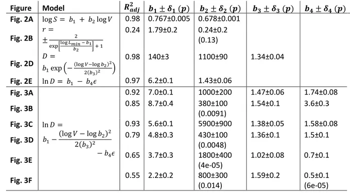
Figure Model 𝑹𝒂𝒅𝒋𝟐 𝒃𝟏± 𝜹𝟏 (𝒑) 𝒃𝟐± 𝜹𝟐 (𝒑) 𝒃𝟑± 𝜹𝟑 (𝒑) 𝒃𝟒± 𝜹𝟒 (𝒑) Fig. 2A log 𝑆 = 𝑏1 + 𝑏2log 𝑉 0.98 0.767±0.005 0.678±0.001
Fig. 2B 𝑟 =
± 2
exp[log 𝐿𝑚𝑖𝑛 − 𝑏1 𝑏2 ] + 1
0.24 1.79±0.2 0.24±0.2 (0.13) Fig. 2D 𝐷 =𝑏
1exp (−(log 𝑉−log 𝑏2)2 2(𝑏3)2 )
0.98 140±3 1100±90 1.34±0.04 Fig. 2E ln 𝐷 = 𝑏1 − 𝑏4𝜖 0.97 6.2±0.1 1.43±0.06
Fig. 3A
ln 𝐷 =
𝑏1−(log 𝑉 − log 𝑏2)2 2(𝑏3)2
− 𝑏4𝜖
0.92 7.0±0.1 1000±200 1.47±0.06 1.74±0.08
Fig. 3B 0.85 8.7±0.4 380±100
(0.0091)
1.54±0.1 3.6±0.3
Fig. 3C 0.93 5.6±0.1 5900±900 1.38±0.05 1.58±0.08
Fig. 3D 0.79 4.8±0.3 430±100
(0.0048)
1.36±0.1 1.5±0.1
Fig. 3E 0.65 3.7±0.3 1800±400
(4e-05)
1.02±0.08 0.7±0.1
Fig. 3F 0.55 2.2±0.2 800±300
(0.014)
1.59±0.2 0.5±0.1 (6e-05) 477
Table 1. Fitting parameters for figures in the main text. Parameter values 𝑏𝑖 are specified with 478
standard error 𝛿𝑖 and p-value in brackets (only when 𝑝 > 10−5). Fitting in Fig. 2B is done to the 479
outer hull of the data points.
480 481
15
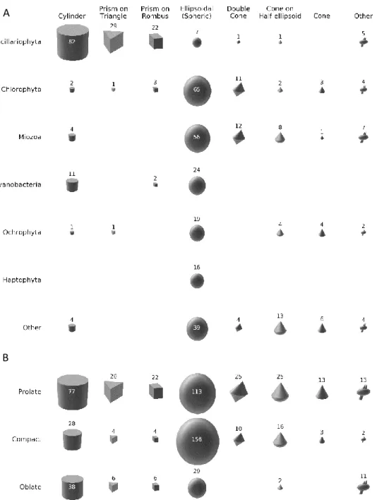
482
Fig. 1. Diversity distribution of various shape types (columns) across phyla (A, rows) and across cell 483
shape elongation (B, rows). The area of each figure is proportional to the number of genera (shown 484
next to or within it). See Extended Data Fig. 1 for detailed analysis.
485 486 487 488
A
B
16 489
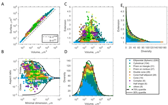
Fig. 2. Geometry of unicellular plankton for various cell shape types (A) Surface area as a function 490
of cell volume. The dashed, and dotted, lines show the slope of a power law fit, and a scaling with 491
the power of 2/3, respectively. (B) Aspect ratio, r, as a function of minimal cell dimension. The solid 492
line shows a fitted sigmoidal function to the upper boundary of | log 𝑟 | (black solid line). (C) Surface 493
relative extension as a function of cell volume. The dotted and dashed black lines show 75% and 90%
494
quantiles. (D) Distribution of taxonomic diversity as a function of cell volume. The black line shows a 495
fitted Gaussian function. (E) Distribution of taxonomic diversity over cell surface extension (note the 496
interchanged axes). The black line shows a fitted exponential function. The legend depicts the colour 497
coding for different shape types, with the number of genera for each shape type given in 498
parenthesis. See Table 1 for fitting parameters.
499 500
A
B
C E
D
17 501
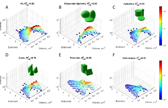
Fig. 3. Diversity distribution of unicellular phytoplankton. (A-F) Bivariate histograms of taxonomic 502
diversity, 𝐷, as a function of surface extension, 𝜖, and logarithm of cell volume, 𝑉, (dots), aggregated 503
over all shape types (A) and for different shape types (B-F). Note that due to intraspecific and 504
intragenus variability cells of the same genera can contribute to diversity in different bins. The mesh 505
(solid lines) shows a fit by the function ln 𝐷 = 𝑎 −(log 𝑉 − log 𝑉0)2/(2 𝜎2) − 𝛼𝜖, weighted with 506
diversity. The colours indicate taxonomic diversity from 𝐷 = 1 (blue) to 𝐷 = 200 (red) in A-C and to 507
𝐷 = 40 in D-F. See Table 1 for regression results, and Extended Data Fig. 7 for comparison between 508
predicted and observed diversity.
509
A B C
D E F
18
Extended Data
510
511
Extended Data Fig. 1. Diversity of phytoplankton across cell shapes (colour coded) and shape 512
elongation (top, middle and bottom panel) for different phyla (columns). See Methods for 513
classification of prolate, oblate and compact cells. Most of compact and prolate cells have cylindrical 514
or prismatic shape in Bacillariophyta, conic shapes in Cryptophyta and Charophyta, and ellipsoidal 515
shapes in the other phyla. Oblate cells are present in Bacillariophyta, Miozoa and Haptophyta, while 516
for the other phyla their frequency is less than 10%, in particular oblate cells absent in 517
cyanobacteria, Ochrophyta and Cryptophyta. Most of cylindrical and prismatic species belong to 518
Bacillariophyta. Bacillariophyta almost do not contain ellipsoids which have a large fraction in the 519
other phyla. Half-shapes (e.g. half-spheres or half-cones) are more dominated by oblate forms.
520
19 521
522
Extended Data Fig. 2. Bivariate effect of cell surface extension and aspect ratio on diversity. (A) 523
Distribution of taxonomic diversity (shown by colour) over aspect ratio (logarithmic binning) and 524
surface extension. The grey line shows a fitting parabola log 𝑟 = ±1.3√𝜖 − 1 to the upper boundary 525
of the aspect ratio for a given surface extension. Horizontal red lines at 𝑟 = 3/2 and 𝑟 = 2/3 show 526
the borders between compact, oblate and prolate cells, as defined in Methods. Diversity peaks for 527
compact cells with smallest sphericity (𝑟 = 1, 𝜖 = 1) and decreases both with increasing surface 528
extension and absolute value of logarithm of aspect ratio. (B) Distribution of taxonomic diversity 529
over aspect ratio. When projected on this axis the distribution of diversity shows peaks for cells with 530
𝑟 = 2 and 𝑟 = 1/2. We suppose that these peaks occur due to the specific shape of the distribution 531
in Fig. A, where aspect ratios of compact shapes can change very fast with a small increase in surface 532
extension, so the distribution is strongly stretched in the vertical direction resulting in a local minima 533
at 𝑟 = 1. (C) Distribution of taxonomic diversity over surface extension. In this projection the 534
diversity distribution decays exponentially.
535 536
A B
С
20 537
538
Extended Data Fig. 3. Prediction of surface extension and aspect ratio using various constraints on 539
linear cell sizes. To make a theoretical prediction of a potential variation in aspect ratio and surface 540
extension across cells we calculate the surface area and volume of ellipsoidal cells based on two 541
models: (i) assuming all three linear dimensions are log-uniformly distributed in the range from 1 to 542
1000 𝜇𝑚 and (ii) additionally assuming that the aspect ratio is constrained, 𝐿𝑚𝑎𝑥/𝐿𝑚𝑖𝑛< 100 for 543
prolate cells and 𝐿𝑚𝑎𝑥/𝐿𝑚𝑖𝑛< 40 for oblate cells. (A) Comparison of the aspect ratio of prolate (red 544
circulars) and oblate (blue circulars) cells with outer hulls for volume and aspect ratio in the first 545
model (black line) and in the additionally constrained model (black dashed line). (B, C) the same for 546
combinations of volume and surface extension for prolate (B) and oblate (C) cells. The first model, 547
assuming only that cell dimensions can vary from 1 to 1000 𝜇𝑚, reproduces the hump-shaped 548
dependence of maximal aspect ratio and elongation on volume (black solid lines show the outer 549
hulls across 50,000 ellipsoids with randomly chosen linear dimensions), but this model strongly 550
overestimates the maximal possible aspect ratio (ranges from 10-3 to 103) and surface extension 551
(achieves 20 for prolate ellipsoids and more than 30 for oblate ellipsoids). The second model, with 552
an additional constraint on cell aspect ratio, makes a relatively good prediction of the variation of 553
aspect ratio and surface extension as a function of volume for prolate cells, but it overestimates the 554
aspect ratio and surface extension for oblate cells. In particular, the model predicts that surface 555
extension for oblate species can reach 5, while the observed maximal surface extension for oblate 556
cells equals 2 for cells with intermediate.
557 558 559
A B C
Prolate Oblate
21 560
Extended Data Fig. 4. Dependence of the geometry of unicellular plankton on cell volume for 561
different nutritional modes. (A) Surface extension and (B) aspect ratio for different heterotrophic 562
groups of plankton cells (colour coded are autotrophs, mixotrophs and heterotrophs) in dependence 563
of cell volume. Based on data from Baltic sea, because only this data contained information on 564
trophic levels of organisms.
565 566
A
B
22 567
Extended Data Fig. 5. Distribution of taxonomic diversity as a function of volume for the most 568
common shapes partitioned by phyla groups. Black lines show a least square fit of a Gaussian 569
function 𝐷 = 𝑎 exp (−(log 𝑉−log 𝑉0)2
2𝜎2 ) to the histogram (see Extended Data Table 1 for fitting 570
parameters).
571 572
A B C
D E F
23 573
Extended Data Fig. 6. Distribution of taxonomic diversity as a function of surface extension for the 574
most common shapes types partitioned by phyla. Solid lines show a least square fit of a linear 575
function ln 𝐷 = 𝑎 − 𝑘𝜖 to the log-transformed histogram (see Extended Data Table 1 for fitting 576
parameters).
577
How correlations obtained across all shapes (𝑅2= 0.96) can be larger that those obtained for 578
specific shapes? The diversity distribution of elliptical genera (Fig. B) abruptly decreases with 𝜖 and 579
elliptical genera have a strong tendency to be compact (𝜖 ≈ 1). The maximum of diversity 580
distribution for cylindrical and conic genera occurs at 𝜖 ≈ 1.2 (Fig. C,D). Finally, the diversity 581
distributions of prismatic and other genera (Fig. E,F) decreases much slower with 𝜖 and exhibit some 582
secondary maxima. This can be interpreted as a kind of niche separation between shapes classes 583
along the gradient of surface extension. This niche separation diminish the quality of fit for each 584
specific shape class, but it is not visible any more when we consider the entire distribution (Fig. A).
585
The same explanation is applied for Fig. 3 (main text).
586 587 588
A B C
D E F
24 589
Extended Data Fig. 7. Comparison of observed diversity and diversity predicted based on nonlinear 590
regression models in Fig. 3 (blue dots). Black dashed lines shows 1:1 diagonals and solid lines are 591
linear regressions through the data points. The closer the solid line is to the dashed line, and the 592
smaller the variability of datapoints around this line, the better is the prediction of diversity by the 593
model function 𝐷 = 𝑎 exp(−(log 𝑉 − 𝑣0)2/(2 𝜎2) − 𝑘𝜖) in Fig. 3 (main text). An increase in the 594
variation of the predicted diversity in the range of small 𝐷 can partly be explained by the fact that 595
observed 𝐷 is constrained by 1, while predicted values can be less than 1. The regression analysis 596
shows that the predictions for ellipsoidal (B), cylindrical (C) and conic (D) shapes are unbiased, 597
because the solid and dashed lines are almost parallel. By contrast, for prismatic (E) and other 598
shapes (F) the regression lines deviate from the diagonals, and the model is biased as predictions of 599
diversity in the range of small observed 𝐷 are overestimated. However, as prismatic and other 600
shapes are relatively rare, the model provides also a good and unbiased prediction of diversity 601
across all shapes (A).
602 603
A B C
D E F
25 604
Extended Data Fig. 8. Diversity distribution of unicellular phytoplankton. Bivariate histogram of 605
taxonomic diversity as a function of aspect ratio and volume. To reduce the number of fitting 606
parameters the aspect ratio here is measured as 𝐿𝑚𝑎𝑥/𝐿𝑚𝑖𝑛, so that no distinction between prolate 607
and oblate cells has been made. Note that due to intraspecific and intragenus variability cells of the 608
same genera can contribute to diversity in different bins. To provide a better fit for prismatic and 609
other shapes (E, F), where diversity peaks at intermediate values of the aspect ratio, we also 610
assumed a Gaussian dependence on the aspect ratio. See Extended Data Table 1 for the results of 611
regression analysis.
612 613
A B C
D E F
26 614
615
Extended Data Fig. 9. The same as in Extended Data Fig. 6 but plotted as a function of the 616
logarithm of the cell aspect ratio.
617 618
A B
D E C
F
27
Figure Model 𝑹𝒂𝒅𝒋𝟐
𝒃𝟏± 𝜹𝟏 (𝒑) 𝒃𝟐± 𝜹𝟐 (𝒑) 𝒃𝟑± 𝜹𝟑 (𝒑) 𝒃𝟒± 𝜹𝟒 (𝒑) 𝒃𝟓± 𝜹𝟓 (𝒑) Ext. Fig. 5A
𝐷 = 𝑏1exp (−(log 𝑉 − log 𝑏2)2 2(𝑏3)2 )
0.98 155±4 1100±100 1.36±0.04
Ext. Fig. 5B 0.96 73±3 330±40 1.25±0.06
Ext. Fig. 5C 0.98 50±1 8700±800 1.17±0.04
Ext. Fig. 5D 0.85 24±2 400±10 (10−3) 1.19±0.1
Ext. Fig. 5E 0.72 22±2 (1.5e-05) 1200±40 (10−2) 1.07±0.2 (10−4)
Ext. Fig. 5F 0.76 6.9±0.5 900±30 (10−2) 1.36±0.2 (10−5)
Ext. Fig. 6A
ln 𝐷 = 𝑏1 − 𝑏4𝜖
0.96 6.6±0.2 1.50±0.06
Ext. Fig. 6B 0.8 6.3±0.6 2.4±0.3
Ext. Fig. 6C 0.92 5.2±0.2 1.36±0.08
Ext. Fig. 6D 0.77 4.3±0.3 1.2±0.1
Ext. Fig. 6E 0.71 4.0±0.3 0.95±0.1
Ext. Fig. 6F 0.62 2.6±0.3 0.75±0.1
Ext. Fig. 7A
ln 𝐷𝑝𝑟𝑒𝑑= 𝑏1+ 𝑏2ln 𝐷𝑜𝑏𝑠
0.85 0.1±0.1 (0.44) 0.99±0.05
Ext. Fig. 7B 0.66 -0.1±0.3 (0.74) 1.2±0.2
Ext. Fig. 7C 0.87 0.1±0.1 (0.41) 0.98±0.06
Ext. Fig. 7D 0.65 0.3±0.2 (0.11) 0.9±0.1
Ext. Fig. 7E 0.54 0.6±0.1 (1e-04) 0.6±0.1
Ext. Fig. 7F 0.54 0.4±0.08 (5e-05) 0.6±0.1
Ext. Fig. 8A
ln 𝐷 = −(log 𝑉 − 𝑏1)2
2 (𝑏2)2 + 𝑏3− 𝑏4𝑟
0.89 3.09±0.06 1.37±0.04 5.2±0.07 1.58±0.09
Ext. Fig. 8B 0.86 2.7±0.1 1.47±0.07 4.8±0.1 3.18±0.3
Ext. Fig. 8C 0.75 3.76±0.08 1.26±0.06 4.2±0.1 1.39±0.1
Ext. Fig. 8D 0.76 2.5±0.1 1.4±0.1 3.5±0.1 1.78±0.2
Ext. Fig. 8E
ln 𝐷 = −(log 𝑉 − 𝑏1)2
2 (𝑏2)2 −(log 𝑉 − 𝑏1)2 2 (𝑏2)2
0.66 3.18±0.09 1.03±0.08 2.7±0.1 0.91±0.05 0.56±0.05
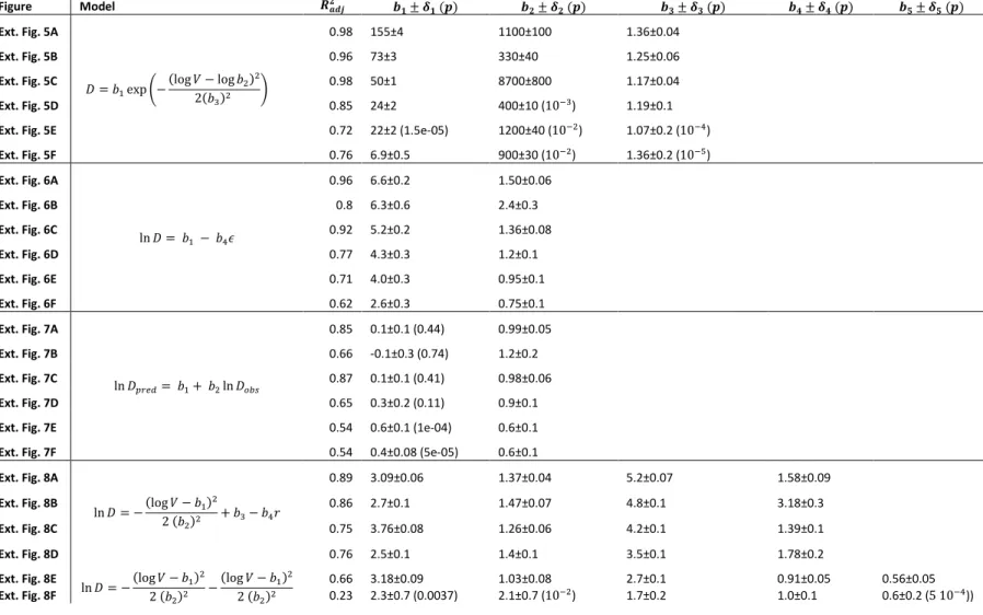
Ext. Fig. 8F 0.23 2.3±0.7 (0.0037) 2.1±0.7 (10−2) 1.7±0.2 1.0±0.1 0.6±0.2 (5 10−4))
Extended Data Table 1. Fitting parameters for figures in the Extended Data. Parameter values are specified with standard error, p-value in brackets is shown only when 𝑝 > 10−5.