article, distributed under the terms of the Creative Commons Attribution licence (http://creativecommons.
org/licenses/by/4.0/), which permits unrestricted re-use, distribution, and reproduction in any medium, provided the original work is properly cited.
THE INTCAL20 NORTHERN HEMISPHERE RADIOCARBON AGE CALIBRATION CURVE (0–55 CAL kBP)
Paula J Reimer1* •William E N Austin2,3•Edouard Bard4,†•Alex Bayliss5 •
Paul G Blackwell6•Christopher Bronk Ramsey7,† •Martin Butzin8,‡ •Hai Cheng9,10 • R Lawrence Edwards10,11•Michael Friedrich12•Pieter M Grootes13•
Thomas P Guilderson14,15•Irka Hajdas16,† •Timothy J Heaton6,† •
Alan G Hogg17,† •Konrad A Hughen18 •Bernd Kromer19•Sturt W Manning20 • Raimund Muscheler21,† •Jonathan G Palmer22 •Charlotte Pearson23 •
Johannes van der Plicht24•Ron W Reimer1•David A Richards25,†•E Marian Scott26 • John R Southon27•Christian S M Turney22 •Lukas Wacker16 •Florian Adolphi28,‡ • Ulf Büntgen29,30,31,32,‡•Manuela Capano4,‡ •Simon M Fahrni27,33,‡•
Alexandra Fogtmann-Schulz34,‡• Ronny Friedrich35,‡• Peter Köhler8,‡ • Sabrina Kudsk34,‡•Fusa Miyake36,‡•Jesper Olsen37,‡ •Frederick Reinig30,‡• Minoru Sakamoto38,‡• Adam Sookdeo16,22,‡ •Sahra Talamo39,‡
1The14CHRONO Centre for Climate, the Environment and Chronology, School of Natural and Built Environment, Queen’s University Belfast BT7 1NN, UK
2School of Geography & Sustainable Development, University of St Andrews, St Andrews, KY16 9AL, UK
3Scottish Association for Marine Science, Scottish Marine Institute, Oban, PA37 1QA, UK
4CEREGE, Aix-Marseille University, CNRS, IRD, INRA, Collège de France, Technopôle de l’Arbois, Aix-en-Provence, France
5Historic England, 25 Dowgate Hill, London, EC4R 2YA UK
6School of Mathematics and Statistics, University of Sheffield, Sheffield S3 7RH, UK
7School of Archaeology, University of Oxford, 1 South Parks Road, Oxford OX1 3TG, UK
8Alfred-Wegener-Institut Helmholtz-Zentrum für Polar-und Meeresforschung (AWI), 27515 Bremerhaven, Germany
9Institute of Global Environmental Change, Xi’an Jiaotong University China, Xi’an, 710049, China
10Department of Earth and Environmental Sciences, University of Minnesota, Minneapolis, MN 55455-0231, USA
11School of Geography, Nanjing Normal University, Nanjing, China
12University of Hohenheim, Hohenheim Gardens (772), 70599 Stuttgart, Germany
13Institute for Ecosystem Research, Kiel University, Kiel, Germany
14Center for Accelerator Mass Spectrometry L-397, Lawrence Livermore National Laboratory, Livermore, CA 94550, USA
15Ocean Sciences Department, University of California–Santa Cruz, Santa Cruz, CA 95064, USA
16Laboratory of Ion Beam Physics, ETH, Otto-Stern-Weg 5, CH-8093 Zurich, Switzerland
17Radiocarbon Dating Laboratory, University of Waikato, Private Bag 3105, Hamilton, New Zealand
18Department of Marine Chemistry & Geochemistry, Woods Hole Oceanographic Institution, Woods Hole, MA 02543, USA
19Institute of Environmental Physics, Heidelberg University, 69120 Heidelberg, Germany
20Cornell Tree Ring Laboratory, Cornell University, Ithaca, NY 14853, USA
21Quaternary Sciences, Department of Geology, Lund University, Sölvegatan 12, 223 62 Lund, Sweden
22Chronos 14Carbon-Cycle Facility, the Changing Earth Research Centre, and School of Biological, Earth and Environmental Sciences, University of New South Wales, Sydney, NSW 2052, Australia
23The Laboratory of Tree-Ring Research, University of Arizona, Tucson AZ 85721-0400, USA
24Centrum voor Isotopen Onderzoek, Rijksuniversiteit Groningen, Nijenborgh 6, 9747 AG Groningen, Netherlands
25School of Geographical Sciences, University of Bristol, Bristol BS8 1SS, UK
26School of Mathematics and Statistics, University of Glasgow, Glasgow G12 8QS, Scotland
27Department of Earth System Science, University of California–Irvine, Irvine, CA 92697, USA
†IntCal Focus group chair
‡Guest contributor
28Climate and Environmental Physics, Physics Institute & Oeschger Centre for Climate Change Research, University of Bern, Sidlerstrasse 5, 3012 Bern, Switzerland
29Department of Geography, University of Cambridge, Cambridge CB2 3EN, UK
30Swiss Federal Research Institute (WSL), 8903 Birmensdorf, Switzerland
31Global Change Research Centre (CzechGlobe), 603 00 Brno, Czech Republic
32Department of Geography, Faculty of Science, Masaryk University, 613 00 Brno, Czech Republic
33Ionplus AG, 8953 Dietikon, Switzerland
34Department of Geoscience, Aarhus University, Høegh-Guldbergs Gade 2, 8000 Aarhus C, Denmark
35Curt-Engelhorn-Centre Archaeometry, Mannheim, Germany
36Institute for Space-Earth Environmental Research, Nagoya University, Nagoya, Japan
37Aarhus AMS Centre (AARAMS), Department of Physics and Astronomy, Aarhus University, Ny Munkegade 120, 8000 Aarhus C, Denmark
38National Museum of Japanese History, Sakura, Japan
39Dept. of Chemistry G. Ciamician, Alma Mater Studiorum, University of Bologna, Via Selmi 2, 40126 Bologna, Italy
ABSTRACT. Radiocarbon (14C) ages cannot provide absolutely dated chronologies for archaeological or paleoenvironmental studies directly but must be converted to calendar age equivalents using a calibration curve compensating for fluctuations in atmospheric14C concentration. Although calibration curves are constructed from independently dated archives, they invariably require revision as new data become available and our understanding of the Earth system improves. In this volume the international14C calibration curves for both the Northern and Southern Hemispheres, as well as for the ocean surface layer, have been updated to include a wealth of new data and extended to 55,000 cal BP. Based on tree rings, IntCal20 now extends as a fully atmospheric record to ca.
13,900 cal BP. For the older part of the timescale, IntCal20 comprises statistically integrated evidence from floating tree-ring chronologies, lacustrine and marine sediments, speleothems, and corals. We utilized improved evaluation of the timescales and location variable 14C offsets from the atmosphere (reservoir age, dead carbon fraction) for each dataset. New statistical methods have refined the structure of the calibration curves while maintaining a robust treatment of uncertainties in the 14C ages, the calendar ages and other corrections. The inclusion of modeled marine reservoir ages derived from a three-dimensional ocean circulation model has allowed us to apply more appropriate reservoir corrections to the marine14C data rather than the previous use of constant regional offsets from the atmosphere. Here we provide an overview of the new and revised datasets and the associated methods used for the construction of the IntCal20 curve and explore potential regional offsets for tree- ring data. We discuss the main differences with respect to the previous calibration curve, IntCal13, and some of the implications for archaeology and geosciences ranging from the recent past to the time of the extinction of the Neanderthals.
KEYWORDS:calibration curve, radiocarbon, IntCal20.
INTRODUCTION
In most radioactive isotope systems used for dating, a daughter product is available for measurement so that an absolute age can be calculated. Unfortunately, for radiocarbon (14C) dating, this is not the case as the nitrogen produced by14C decay is not captured in most materials and, even if it were, this decay product would be swamped by the pervasive nature of nitrogen in the Earth system. Therefore, calibration against
14C measurements from known-age or independently dated material is critical for providing a correction for changes in 14C concentration within atmospheric and marine carbon reservoirs.
The IntCal Working Group (IWG) has endeavored to provide 14C calibration curves at semi-regular intervals since 2004, building on pioneering work by Stuiver et al. (1986, 1998a). Each new curve release incorporated all calibration data available at the time of construction that met the IntCal criteria (Reimer et al. 2013a) using robust curve construction methods. Inevitably, new datasets and improved understanding of the natural fluctuations in 14C in the atmosphere and oceans have resulted in an ongoing process of refinement, with curves (or particular datasets) becoming obsolete over time
*Corresponding author. Email:p.j.reimer@qub.ac.uk.
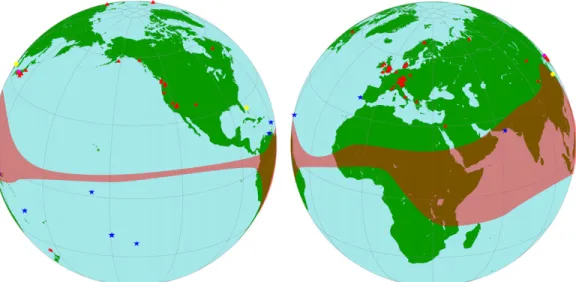
and replacement versions being released. In this latest iteration of the Northern Hemisphere IntCal curve, several new screening procedures were introduced to increase the transparency of data and metadata associated with a large influx of, mostly, annually resolved 14C measurements from tree rings. Including the large number of these data points that meet the published IntCal criteria (Reimer et al. 2013a) and the additional screening procedures described below, allows for wider geographic coverage in the tree-ring datasets than in previous versions (Figure 1) and improves the data density, and thus robustness, of the calibration curve. Equally importantly, the new approach makes subtle alterations to the shape of the curve for a more accurate representation of 14C concentrations across selected time periods not previously possible using multiyear tree-ring samples (blocks).
Beyond the last 12,310 years for which securely dated tree-ring data are available, annual and multiyear tree-ring data from floating sequences offer new ways to resolve and secure coarser-resolution paleoenvironmental sequences. Thus, back to ca. 13,910 cal BP, where sufficient, continuous 14C measurements of tree-ring chronologies exist, IntCal20 is fully atmospheric. For the older part of the timescale it was decided that the revised and extended atmospheric Lake Suigetsu varved sediment macrofossil record still lacked sufficient corroboration to be used as a stand-alone atmospheric record. Thus, this part of IntCal20 comprises statistically integrated evidence from floating tree-ring chronologies, terrestrial macrofossils from lake sediments, foraminifera from marine sediments, speleothems, and corals, using improved evaluation of the time and location variable 14C offsets from the atmosphere (reservoir ages, dead carbon fractions) for each dataset. All these data have been combined using a newly developed Bayesian spline approach which has been adapted to optimize the incorporation of a large number of annual tree rings.
IntCal20 is one of a collection of three calibration curves. IntCal20 is intended for the calibration of Northern Hemisphere atmospheric samples; SHCal20 the calibration of Southern Hemisphere atmospheric samples (Hogg et al. 2020 in this issue); and Marine20
Figure 1 Global representation of the datasets included in the Northern Hemisphere IntCal20 calibration curve: tree rings (red triangles), marine (blue stars), speleothem (yellow circles), Lake Suigetsu (magenta circle). The extent of the Inter-Tropical Convergence Zone (ITCZ) is shown as a shaded band after the reconstruction of the zonal boundaries based on wind data Hogg et al. (2020in this issue). (Please see electronic version for color figures.)
(with application of a local reservoir adjustment) the calibration of marine samples (Heaton et al.2020a in this issue).
THE DATASETS
The IWG has compiled an extensive database of published and previously unpublished data for the construction of the new curves which is available athttp://intcal.org. A list of the datasets included in the northern hemispheric curve and references for these datasets are given in Table S2. Some corrections to datasets included in previous IntCal curves have been made and are given here or in accompanying papers. The details of the datasets used for the Southern Hemisphere calibration curve SHCal20 and any special considerations are given in Hogg et al. (2020 in this issue). All ages in this paper and the database are reported relative to AD 1950 (= 0 BP, before present). Conventional 14C ages are given in units
“BP”and calendar or calibrated ages as“cal BP”or cal kBP (thousands of calibrated years before present). Historical AD/BC dates (without the year zero) are also used for known age events and dendrochronological dated wood in some cases. Further, all quoted uncertainties on values or offsets, e.g. 14±314C yr, refer to the 1σ level.
Terrestrial14C Archives and Considerations Tree Rings
Data criteria. A total of 220 tree-ring datasets from both published and previously unpublished sources were screened for possible inclusion in the IntCal20 curve for the Northern Hemisphere. Where possible, the research group that had produced each dataset was asked whether they considered their data suitable for inclusion in IntCal20. A number of datasets were either rejected at this stage (because of known problems with dendrochronology, the dissection of tree-ring series for 14C dating, the laboratory measurement, or the extant laboratory archive), or reserved for comparison purposes (e.g. where laboratories considered that higher quality data was available for a particular time period, or a laboratory problem was suspected but is still under investigation).
Datasets were then assessed against the relevant published IntCal criteria (Reimer et al.2013a):
1. Laboratory methodologies a. Pretreatment is specified,
b. Evidence of background or blank correction is provided, c. Details of uncertainty calculations are provided,
d. Data from relevant intercomparison exercises, known-age samples, or reproducibility with existing calibration datasets are provided.
In addition, all new data accepted into IntCal20 were required to include all quantifiable sources of uncertainty either through a laboratory error multiplier or additional variance.
All laboratories provided at least some information covering all these categories. Pretreatment was generally fully specified, but the level of detail of background or blank correction and uncertainty calculations varied greatly between laboratories. Approaches to replication also varied. Overall more than one measurement on the same cellulose preparation is available for ca. 10% of dated tree-ring samples, although more than 95% of these are
intra-laboratory replicates undertaken by QL- (set 1) and ETH- (set 69). Whole-process intra- laboratory replicates are available for only ca. 3% of dated tree-ring samples, almost 60% of which were undertaken by UCIAMS- (set 8), although inter-laboratory replicates are available for another ca. 3% (Usoskin et al.2013; Bayliss et al.2020in this issue; A. Sookdeo, personal communication; Pearson et al.2020in this issue; Friedrich et al.2020in this issue).
2. Dendrochronology
a. Sample derives from a single tree, b. Methodology used for dating is specified,
c. Details of ring(s) sampled in a particular tree are specified, d. Cross-matching of tree ring-width series is fully documented,
e. Cross-dating of tree ring-width series is fully documented (including version of reference chronologies used),
f. Raw ring-widths are published or deposited in a secure publicly accessible archive.
The criteria were expanded for this iteration of the curve to include dendrochronologies derived fromδ18O pattern matching. This can be used in the same way as ring-width dendrochronology to produce tree-ring sequences on a calendar timescale and tested using similar statistical criteria to those employed for traditional tree-ring dating (Nakai et al. 2018; Loader et al.2019).
A concerted effort was made to gather the required information for every new dataset under consideration for IntCal20 (and we thank the many dendrochronologists from all around the world who resolved our queries). At this stage, a number of datasets were rejected either because the dendrochronology was considered to be insecure or the dissection of the tree-ring series for14C dating was problematic. Other datasets have been reserved for comparison purposes (when insufficient information on the dendrochro- nology was available to us). Generally, considerable confusion was caused by the use of Historical BC (without a year zero) and Astronomical BC (with a year zero) in different laboratories and by different tree-ring software packages. It is essential that the calendar scale used is clear.
At this stage a small number of amendments/corrections were made to datasets that had been included in IntCal13:
1. Inconsistencies in block definition (e.g. which rings were sampled) were identified for the Amstel Castle data (van der Plicht et al. 1995; dataset 4/2), which could not be resolved and so this dataset has been removed from IntCal20.
2. A small number of data points in the Heidelberg datasets have been corrected (dataset 5/5, n=26) or withdrawn (dataset 5/3, n=5). Duplicate data in dataset 5/4 has been removed (see below).
3. In previous IntCal curves the Kodiak Island (KI) tree14C data were corrected for a 14±3
14C yr offset between a tree growing on Kodiak Island, Alaska (dataset 1/1) and Washington state (Stuiver and Braziunas1998). However, in IntCal20 the dataset’s scaled deviation and mean offset as estimated during screening (see below) did not flag this as being an outlier.
This correction was therefore not applied in IntCal20.
Because of the large amount of new data under consideration, particularly from 0 to 3000 cal BP, a minimum length for datasets was adopted to allow a realistic assessment of their reliability against existing datasets (10 measurements for decadal samples, 15 for 5-ring samples, 20 for 3-ring samples or 100 for single-year data, if not replicated by a second laboratory). An exception to the dataset length requirement was made for short series from laboratories also producing long datasets that passed the screening requirements. Another exception was data from the 14C spike events (Miyake et al. 2012, 2013) that had been replicated worldwide by numerous laboratories.
Twenty of the new datasets under consideration did not meet these length criteria and have been retained as comparison datasets. An unpublished dataset of three 10-ring samples of Irish oak from 3450–3470 cal BP (measured at the Center for Accelerator Mass Spectrometry, Lawrence Livermore National Laboratory) that was included in IntCal13, was also too short and redundant with all the new single-year measurements in the same time period (e.g. Pearson et al.2018,2020in this issue).
As a primary screening exercise, a preliminary curve was estimated using all the data under initial consideration. For each14C constituent dataset the scaled deviation (consisting of the sum of the scaled residuals) and the mean offset from this preliminary curve were calculated. This highlighted data which indicated potential inconsistencies relative to the other datasets and required further consideration. For those datasets with large scaled deviations (as assessed by a p-value) and high mean offsets, the authors were contacted and in most cases indicated there was a problem with the measurements that had not been resolved; hence these data are not included.
After this initial stage of screening, the process was repeated whereby another preliminary curve was created, but without those datasets excluded by the first screening. The p-values for the scaled deviations and mean residuals were re-calculated flagging up datasets that needed further individual consideration by the group. This was performed by visual inspection of plots and discussion within the group ending with a vote on inclusion. Data which were judged to be too scattered were excluded from the curve including Irish oak data published by McCormac et al. (2008; dataset 2/6), which had been included in IntCal09 and IntCal13.
Two further categories of data were excluded from IntCal20: (1) a small number of recent datasets which appeared to be depleted in 14C resulting from the use of fossil fuels during the industrial revolution (Tans et al. 1979), and (2) datasets within or at the present day limit of the Inter-tropical Convergence Zone (ITCZ, see below). An inter-laboratory tree- ring dating comparison led by L. Wacker was organized by the IntCal Dendrochronology focus group. The anonymized results of this comparison are presented in Wacker et al.
(2020 in this issue) and provide insights into the accuracy and quality of high-precision measurements on single tree rings performed by the participating AMS laboratories. The Holocene measurements obtained by AMS are comparable in quality to the ones previously performed by decay counting (Stuiver et al. 1998a), though requiring several orders of magnitude less material, whereas during the late glacial (ca. 15–11.7 cal kBP), AMS measurements in IntCal20 are superior to previous decay counting results (Sookdeo et al. 2019in this issue). As with previous calibration curves, some of the tree-ring datasets included in the curve are more variable than the quoted uncertainties would indicate i.e. 14C determinations arising from tree rings with identical calendar years appear more
widely spread than would be supported by their reported uncertainties. We call this additional variability over-dispersion. Rather than include a laboratory error multiplier as was done in the past, an additive error to correct for potential over-dispersion in the IntCal20 measurements was built into the Bayesian statistical method (Heaton et al.2020b in this issue). By specifically including such an additive term to model over-dispersion we aimed to correct not only for any potential under-reporting of laboratory measurement error within the IntCal20 datasets but also potential dispersion caused by intra-hemispheric locational offsets and other inter-tree variation. A prior probability distribution (hereafter prior) for the level of over-dispersion was formed based upon inter-lab variability of the same tree-ring samples produced for the Sixth International Radiocarbon Intercomparison (SIRI, Scott et al.2017b). This prior was expected to be somewhat conservative for the IntCal20 data (i.e. indicate a greater level of over-dispersion) due to the much wider set of AMS laboratories participating in SIRI than used for IntCal20. However, due to the large volume of IntCal20 data, our posterior estimate for the over-dispersion is dominated by the high quality IntCal20 data themselves.
The posterior estimate for the over-dispersion within the Northern Hemisphere IntCal20 datasets can be seen in Heaton et al. (2020b in this issue, Figure 5). Anticipating similar levels of over-dispersion amongst the14C determinations users wish to calibrate, to improve calibration accuracy, this posterior is incorporated into our published curve through the creation of predictive intervals.
Consideration of regional and seasonal growth offsets in tree-ring 14C. While 14C offsets between the Southern and Northern Hemispheres are well documented (McCormac et al.
1998; Stuiver and Braziunas1998; Hogg et al.2009; Turney et al. 2016a), offsets within the Northern Hemisphere are less well understood. Intrahemispheric offsets were predicted by a global tracer transport model using ocean boundary conditions (Braziunas et al. 1995) to be on the order of 8 14C yr or less in the Northern Hemisphere except at very high latitudes (>70°N). However, offsets could also result, in theory, from the location of the tree relative to the ITCZ and monsoons, growing season differences, polar latitudes, proximity to upwelling of 14C-depleted ocean water, proximity to industrial centers, and high altitude. Regional offsets within a hemisphere can be difficult to corroborate, as they are of a scale similar to observed inter-laboratory variation (Wacker et al. 2020 in this issue; Friedrich et al. 2020 in this issue; Pearson et al. 2020 in this issue) but have been observed convincingly in a few cases (Turney et al. 2016a; Büntgen et al. 2018; Pearson et al.2020in this issue).
The ITCZ is an asymmetric area of low pressure around the thermal equator where the northeast and southeast trade winds converge. The ITCZ migrates on seasonal and longer timescales (Haug et al. 2001; Schneider et al. 2014). In extreme situations, the ITCZ appears to have experienced a major southward migration across Amazonia during Heinrich stadials (Cheng et al. 2013). Trees growing within the ITCZ are potentially subjected to air masses from different hemispheres at certain times of the year (Marsh et al.
2018; Hogg et al. 2020 in this issue). For example, Southern Hemisphere air masses in tropical and subtropical Brazil have been detected in 14C measurements from trees growing in the 1960s (Lisi et al.2001). Hua et al. (2004) similarly concluded that tropical trees from Thailand had lowered 14C levels because of the influence of Southern Hemisphere air masses. The authors reported an offset of 32 ± 8 14C yr for pine from north-central Thailand compared to trees from the northwest United States (Stuiver et al. 1998b) between AD 1690 and 1780. However, this appears to be primarily an inter-laboratory
effect, since the Thai data are younger than Tasmanian trees measured concurrently at the same laboratory (Hua et al. 2004) by 30 ± 8 14C yr for AD 1620–1780 (data presented in Table 1 in Hogg et al.2013a), which is identical to the interhemispheric offset for the same interval based on New Zealand cedar and British oak of 28–32±714C yr (Hogg et al.2002).
Tree-ring data from between or near the boundaries of the present day ITCZ (Figure1) were therefore not included in IntCal20 but retained in the database for comparison. These include measurements from pine trees from Thailand obtained inside the ITCZ (Hua et al. 2004;
Q. Hua, personal communication). In addition, a Tibetan juniper growing at 31ºN 91ºE (Büntgen et al. 2018), approximately at the northern boundary of the present day ITCZ, was not included because this dataset had a mean difference of 18.5 14C yr older compared to other IntCal datasets, which suggested a moderate influence of Southern Hemisphere air.
While altitude has been postulated as mechanism for increased14C in tree rings (Cain and Suess 1976), there is no evidence for this in more recent higher precision measurement of high elevation trees compared to low- and mid-elevation trees growing during 14C spike events (Büntgen et al. 2018). However, altitude is a factor in growing season differences. Northern Hemisphere seasonal differences in14C between plants growing in the early spring and later in the summer can come about because stratospheric 14C is injected into the troposphere during the boreal spring (Appenzeller et al. 1996; Stohl et al. 2003). For example, Dee et al. (2010) reported an offset of 19 ± 5 14C yr between short-lived herbaria specimens collected in Egypt between AD 1700 and 1900 and IntCal09. Other studies using blocked (multiyear) tree-ring data have indicated that differences may be enhanced during periods of low solar activity when 14C production is higher (Kromer et al. 2001). For example, Kromer et al. (2001) found only a minimal expected latitudinal offset between the14C ages of Turkish pines and German oak on average from AD 1420 and 1640 but the Turkish pines were older than the German oak by 17 years during the Spörer solar activity minimum. Dellinger et al. (2004) found deviations of up to 17 ± 5 14C yr for stone pine growing in the Alps between 3500 BC and 3000 BC compared to the low altitude tree-ring measurements that were included in IntCal98. Manning et al. (2018) also reported fluctuating regional offsets from AD 1610 to 1940 from trees growing in Jordan compared with IntCal13 averaging 19 ±314C yr, associated with periods of reversals and plateaus in the 14C calibration record. However, this average offset is reduced to less than 10 14C yr when compared to new datasets included in IntCal20 (L. Wacker, personal communication). Comparison of data from Germany and Turkey measured at the same laboratory—removing the issue of inter-laboratory variation as a cause—indicates similar fluctuating offsets in the period from the 17th to the 8th centuries BC that are again associated with reversals and plateaus in the14C calibration record (Manning et al.2020).
While the mentioned examples may overestimate regional offsets, the large influx of annual tree-ring data submitted to IntCal20 offers a range of new approaches to study this issue.
The results of a study of the global extent of cosmic events showed only slight differences between trees growing through a range of growth seasons across a range of environments during the years 774 and 993 AD and suggests only a slight latitudinal offset at these times (Büntgen et al. 2018: Fig.3). Pearson et al. (2018) reported Irish oak latewood representing mid-May through early autumn growth (Baillie1982) and North American bristlecone pine whole tree rings (representing June, July, August growth) which were within stated errors of one another in the period 1700–1500 BC. Pearson et al. (2020in this issue) refine this to
an average weighted mean difference of–8.1±1.914C yr between Irish and North American
14C data for this period. This is still within stated errors but may also reflect a slight latitudinal effect.
Future work on growing season differences and latitudinal dependences is therefore recommended along with exploration of other factors such as latitude or altitude.
Seasonality will be particularly important for tracking and defining any new discoveries of rapid excursions in atmospheric 14C concentration. For example, in the Southern Hemisphere, growth is split across two calendar years and for European oak, the earlywood is formed using photosynthates from the previous calendar year (Pilcher 1995).
Either of these could potentially aid in refining the timing of rapid (intra- and inter-annual) events. In regions north of the polar front, atmospheric14C may be elevated in late spring/
early summer due to stratospheric injection of 14C and therefore could, in theory, enrich the14C of trees growing north of the polar front. Stuiver and Braziunas (1998) found only a minimal Δ14C offset (–0.3 ± 0.7 ‰) for AD 1615–1715 but an offset of 26 ± 6 14C yr younger for AD 1545–1615 for a Siberian larch tree (67°N, 123°E) compared to a tree from Washington state (48°N, 124°W) which is in good agreement with Büntgen et al.
(2018). Data from northern Norway from trees growing during the peak of nuclear weapons testing also had higher 14C (Hua and Barbetti 2007; Svarva et al.2019) but may not be representative of natural offsets due to the high latitude of many of the atmospheric bomb tests. Büntgen et al. (2018) reported elevated 14C values for some trees growing above 60ºN at the peak of the AD 774/5 Miyake event (Miyake et al. 2012). The position of the present-day polar jet stream, which delineates the polar front, is presented as a latitudinal probability distribution by Molnos et al. (2017), but a simple boundary is not easily established. We therefore used 60ºN for comparison of northerly trees with the other data. We found only small offsets for most tree ring 14C data in the compilation above 60ºN so retained the following datasets for use in the curve: SWE02 (68.3°N, 19.6°E;
dataset 69/34), Kom1213175a/b (68.5°N, 20.0°E; dataset 60/4), RUS04 (67.5°N, 70.7°E;
dataset 69/42), and Yamal (67.5°N, 70.7°E; dataset 68/8). Büntgen et al. (2018) reported offsets between 12 ± 6 and 27 ± 5 14C yr younger for samples above 65°N measured at ETH. The potential for a latitudinal offset needs to be considered more carefully in the future.
Proximity to coasts with upwelling of older oceanic carbon has been proposed to cause14C offsets. As mentioned earlier, Stuiver and Braziunas (1998) found a 14 ± 3 14C yr offset between a tree growing on Kodiak Island, Alaska (KI tree; dataset 1/1), and those trees growing in Washington State, USA. 14C offsets between trees from Japan and the IntCal curves for several time periods have also been postulated to be due to ocean upwelling (e.g. Nakamura et al.2007). It is not clear if these latter observations are real or a product of inter-laboratory variation.
To summarize, regional 14C offsets can be difficult to determine due to measurement uncertainties and inter-laboratory offsets. Such analyses, however, are critical for future calibration curves, particularly to define the boundaries and changes through time of the ITCZ as well as growing season effects. 14C measurements of tropical trees would provide much needed information on the ITCZ, however, it can be difficult to obtain reliable dendrochronological dates due to the limited seasonality in the tropics and subsequent indistinct tree rings. Through the application of X-ray densitometry and confirmation
through14C measurements of trees growing during the nuclear weapons testing in the 1960s, chronology establishment was successful for some tropical species (Lisi et al.2001; Santos et al.
2015). This may provide an improved understanding of the offsets because of the higher14C levels (Hua and Barbetti2007).
Dataset updates. Irish oak data from the Waikato laboratory (Hogg et al. 2009) for the intervals AD 245−335, 745−785, and 895–935 had accidentally been left out of IntCal13 and are now included. Decadal German oak data from the Heidelberg laboratory for the period 1600–1700 BC were inadvertently entered twice with different laboratory ID’s in IntCal09 and IntCal13. This problem was corrected for IntCal20.
From IntCal04 through IntCal13 (Reimer et al. 2004, 2009, 2013b), laboratory error multipliers for the tree-ring data were calculated from the offset with Seattle (QL) measurements with an estimated 1.3 error multiplier applied. Although no correction was made to the data for the calculated offset as had been done in IntCal98 (Stuiver et al.
1998a) the error multipliers increased the uncertainty in the data.
The Seattle error multiplier was re-calculated from replicates using equation 2 from Scott et al.
(2017a). Of the replicates, 459 were duplicates, 35 were triplicates and there was 1 set each of quadruplets and quintuplets. The lab error multiplier (k) was calculated to be 1.07. Since the replicates were almost all aliquots of the same wood processed to alpha cellulose it was decided to leave the error multiplier at 1.3 which should encompass any additional variability such as a cellulose processing error. The laboratory error multipliers for the other legacy datasets were also left at the 2004 values with the exception of the more recent data from Belfast and Waikato where intra-laboratory multipliers had already been included in the reported uncertainties (McCormac et al. 2004; Hogg et al. 2009; datasets 2/1, 2/2, 3/1 and 3/2). The laboratory error multipliers for these datasets were therefore set to 1 in order not to apply the error multipliers twice.
A revised radon correction was applied to the Seattle data measured from 1977 to 1987 (Stuiver et al. 1998b). As an additional check on the revised radon correction, 10 decadal wood samples from a Douglas fir (S tree; dataset 1/10) from the Seattle laboratory were processed to cellulose by Fusa Miyake and measured by AMS in Belfast. Replicate AMS measurements on the cellulose were made on three samples to check potential outliers.
The results of the new S tree cellulose extractions are within one standard deviation from the Seattle radon corrected measurements of the S tree and a sequoia (RC tree) except for one sample at 995 cal BP (Figure S1; TableS1). These new replicate data have not been included in IntCal20.
Same cellulose replicates and processing error estimation. In order to avoid over-precise error estimates from averaging of replicates made on the same cellulose, a correction was made for cellulose processing differences. The cellulose processing error, in terms ofΔ14C, was estimated at 1‰(1σ; equivalently 814C yr) (L. Wacker, personal communication) and may be even less for the large carbon mass samples used for radiometric dates. For replicates, identified by the same laboratory identification number, the cellulose processing uncertainty was removed from the total uncertainty by subtracting 814C yr in quadrature. A weighted mean of the14C ages
was calculated with the uncertainty in the mean given by
1
1 σ12 σ1
22
s
whereσ1andσ2are the measurement uncertainties in the14C ages of the replicates. Finally, the cellulose processing error was added in quadrature to the uncertainty in the mean.
New measurements of single dendrochronologically dated tree rings. Publication of the rapid increase in atmospheric 14C in AD 774–775 (also known as the “Miyake event”) and the subsequently discovered AD 993 event (Miyake et al. 2013) has prompted 14C measurements on additional single tree rings from these time periods (e.g. Jull et al. 2014;
Büntgen et al. 2018; Kudsk et al. 2019 in this issue) and led to the search for additional unusual events that can be detected in annual or biannual measurements (e.g. Miyake et al.
2017a,2017b; Jull et al.2018). To incorporate the large amount of annual data that have been produced for several of these short time periods and to represent the rapid increases, additional knots in the spline were included at these points for calibration curve construction (Heaton et al.2020b in this issue).
Dating of the second millennium BC eruption of Thera (Santorini) has long been a contentious issue for Mediterranean archaeology. Bayesian models using the more recent iterations of IntCal have pointed to a late 17th century BC eruption, contrary to some interpretations of the archaeological and historical evidence which indicate a more recent eruption date (Kutschera et al. 2012; Manning et al. 2014; and references therein). A recent publication of single-year bristlecone pine and Irish oak samples (Pearson et al.2018) indicated that an annual calibration dataset might offer a new approach to this issue by refining the curve shape. IntCal13 was based on 20-, 10- and 5-ring samples of wood for this period and included a flat region or plateau. The annual calibration dataset has refined the definition of the plateau which is very important for establishing the true possible calendar age ranges for the key Theran datasets. Calibration models using a curve constructed in the same way as IntCal13 from the new bristlecone and oak data increased the probability of a more recent eruption (Pearson et al.2018). To test these multispecies tree-ring data, a number of laboratories have now analyzed contemporary tree rings at annual resolution (Friedrich et al.2020 in this issue; Kuitems et al.2020in this issue; Pearson et al. 2020 in this issue).
All the new data for this time period that were available at the time of the curve construction have been included in IntCal20. Implications for the dating of the Thera eruption are discussed in light of the IntCal20 curve in Friedrich et al. (2020in this issue), Pearson et al. (2020 in this issue), Kuitems et al. (2020 in this issue), and van der Plicht et al. (2020in this issue).
The Hallstatt plateau (ca. 800–400 BC), one of the largest flatter regions in the calibration curve, has been problematic for resolving 14C dating chronologies during a critical period in prehistorical technological developments in Europe and elsewhere without adequate stratigraphic control (Hamilton et al. 2015). Single-ring data from German oak and sequoia now provide detail for the first half of the Hallstatt plateau (2805–2575 cal BP) and increased the dating resolution across this key period (Park et al. 2017; Fahrni et al.
2020in this issue).
Annual data for the period 290–486 AD (1660–1464 cal BP) (Friedrich et al.2019) have also provided improved resolution of the IntCal raw data. These annual datasets demonstrate periodic changes in the annual records which may be attributed to the “11-year” Schwabe cycle (with a length from 9 to 11 years). They also show a ca. 20 14C yr offset from
IntCal13 for a part of the time period covered, which is not explained by regional/latitudinal differences but more likely indicates that the curve could be slightly improved by more highly resolved data for a part of this period.
Floating tree-ring sequences: changes and additions.A major inter-comparison exercise using late glacial floating kauri tree-ring sequences (Hogg et al.2016) resulted in a14C wiggle-match, with correction for the interhemispheric offset, to the European Preboreal Pine (PPC) chronology (Friedrich et al. 2004). This in turn indicated that the Swiss ZHYD-1 (formerly YD-B) record (Schaub et al. 2008; Hua et al. 2009; Kaiser et al. 2012) was incorrectly linked to the PPC. Tree-ring width reanalysis and annual resolution 14C measurements between 13,150 and 11,800 cal BP of previously collected Swiss trees (Kromer et al. 2004;
Schaub et al. 2008; Hua et al. 2009; Kaiser et al. 2012), as well as the recently discovered additional Swiss subfossil samples (Reinig et al. 2018), enabled the dendrochronological extension of the PPC (Reinig et al. 2020 in this issue), which is supported by 14C wiggle- matching (Sookdeo et al. 2019 in this issue). The new PPC extension was then used to more securely wiggle-match the floating kauri chronology (Hogg et al. 2016) which in turn was used to reposition ZHYD-1 and the German/Swiss Central European Lateglacial Master Chronology (CELM) record (A. Sookdeo, personal communication) thus extending it to 14,226 ± 4 cal BP. However, the last few decades of this chronology could not be sampled for 14C measurements. This new positioning was reinforced by the inclusion of single-year measurements of subfossil pine trees from the French Alps (Capano et al.2018, 2019in this issue) which strengthen the curve for this period.
Complementing the above, Adolphi et al. (2017) correlated three floating tree-ring chronologies from Northern Italy to ice core 10Be datasets for the Bølling chronozone (ca. 14,700–14,000 cal BP, equivalent to GI-1e1) which indicated that the IntCal13 curve was too smooth in this period. We have incorporated these datasets but matched to the14C of the rest of the calibration data rather than using the ice core ages to keep the timescales independent (Muscheler et al.2020in this issue).
Further back in time, a 2000-yr-long series of bidecadal measurements of a floating kauri tree- ring chronology spanning Heinrich Stadial 3 (ca. 30.6–28.9 cal kBP, equivalent to GS-5) from Finlayson Farm, New Zealand (Turney et al.2016b) were14C matched to the other calibration datasets by including an interhemispheric offset 43± 23 14C yr (Hogg et al. 2013b). These measurements provide added detail to the curve for HS-3/GS-5. A 1300-yr-long series on consecutive 100-ring samples from trees from Mangawhai Heads, New Zealand (Turney et al.2010) was also included and is discussed in Muscheler et al. (2020in this issue).
Plant Macrofossils
Plant macrofossils provide another possible sample type for calibration. The four characteristics to be considered in their application are (1) the reservoir from which their carbon originates, (2) the time period covered by their growth, (3) their preservation, and (4) the ability to provide an independent timescale. For atmospheric calibration this implies that the plant macrofossils should be from terrestrial rather than lacustrine or marine plant species and that they should either be from short-lived species or from annual growth of longer-lived species (leaves, needles and small twigs).
1Greenland interstadials (GI) and stadials (GS) equivalents are based on Rasmussen et al. (2014).
The preservation of such material is poor in many contexts but the anoxic conditions in some lake sediments allows for their preservation in a sufficiently good state for identification, and in sufficient density to provide a quasi-continuous record. Fortunately, such anoxic conditions, with minimal bioturbation can also result in annual layers or varves, which may additionally provide a (normally relative) independent timescale.
However, even in ideal circumstances, plant macrofossils do not allow the density of measurements, or the ability to undertake duplicate or high precision analyses that are afforded by tree rings. For this reason, although they do, like wood, provide a very direct measure of carbon in the atmosphere, they are only really useful for calibration in periods where wood is not available, or to provide a long-term record which spans a much longer timescale than any individual tree-ring series can. These considerations, along with the combination of criteria needed to make plant macrofossils a suitable material for 14C calibration, make suitable records very rare and only the Lake Suigetsu varved sediment macrofossil data (Bronk Ramsey et al. 2012) is included in the IntCal20 curve. It is useful because it provides the only quasi-continuous, truly atmospheric record older than ca.
14,190 cal BP, extending to the limit of the technique. This record has been reanalyzed with an extension and revision of the varve counting through to 50 cal kBP (Schlolaut et al. 2018). An updated timescale was modeled (Bronk Ramsey et al. 2020 in this issue) using both the new varve chronology and a 14C wiggle-match to the extended Hulu Cave record (Cheng et al.2018).
Speleothems
Speleothems are secondary carbonate mineral deposits formed in caves. Carbon, and hence
14C, in pristine calcite speleothems is derived from a variety of sources with a spectrum of
14C ages. In simplest terms, these are atmosphere, soil gas, soil organic matter and ancient limestone, the last of which is essentially devoid of14C and contributes to the dead carbon fraction (DCF; for a recent review see Markowska et al. 2019). The relative contributions of different carbon pools to speleothem calcite (or aragonite) is site-specific and depends on many factors in the karst geochemical setting that respond to changing local climate and vegetation. Controlling factors of DCF include the extent of open or closed system dissolution of the host rock (Hendy 1971), the spectrum of ages of soil organic matter (Fohlmeister et al.2011; Noronha et al. 2015), and influence of non-carbonic acids such as sulfuric acid (Bajo et al. 2017). Secular DCF variation is expected and numerous studies have indicated abrupt short-term variations related to climate change (e.g. Oster et al.
2010; Rudzka et al. 2011; Lechleitner et al. 2016), but the relative shifts are difficult to predict. To accommodate this, speleothem DCFs were modeled here as independent fluctuations around a constant mean. We placed a prior on the mean DCF for each speleothem based upon the period of speleothem growth that overlaps with tree ring records included in IntCal20 (Heaton et al. 2020b in this issue). This overlap additionally provided an estimate of the size of the independent fluctuations around this mean over time.
During curve construction we further updated these prior mean DCF values to resolve potential offsets between datasets and obtain posterior DCF estimates for each speleothem.
The Hulu Cave H82 speleothem14C record was utilized in IntCal13 from the end of the tree ring record at 14,153 cal BP to 26,850 cal BP (Southon et al. 2012). Recent14C and U-Th measurements on the Hulu Cave MSD and MSL speleothems overlap with the earlier measurements and provide new data to 53.9 cal kBP (Cheng et al. 2018). These speleothems were formed in a region of the cave underlying a portion of host rock for
which the original limestone has been largely replaced with iron oxides (not sandstone as originally reported by Cheng et al. 2018). Speleothem DCF is predicted to be low and, most critically, show only minor variation (Cheng et al. 2018) because the waters derive most of their dissolved inorganic carbon from soil CO2 and the lower sections of the vadose pathway, dominated by Fe-oxides, and see minimal contribution from deep-seated soil-organic matter derived CO2. δ13C values of these Hulu Cave stalagmites vary by several per mil (Kong et al. 2005). Notably, however, significant shifts inδ13C do not result in resolvable shifts in DCF (Southon et al. 2012). This decoupling can be explained by the fact that of the many well-known processes that control δ13C (Hendy 1971), a significant subset would not be expected to directly affect DCF. The latter includes shifts in overlying vegetation between C3 and C4 biomes, which is indeed invoked by Kong et al. (2005) to explain the δ13C variations observed at Hulu. In addition, the lack of nuclear weapons testing 14C in the cave dripwaters, as well as observed seasonal δ18O values, support a relatively short residence time of the soil carbon and infiltration into the cave (Cheng et al.2018).
Each Hulu Cave speleothem was permitted to have a potentially different DCF for the purposes of curve construction. A mean DCF value of 480 ±814C yr was used as a prior for each, with a further independent variation around this mean value in any particular calendar year of ±50 14C yr, based upon calculations from the overlap of H82 with the updated tree ring section of the IntCal20 curves. The slight difference from the DCF value, in any calendar year, of 450 ± 70 14C yr used by Cheng et al. (2018) is due to improvements in the tree-ring chronologies and additional measurements discussed above.
During curve construction, these DCF priors were updated and we obtained posterior DCF estimates of 472 ± 50 14C yr for H82, 470 ± 5014C yr for MSD, and 481 ± 50 14C yr for MSL respectively2. This demonstrates the DCF consistency across the three Hulu speleothems.
In addition, we utilize Bahamas speleothems which are represented in IntCal20 by two stalagmites collected in an underwater cave on Grand Bahama; GB89-24-1 (Beck et al.
2001) and GB89-25-3 (Hoffmann et al. 2010). The data from these speleothems were incorporated into IntCal13. GB89-25-3 was found broken with 4 basal pieces and 2 top pieces with an intermediate section being lost. Both samples exhibit growth that overlaps with tree ring sections to determine offset and uncertainty. Variation in DCF is greater than that observed in the Hulu speleothem H82. For GB89-24-1, the prior on the mean DCF value was 1515 ± 3214C yr, with an assumption of additional independent variation around this mean in any calendar year of ±207 14C yr. This prior was updated during curve construction to provide a posterior DCF estimate for GB89-24-1 of 1523±20814C yr. GB89-25-3 was treated as two separate sections. The prior for the mean DCF of the top sections was set at 2156± 3314C yr, with additional independent variation in any year of ±319 14C yr, based on overlap with tree ring sections. After curve construction, the posterior DCF for these top sections was estimated to be 2173 ±32014C yr. For the basal sections an uninformative prior on the mean DCF value was used allowing us to retain internal structure seen within this lower section but allow for a potential step change in DCF from the top sections. After curve construction, we obtained a posterior DCF for these basal section of 2891 ± 32314C yr (Heaton et al. 2020b in this issue). The large DCF uncertainties downweight the contribution of the Bahama speleothem records to the calibration curve. However, their inclusion is justified because
2In reporting the±1σuncertainty for all DCF posteriors, we have subsumed the uncertainty in the posterior mean DCF level into the uncertainty due to additional independent variation.
the agreement between two speleothem records (e.g. Hulu Cave and Bahamas) with very different locations and depositional contexts builds increased confidence in both records as discussed in Southon et al. (2012).
Marine14C Archives and Considerations
There are no new U-Th dated coral14C measurements available prior to the Holocene since the publication of the IntCal13 and Marine13 curves (Reimer et al. 2013b). However, despite adhering to the IntCal criteria (Reimer et al. 2013a), some of the coral data used in IntCal13 exhibit wide scatter in Δ14C (~500 ‰), especially around 37 kyr BP (Figure2). It is likely that diagenesis due to exposure to freshwater occurred when these corals were above sea level during the lowstand of the Last Glacial Maximum (LGM; 21±2 cal kBP).
This effect appears to have been particularly prevalent in corals from areas with rapid uplift such as Vanuatu for which coralΔ14C appears very elevated (>1100‰around 27–29 cal kBP; Cutler et al. 2004). In addition, a coral data point from Tahiti at 31 cal kBP is obviously an outlier as presented and discussed in Durand et al. (2013). It was therefore decided to remove all coral data older than 25 cal kBP for construction of the IntCal20 curves to avoid the potential inclusion of erroneous data. Further work is needed to develop a way of identifying which corals are affected by diagenesis.
As in IntCal13, the timescales for the marine foraminifera records from the Iberian margin, Pakistan margin and the Cariaco Basin were based on tie-pointing the rapid transitions
0 100 200 300 400 500 600 700 800 900
25000 30000
35000 40000
45000 50000
D14C (‰)
cal BP
Tahiti Papua NG Barbados Vanuatu IntCal20
Figure 2 Age-corrected coralΔ14C older than 25 cal kBP from Bard et al. (1990,1998,2004a) and Durand et al.
(2013) (Tahiti, Barbados, New Guinea), Cutler et al. (2004) (Vanuatu, Papua New Guinea) and Fairbanks et al.
(2005) (Vanuatu, Barbados) compared to IntCal20 (shown with 1-σuncertainty envelope). The coral data is not reservoir corrected but this is not relevant for illustrating the large variation in the coral data.
between stadial and interstadial events in the proxy climate records, assumed to be synchronous within an uncertainty of ±100 yr, to those in the Hulu Cave δ18O values (Wang et al.2001; Cheng et al.2016) using a Gaussian process model (Heaton et al.2013).
The assumption of synchronicity builds on our previous work focused on a few selected marine sites (see Hughen et al. 1996,2004a,2004b, 2006for the Cariaco Basin; Bard et al.
2004a, 2004b for the Iberian Margin; and Bard et al.2013 for the Pakistan Margin) and is supported by modeling results (e.g. Rind et al. 1986; Manabe and Stouffer 1995) showing tropical Atlantic and Asian responses to North Atlantic cooling, which suggests temporally rapid and spatially coherent changes across the area including the various climate archives.
For the sediment cores from the Pakistan and Iberian margins, the climate proxy records are the same as those described for IntCal13 (Bard et al.2013). The only significant difference is that the Iberian alkenone-SST record has been remeasured to increase its time resolution and precision (Darfeuil et al.2016), providing improved confidence in the correlation tie-points. In addition, the 14C chronology of the Pakistan Margin record has been verified by analyzing different planktonic species of foraminifera (Fagault et al.2019). A revision of the Cariaco Basin record tie-pointing and age-depth model has resulted in changes to the timescale used in IntCal13. The depth scale has been corrected as described in Hughen and Heaton (2020in this issue) and the timescale recalculated.
Marine14C Reservoir Ages
Marine reservoir age (MRA) changes over time have long been recognized (e.g. Monge Soares 1993; Bard et al.1994; Austin et al.1995; Ingram1998; Voelker et al.1998) but have been difficult to quantify for many regions due to the lack of records with independent timescales. In previous versions of IntCal curves, site-specific MRA corrections were applied but these were assumed as constant through time, despite the knowledge that this was an overly simplistic approximation only. For example, it was well recognized that the atmospheric pCO2minima during the LGM preserved in bubbles from Antarctic ice cores certainly contributed to an MRA increase of about 20014C yr due to reduced atmospheric CO2 exchange with the ocean (Bard 1988; Galbraith et al. 2015). Changes in ocean circulation, such as the slowdown of the meridional overturning circulation during the last glacial (ca. 55–15 cal kBP) were likely responsible for additional increases in MRA (e.g. Stern and Lisiecki 2013; Skinner et al. 2017). For previous IntCal iterations, simple error multipliers for marine data were used partly to cover the possible time variations of the reservoir ages.
For IntCal20 it was decided to apply MRA corrections that vary both spatially and temporally.
We use MRA fields calculated by means of an enhanced version of the Hamburg Large Scale Geostrophic Ocean General Circulation Model (LSG OGCM) (see Butzin et al.2020in this issue, and further references therein) driven by a preliminary atmosphericΔ14C reconstruction based on the Hulu Cave data alone. This preliminary atmospheric, Hulu-Cave-based,Δ14C estimate was obtained with the same Bayesian spline procedure used for IntCal20. Three scenarios of the LSG OGCM model were calculated using climatic boundary conditions, which were originally derived for the present day (PD) and the LGM (scenarios GS and CS). As described by Butzin et al. (2020 in this issue), the three scenarios aim at representing the effects of past ocean-climate variability on marine reservoir ages. Scenario PD approximates the Holocene and is also considered as a surrogate for interstadials.
Scenario CS results in thermohaline ocean circulation properties characteristic of cold stadials (Sarnthein et al. 1994). The GS scenario was chosen for the data correction
because it can be considered as an approximation of the average climatic background conditions between 15 and 55 cal kBP.
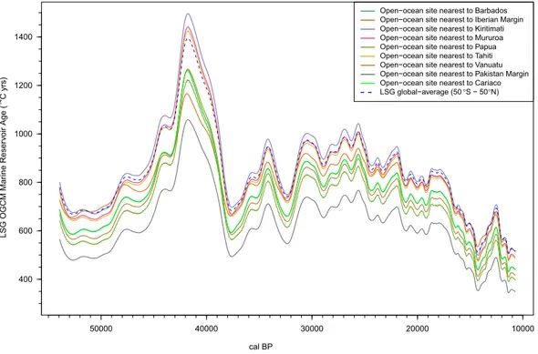
We obtained, under this GS scenario, Hulu-Cave-based MRA estimates for the LSG OGCM open-ocean site closest to the location of each marine dataset (Figure3). These MRA estimates were expected to lack some fine scale features, as the Hulu-Cave-basedΔ14C reconstruction is somewhat smoothed, yet still provide reliable first-order approximations. Since the IntCal20 marine data come from coastal, rather than open-ocean, sites we adjusted the corresponding nearest open-ocean LSG OGCM estimate by application of a constant coastal shift to obtain dataset-specific priors on the MRA for each marine dataset used in IntCal20. This shift aimed to correct for potential coastal effects not accounted for in the LSG OGCM model. Furthermore, to account for the overly smooth nature of these first-order Hulu-Cave-based MRA estimates we allowed additional independent fluctuations around these shifted estimates. Such an approach is analogous to that used to model the speleothem DCFs but, rather than assuming a constant mean, here we use the coastally shifted shape of the LSG OGCM estimates.
Equivalent to the speleothem DCFs, for each of the marine IntCal20 datasets, priors on the magnitude of the coastal shift needed and the size of the independent fluctuations around the
50000 40000 30000 20000 10000
400 600 800 1000 1200 1400
cal BP LSG OGCM Marine Reservoir Age (14C yrs)
Open−ocean site nearest to Barbados Open−ocean site nearest to Iberian Margin Open−ocean site nearest to Kiritimati Open−ocean site nearest to Mururoa Open−ocean site nearest to Papua Open−ocean site nearest to Tahiti Open−ocean site nearest to Vanuatu Open−ocean site nearest to Pakistan Margin Open−ocean site nearest to Cariaco LSG global−average (50°S − 50°N)
Figure 3 First-order regional open-ocean LSG OGCM MRA estimates based upon the LSG’s Glacial Scenario (Butzin et al.2017,2020in this issue) driven by a preliminary estimate of atmospheric Δ14C obtained from the Hulu cave speleothems alone. The plotted values correspond to the LSG site nearest the location of the marine IntCal20 datasets, the MRAs at the open-ocean sites nearest Barbados and Cariaco have almost indistinguishable plotted values. After application of a constant coastal adjustment, these MRAs are used as priors for the marine data in the creation of IntCal20. Note these Hulu-based estimates are intended solely to aid IntCal20 curve construction. In using Hulu Cave to force the LSG, we aim to provide a first-order approximation to the true regional MRAs which, after permitting some further MRA variability, enable the marine data to contribute to the IntCal20 curve. The plotted values are therefore only preliminary coarse approximations of the MRAs for the relevant locations and lack fine-scale structure.
Hulu-Cave-based first-order estimates were obtained from the observed 14C offset between more recent marine samples from that location and overlapping IntCal20 Northern Hemisphere tree-ring data back to ca. 14,190 cal BP. See Heaton et al. (2020b in this issue) for further details and an illustration for Kiritimati. Our prior on the size of coastal shift needed from the open-ocean LSG OGCM estimates ranged from 12 14C yr for Vanuatu corals up to 281 14C yr for Kiritimati. For marine datasets for which we had no observations that overlapped with the Northern Hemisphere tree-ring data, the prior on the coastal shift was chosen to be non-informative while the estimate for the allowable fluctuations was taken from those for sites in the same oceanic region. This non-informative approach permitted us to retain the internal structure in these datasets. With the exception of the Cariaco basin, the resultant coastally shifted prior MRA estimates for each marine dataset were used as inputs for our Bayesian spline method of curve construction. During this process, again analogously to the approach taken to model speleothem DCFs, the constant coastal shift was further updated to resolve potential differences between datasets.
The estimated MRA using the above LSG OGCM based approach was, however, seen to be too high for Cariaco Basin data during the Younger Dryas (ca. 12.9–11.7 cal kBP) which corresponds to Greenland Stadial (GS-1), where it is known to be close to zero from the overlap with the tree rings, and likewise during Heinrich Stadial 1 (ca. 23–12.9 cal kBP, equivalent to GS-2) from comparison with the Hulu Cave data (Hughen and Heaton2020 in this issue). The lack of fit of the LSG OGCM to Cariaco Basin MRA is not surprising given the model resolution of ~380 km compared to the basin size of 160 km by 60 km (Butzin et al. 2020 in this issue) and the shallow sill depth (146 m at present) of the basin (Peterson et al. 2000). Instead, the MRA for Cariaco Basin was modeled as a slowly varying spline and estimated simultaneously to curve construction. Intuitively, this approach enabled the Cariaco data to offer support to the other IntCal20 datasets whereby
14C variations seen in Cariaco data alone were likely to be assigned as MRA changes within the Cariaco basin and not propagate through to the final Intcal20 curve; while 14C features seen not just in Cariaco but also other records would be more likely retained as genuine atmospheric signal (Heaton et al. 2020b in this issue). In IntCal09, the Cariaco Basin data for the Younger Dryas/GS-1 were excluded from consideration because the application of a constant marine reservoir offset caused an offset with the other data and likewise during HS-1/GS-2 in IntCal13 (Reimer et al. 2009, 2013b). With the modeled spline MRA and updated calendar age timescale for the non-varved record, the Cariaco Basin data from the Younger Dryas/GS-1 and HS-1/GS-2 are no longer offset from the rest of the data and are included in IntCal20. The climatic implications of the modeled reservoir age changes for Cariaco Basin data are discussed in Hughen and Heaton (2020in this issue). It should also be noted that the modeled spline MRA for Cariaco Basin beyond the end of the Hulu Cave dataset was extrapolated to 55,000 cal BP to provide the final 1030 cal yr of the IntCal20 curve.
CURVE CONSTRUCTION
After the publication of IntCal13, the IWG determined the necessity of a statistically robust calibration curve construction method that could be run much more quickly than the Random Walk Model (Niu et al.2013), so that different data options could be tested. Several Bayesian and frequentist methods (Kernel density, SIMEX, Bayesian spline) were examined by the IntCal statistics focus group who decided upon a Bayesian spline incorporating calendar age uncertainty (Berry et al. 2002; Heaton et al. 2020b in this issue). The quality of fit of