——————————————————————————————
Hawking Radiation
——————————————————————————————
SEMINAR ON MATHEMATICAL ASPECTS OF THEORETICAL PHYSICS
Klaus Fredenhagen
Mathematical Physics Group Universit¨ at Hamburg
June 2012
Mojtaba Taslimi Tehrani
Advisor:
Thomas-Paul Hack - Christian Pfeifer
1 Introduction
The closest theoretical physics has reached to a quantum gravitational effect is the discovery of black hole radiation. In 1974, Stephen Hawking showed that black holes, which are objects that light cannot escape from and hence classically are at absolute zero, do radiate at temperature
TH= ~c3 8πGM kb
, (1.0.1)
when quantum mechanical effects are taken into account. The presence of both gravitational and quantum mechanical constants reflects the fact that this result should somehow lie in the domain of quantum gravitational regime. In fact, this effect is predicted via studying quantum fields on the curved background of a black hole and the observation that the thermal spectrum of particle creation at infinity lies at temperatureTH. This, of course, is not a quantum theory of gravity since the gravitational field, manifest in curvature of space-time, is kept fixed and its (quantum) dynamics is not intended to be studied. However, this is different from QFT on Minkowski background and hence serves as a semi-classical calculation toward quantum gravitational effects.
In this note, we will review the derivation of Hawking effect for an eternal Schwarzschild black hole in the framework of algebraic quantum field theory. To that end, we will begin with classical description of black holes in section 2, and in section 3 by considering a massless scalar field on the fixed Schwarzschild background, we derive the Hawking radiation.
2 Black Holes in Classical General Relativity
To define a black hole, consider the following preliminary definitions on the space-timeM
• I+(p): (chronological future of a point p∈ M) : the set of events that can be reached by a future directed timelike curve starting fromp;
• I+(S): (chronological future of a subsetS∈ M): I+(S) =∪p∈SI+(p);
• I−(p) andI−(S) (chronological past) are defined analogously;
• I+ (future null infinity) is a null hypersurface which is in fact an idealization of faraway observers who can receive radiation from the isolated gravitating system.
Based on the above definitions, the black hole region,B, of an asymptotically flat space-timeMis defined as:
B=M −I−(I+). (2.0.2)
The horizonHof a black hole is, then, defined as the boundary of B.
2.1 Schwarzschild Black Hole
By applying spherical symmetry to the Einstein’s equations in vacuum, Rµν = 0, one finds the metric describing the space-time outside a spherically symmetric massM
ds2=−
1−2M r
dt2+
1−2M
r −1
dr2+r2dΩ2, (2.1.1) known as the Schwarzschild solution.
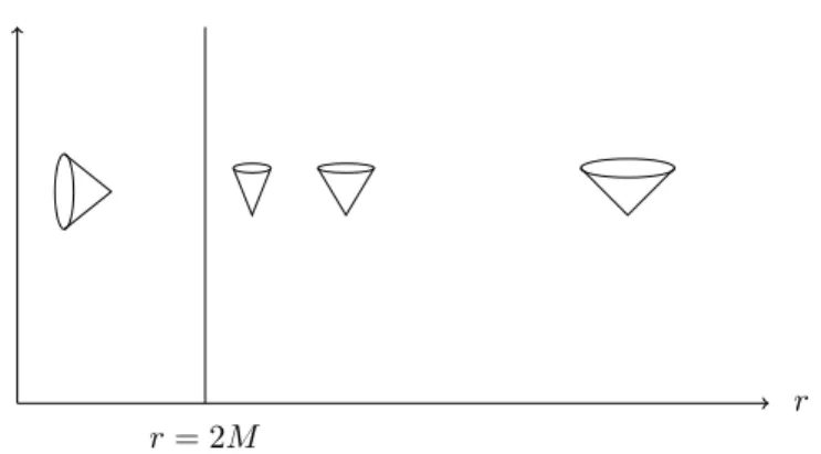
r= 2M
r t
Figure 1: Local light cones in Schwarzschild coordinates
2.1.1 Basic Features
1. Asymptotic flatness: At the limitr→ ∞, the line element 2.1.1 becomes the flat Minkowski line element;
2. Stationary: since it has a timelike Killing vector field,∂t(it does not depend on the coordinate t), it is stationary;
3. Static: since the time-like Killing vector field, ∂t, is orthogonal to the t =const. family of hypersurfaces (there is no cross termdtdxa in the metric), it is static;
4. Kretschmann scalar curvature: RµνρσRµνρσ= 48Mr62;
5. Coordinate singularity: atr= 2M the metric becomes singular which corresponds to a finite value of scalar curvature and hence just a coordinate singularity (see below);
6. Irremovable singularity: at r= 0 the scalar curvature blows up which signals an irremovable singularity;
7. Uniqueness: Brikhoff’s theorem guarantees that the space-time due to a spherically symmetric source is uniquely the Schwarzschild space-time.
2.1.2 Local Causal Structures and Horizon
To study causal structure and consequently to identify the horizon, let’s consider the radial null paths characterized byds2=dΩ2= 0. This leads to the null condition
dt
dr =± r
r−2m (2.1.2)
which determines the local light cones (See figure 1)
At each pointpof space-time, the region within the light cone is causally connected top. As can be seen in the figure, the light cones become closer as one approaches the surfacer= 2M. On the surfacer= 2M, the cone slope blows up and the light cone is totally closed; signals sent from it will remain on the surface and will never reach infinity. In the region within such a surface,r < 2M, the light cone is directed toward the center which means signals never reach the horizon. Such a region defines a black hole: it is the part of space-time excluding the region which is chronologically connected to the future null infinity. The surface r = 2M, the boundary of Schwarzschild black hole, is called horizon i.e. the last surface from which light can scape to future null infinity. On this surfaceg00= 0.
2.1.3 The Kruskal-Szekeres Extension
Let’s consider the 1 + 1 dimensional version of the line element 2.1.1. The Schwarzschild coordinate (t, r) are restricted to the range−∞< t <+∞and r >0. Nevertheless, one may find a suitable coordinate transformation such that not only the fake singularity atr = 2M disappears, but also new coordinates can take all the values including the old coordinates values. This leads us to the concept of extension of a nonsingular region which is defined as finding a non-singular space-time which includes the original space-time as a subset.
To find the maximal extension (the one that cannot be extended further) of Schwarzschild space- time, we perform 4 sets of coordinate transformations.
•First Coordinate Transformations (t, r∗) :
In the first step, we adopt the following coordinates by solving fortthe null condition.
ds2= 0⇒dt=±(1−2M
r )−1dr⇒t=±r∗+const., (2.1.3) wherer∗=r+ln(2Mr −1) with−∞< r∗ <+∞and is known as tortoise coordinate. In terms of (r∗, t):
ds2= (1−2M
r )(−dt2+dr2∗) +r2dΩ2. (2.1.4) Note that the horizon r = 2M corresponds to r∗ → −∞; the whole range of tortoise coordinates cover the region outside the horizon of black hole. The radial light cone equation is obtained by:
ds2= 0 =dΩ2⇒ dt
dr∗ =±1 forr6= 2M, (2.1.5) which means that the light cone has 45◦slope in the whole range of this coordinate.
•Second Coordinate Transformations (u, v) :
Secondly, we consider the following null coordinates defined by:
u=t−r∗;−∞< u <+∞ (2.1.6) and
v=t+r∗;−∞< v <+∞. (2.1.7) In this coordinates, the line element 2.1.1 takes the form
ds2=−2Me−r/2M
r e(v−u)/4Mdudv+r2dΩ2. (2.1.8)
Note that the above line element is regular for all the values ofu, v andr = 2M singularity of the original Schwarzschild coordinates does not appear in this coordinates. Moreover, the light cone is well behaved for allr:
ds2= 0 =dΩ2⇒dudv= 0⇒
u= const.⇔t=r∗+ const.
v= const.⇔t=−r∗+ const. , (2.1.9) they are straight lines in this coordinate which was expected from the fact that (u, v) are null.
Therefore, the singular behavior of the metric 2.1.1 at r = 2M is just an artifact of the special coordinate system chosen and is called acoordinate singularity.
•Third Coordinate Transformation(U, V):
Now, consider U =U(u) and V =V(v) obtained by a transformation of the (u, v) coordinates in the form:
U =−e−u/4M;U <0 (2.1.10)
V =ev/4M;V >0 (2.1.11)
The line element 2.1.1 in this coordinate system takes the form ds2=−32M3
r e−r/2MdU dV +r2dΩ2. (2.1.12) which is obviously well defined atr= 2M. Light cones are again straight lines.
•Forth Coordinate Transformation(T, X):
Finally, the last coordinate transformations, called Kruskal-Szekeres coordinates, take the form:
T =1
2(U +V);−∞< T <+∞ (2.1.13) X =1
2(U−V);−∞< X <+∞, (2.1.14) and leads to the line element
ds2= 32M3
r e−r/2M(−dT2+dX2) +r2dΩ2. (2.1.15) The Schwarzschild coordinates can be expressed in terms of Kruskal-Szekerz coordinates as:
( r
2M −1)er/2M =X2−T2, (2.1.16)
t= 4M tanh−1(T
X). (2.1.17)
The advantage of this coordinate system is that the light cone has every where 45◦ slopes and is well defined for all values ofr:
ds2= 0 =dΩ2⇒ dT
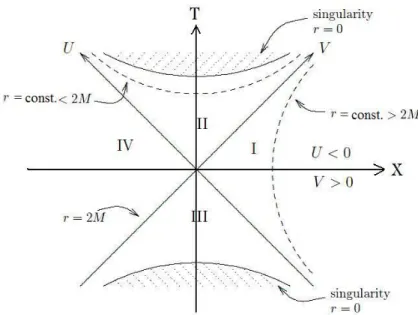
dX =±1 for all r. (2.1.18) The following features of the maximally extended space-time can be read easily from the 2 dimen- sional figure 2 :
• Region I: the range of original Schwarzschild radial coordinater >0 corresponds toX2−T2>
0, which sits in the region I of the extended space-time and is in fact the exterior gravitational field of a spherical body,
• Ther= 0 singularity corresponds toX=±(T2−1)1/2; it lies at future of II and past of III,
• Region II (Black Hole): this region corresponds to the r < 2M portion of Schwarzschild coordinates,
• X = ±T Horizon are straight line representing null geodesics which serve as the boundry between black hole and outside,
Figure 2: Extended Schwarzschild space-time in 1+1 dimensional Kruskal-Szekeres coordinates.
Each point is understood as a 2-sphere.
• Radially infalling observers in I will cross X =T and fall into II. However, they can never scape from II; within a finite proper time will fall into singularity,
• Region III(White Hole): this region has the time-reversed properties of II; every observer must have originated from −(T2−1)1/2 and must leave III within a finite time,
• Region IV: identical properties to I; another asymptotically flat space-time lying insider = 2M,
• Regions I and IV cannot communicate; light signals from I are swallowed by singularity and never reaches IV.
3 Hawking Radiation
3.1 Physical Motivation
The Hawking radiation was originally discovered for collapsing stars which end up at black holes.
However, what we are considering here is an eternal black hole (one that has always existed) which is closely related to the Unruh effect. In order to see the similarity and gain some motivation for the calculations of black hole radiation, we review briefly the Unruh effect.
3.1.1 Review of Unruh Effect
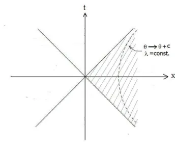
Consider the Rindler space-time characterized by the line element
ds2=a2e2λ(−dθ2+dλ2). (3.1.1) The coordinates (θ, λ) can be obtained from the usual Minkowski coordinates (t, x) by a transfor- mation of the form
Figure 3: Rindler space-time as the wedge |t|< xof the Minkowski space-time.
θ=1
atanh−1(t
x) (3.1.2)
λ= 1
2aln(x2−t2). (3.1.3)
It means that the Rindler space-time is, in fact, the wedge|t|< xof the Minkowski space-time. The factora, which from the above relations becomea= x21−t2, corresponds to the uniform acceleration of an observer in (t, x).
The Unruh effect amounts to different interpretations of a quantum state by distinct observer.
Consider two sets of observers in Minkowski space-time:
1. Inertial observers : not influenced under any external force and naturally use the standard Minkowski coordinates (t, x). Their world lines are straight lines within the causal null cone.
2. Uniformly accelerated observer: have uniform acceleration a= x2−t1 2 as seen by the inertial observers. Therefore, their world lines follow along the curves of constant acceleration which correspond to λ=const.in coordinates (θ, λ). Since the Rindler wedge lies out side the light cone, such accelerated observers are causally disconnected from the inertial observes.
The Unruh effect basically states that:
The uniformly accelerated observer “sees” the state of a quantum field, expressed by a 2-point functionω2(λ, θ, λ0, θ0), as a KMS state ω2β(λ, θ, λ0, θ0) = ω2β(λ0, θ0 +iβ, λ, θ) at temperature T =
1
β = 2πa , while the inertial observer’s 2-point function ω(x, t, x0, t0) does not have such a thermal behavior.
3.1.2 Analogy with Eternal Black Holes
The obvious similarities can be seen by comparing the diagrams of Kruskal-Szekeres and Rindler space-times. First, note that the region out of horizon of a black hole corresponds to the wedge
|T| < X (region I) in Kruskal-Szekeres space-time just as the Rindler is the wedge |t| < x in Minkowski space-time. Second, the orbits of time translation,t→t+c0, in Schwarzschild coordinates (ther=const. >2M curves) are one branch of hyperbola in region I, just like the orbits of time
translation in Rindler coordinates, θ → θ+c, are one branch of hyperbola in the Rindler wedge.
Moreover, notice the similarity between coordinate transformations t= 4M tanh−1(T
X), (3.1.4)
r∗= 2M ln(X2−T2), (3.1.5)
and 3.1.2, 3.1.3. These similarities suggest to define two sets of observers in the curved space-time of black hole in analogy to those we defined in the flat Minkowski space-time:
1. Freely falling observer: not influenced under any external force and are freely falling in the gravitational field. They naturally use the Kruskal-Szekeres coordinates (T, X);
2. Static observers: are kept at somer=const. >2M. Their world lines follow along the curves of Schwarzschild time translation. They lie outside the horizon and are causally disconnected from the region inside the black hole. They use the coordinates (r∗, t).
Based on the above analogy, one expect to observe an effect similar to Unruh effect: the static observer would see some “thermal effect”, while the freely falling observer would not. Furthermore, comparing 3.1.4, 3.1.5 with 3.1.2, 3.1.3, one can identifya=4M1 and anticipate that such a thermal effect would occur at temperatureT = 2πa = 8πM1 . The Hawking radiation effect basically states that:
The static observer “sees” the correlation functionω(t, r∗, t0, r0∗), between horizon and the region outside black hole as a KMS (thermal) state at temperatureT = β1 = 2πa , while the freely falling observer does not detect such a thermal behavior.
3.2 Mathematical Derivation
In this section, we investigate the anticipation of the last section in the following steps:
1. consider a free massless scalar field on the background of a Schwarzschild black hole;
2. construct a 2-point functionω2β(t, r∗, t0, r∗0) for the static observer satisfying (i) the K-G equa- tion in (r∗, t) coordinates (ii) the positivity conditionω2β(f∗, f)≥0, (iii) the KMS condition for some inverse tempratureβ;
3. sinceω2β turns out to be singular, calculate∂T∂T0ωβ2(r∗;r∗0) which is finite;
4. study∂T∂T0ωβ2(−∞;r0∗): the correlation between horizon and the region outside of black hole;
5. observe that such a correlation is well defined only for temperatureT = 8πM1 .
A massless free Klein-Gordon field on a globally hyperbolic space-time satisfies the equation:
gφ= 0, (3.2.1)
where
g≡ 5µ5µ =|g|−12∂µgµν|g|12∂ν. (3.2.2) In tortoise coordinates, the above wave operator takes the form:
g= (1−2M r )−1
∂t2−1 r∂r2∗r
+ (2M
r3 −4S2
r2 ). (3.2.3)
where 4S2 is the Laplace operator on the two sphere. We now consider the spatial part of this operator
A=−1
r∂r2∗r+ (1−2M
r )−1(2M r3 −4S2
r2 ), (3.2.4)
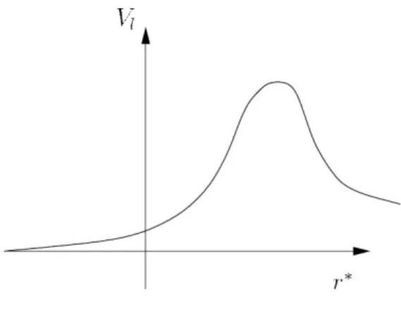
Figure 4: The potentialVl(r∗)
and search for eigenfunctions of the form Φ(r∗, θ, φ) = P
lmf(r∗)Ylm(θ, φ) with Ylm(θ, φ) being spherical harmonics and so eigenfunctions of4S2. Hence,Abecomes
A=−1
r∂2r∗r+Vl(r), (3.2.5)
with
Vl(r) = (1−2M r )−1
l(l+ 1) r2 +2M
r3
(3.2.6) This operator describes the movement of a quantum mechanical particle in the potential Vl(r∗).
The potential decays forr∗→ ∞(corresponding to r= 2M) exponentially and forr∗→ ∞like r12
∗
and reaches a finite maximum at some value ofr(see figure 4). Since we are interested in thermal effects near horizon, we can neglect the potential term for the time being and proceed with finding the 2-point function of the operatorA=−1r∂r2∗r.
The 2-point function takes the form:
ω2(t, r∗;t0, r∗0) = 1 2√ A
exp
−i√
A(t−t0) 1−e−β
√
A +
exp i√
A(t−t0) eβ
√ A−1
(r∗, r∗0) := f(√
A)(r∗, r∗0). (3.2.7)
We verify this by showing that it satisfies the Klein-Gordon equation 3.2.1. Note that a state ω is a distribution and soω2(t, r∗;t0, r0∗) must be seen as the kernel of a distribution:
gω2(f, g) = Z
dr∗d4r0∗gω2(t, r∗;t0, r0∗)f(r∗)g(r0∗)
= Z
dr∗d4r0∗(1−2M
r )−1 ∂t2−A
ω2(t, r∗;t0, r∗0)f(r∗)g(r∗0)
= Z
dr∗d4r0∗(1−2M
r )−1(A−A)ω2(t, r∗;t0, r0∗)f(r∗)g(r∗0)
= 0. (3.2.8)
To be a state,ω must be positive as well. We check that after writing the mode decomposition of ω2.
The OperatorAacting on a functionf ∈C0∞(R×S2)∈L2(R×S2, r2sinθdr∗dθdφ) takes the form:
Af=−1
r∂r2∗(rf) =−∂r2∗f−f
r∂r2∗r−2
r(∂r∗r)(∂r∗f). (3.2.9) However, we can make use of a transformation of the form:
U :L2(R×S2, r2sinθdr∗dθdφ)→L2(R×S2, sinθdr∗dθdφ),
f 7−→f r, (3.2.10)
and observe thatA acting onf rwould take the simpler form:
A0 =U AU−1=∂r2∗. (3.2.11)
Therefore, it would be more convinient to work withA0 instead ofA.
Now, letφ~p∈ Hbe an eigenvector ofA0:
A0φ~p=|~p|2φ~p. (3.2.12)
Thenφ~p will take the form
φ~p=ei~p. ~r∗. (3.2.13)
SinceA0 is positive (|~p|2>0) and diagonal onφ~p, the operator
√
A0 can be defined: it has the same eigenvectors asA0 with the square root of its eigenvalues:
√
A0φ~p=|~p|φ~p. (3.2.14)
SinceA0 is essentially self adjoint, we can write the above expression forω2(t, r∗;t0, r0∗) as a mode decomposition using spectral theorem according to which, a functiong of a self-adjoint operatorO (withOΦk =oΦk) acting on an elementh∈ Hcan be written as
g(O)h= Z
f(o(k))Φk(Φk, h)dµk. (3.2.15) For the case off(√
A0) defined by 3.2.7 it leas to:
f(
√
A0)h(r∗) = Z
f(p)φ~p(φ~p, h)dµp~ (3.2.16)
= Z
f(p)ei~p.~r∗d~p Z
e−i~p.~r∗0h(r∗0)dr0∗ (3.2.17)
= Z
d~pdr0∗f(p)e−i~p.(~r∗0−~r∗)h(r∗) (3.2.18) Thus,f(√
A0)(r∗, r0∗) =R
d~pf(p)e−i~p.(~r∗0−r∗)~ can be seen as the kernel of a distribution. This way, we can express the correlation function 3.2.7 as:
ω2(t, r∗;t0, r∗0)
= (2π)−1 Z
dp 1 2p
e−ip(t−t
0)
1−e−βp +eip(t−t
0)
eβp−1
! e−ip(r
0
∗−r∗)
(3.2.19)
Before discussing the thermal nature of such a state, let us verify that it is positive.
ω2(f∗, f)
= (2π)−1 Z
dp 1 2p
e−ip(t−t
0)
1−e−βp +eip(t−t
0)
eβp−1
! e−ip(r
0
∗−r∗)
= (2π)−1 Z
d4xd4x0dp 1 2p
e−ip(t−t
0)
1−e−βp +eip(t−t
0)
eβp−1
!
×e−ip(r
0
∗−r∗)f∗(x)f∗(x0)
= (2π)−1 Z
dp 1
2p|cp|2 (3.2.20)
wherecp=R
d4xexp(−ip
µ(t,r∗)µ)
1−e−βp +exp(ipeβpµ(t,r−1∗)µ)
f(x). Hence,ω2 is positive. Moreover, it is easy to see that it satisfies the KMS condition:
ωβ2(t+iβ, r∗;t0, r0∗)
= (2π)−1 Z
dp 1 2p
e−ip((t+iβ)−t0)
1−e−βp +eip((t+iβ)−t0)
eβp−1
! e−ip(r
0
∗−r∗)
= (2π)−1 Z
dp 1 2p
eβpe−ip(t−t
0)
1−e−βp +e−βpeip(t−t
0)
eβp−1
! e−ip(r
0
∗−r∗)
= (2π)−1 Z
dp 1 2p
eip(t−t
0)
1−e−βp +e−ip(t−t
0)
eβp−1
! eip(r
0
∗−r∗)
= ω2β(t0, r0∗;t, r∗).
The state ω2β is, however, not well defined; it is singular at p = 0. Nevertheless, we can show that its time derivative is well defined which would lead to the conclusion that the state ω2β is well defined on the sub-algebra of the time derivative of the fields, which are again fields (recall that a stateω in the algebraic formulation of QFT is a functional over the fieldsφ, φ0: ω(φ, φ0) = Rdxdx0ω(x, x0)φφ0. Thus, after integration by part, for the time derivative of a state we can write Rdxdx0ω(x, x0)∂tφ, ∂t0φ0 =ω(∂tφ, ∂t0φ0), which can be seen as another state on ∂tφ,∂t0φ0).
Taking the derivative ofωβ2(t, r∗;t0, r0∗) with respect tot0 andt att0 =t= 0 we get:
∂t∂t0ω2(t, r∗;t0, r0∗)
= (4π)−1 Z
dpp2 2p
e−ip(t−t
0)
1−e−βp +eip(t−t
0)
eβp−1
!
×e−ip(r
0
∗−r∗) (3.2.21)
∂t∂t0ω2(t, r∗;t0, r0∗)|t=t0=0
= (4π)−1 Z
dpp 1
1−e−βp + 1 eβp−1
e−ip(r
0
∗−r∗)
= (4π)−1 Z
dppcoth(βp 2 )e−ip(r
0
∗−r∗)
. (3.2.22)
It has poles atβp= 2πniforn∈Nand can be evaluated using the residue theorem:
Res
pcoshβp/2
sinhβp/2e−ip.(r∗0−r∗)
p=2πniβ = 2
βpcosh βp/2 cosh βp/2e−ip(r
0
∗−r∗) p=2πniβ
= 2πni β2 e2πnβ .(r
0
∗−r∗)
(3.2.23)
∂t∂t0ω2β(t, r∗;t0, r0∗)|t=t0=0 = (4π)−12πi
∞
X
n=0
res(2πni/β)
= π
β2
∞
X
n=0
ne2πnβ (r∗−r
0
∗)
= π
β2sinh−2 π
β(r∗−r0∗)
. (3.2.24)
To make the final conclusion (correlation between horizon and outside) , it would be more transparent if we express the derivative ofω2β with respect to the Kruskal-Szekeres time coordinateT atT = 0 (on the horizon). To that end, we use the chain rule:
∂
∂T
∂
∂T0 = ∂t
∂T
∂
∂t
∂t0
∂T0
∂
∂t0
!
. (3.2.25)
From 2.1.17 we have:
∂t
∂T = 4M X
X2−T2, and ∂t0
∂T0 = 4M X
X2−T02 (3.2.26)
Therefore,
∂
∂T
∂
∂T0|T=T0=0= (4M)2XX0 ∂
∂t
∂
∂t0|t=t0=0. (3.2.27) ExpressingX in terms ofr∗ using relations 2.1.10 and 2.1.11 we get
∂
∂T
∂
∂T0|T=T0=0= (4M)2e−(r∗+r
0
∗)/4M ∂
∂t
∂
∂t0|t=t0=0. (3.2.28) Therefore, the time derivative of the correlation function 3.2.24 expressed with respect to Kruskal- Szekeres time takes the form :
∂T∂T0ωβ2(r∗;r0∗) = α2e−(r∗+r
0
∗)/4Msinh−2 π
β(r∗−r0∗)
= α2 e−(r∗+r
0
∗)/4M
e2πβ(r∗−r0∗)+e2πβ(r∗−r0∗)−2
= α2n e(β(r∗+r
0
∗)+8πM(r∗−r∗0))/4M β+e(β(r∗+r
0
∗)−8πM(r∗−r∗0))/4M β
−2e(r∗+r
0
∗)/4Mo−1
= α2n
e((β−8πM)r
0
∗+(β+8πM)r∗)/4M β+e((β+8πM)r
0
∗+(β−8πM)r∗)/4M β
−2e(r∗+r
0
∗)/4Mo−1
(3.2.29)
whereα2= (4M)β22π.
We are interested in correlations between horizon (r∗ → −∞) and an arbitraryr0∗ outside the horizon. Hence, our final task is now to inquire under which condition ∂T∂T0ωβ2(−∞;r0∗) is well defined. To that end, lets factor oute−(β−8πM)r
0
∗/4M β in 3.2.29 and write it as:
∂T∂T0ω2β(r∗;r0∗) = α2e−(β−8πM)r∗/4M β
e(β+8πM)r0∗/4M β+e((16πM)r∗+(β−8πM)r∗0)/4M β−2e(βr∗0+8πM r∗)/4M β
(3.2.30) It is clear that for r∗ → −∞ the nominator blows up while the denominator remains finite. The only way to keep the nominator finite is to setβ= 8πM which leads to:
∂T∂T0ωβ=8πM2 (−∞;r0∗) = 1
4Me−2M1 r
0
∗. (3.2.31)
Note that correlation between horizon and the region outside the black hole vanishes asymptotically asr0∗→ ∞, and diverges as one reaches the horizonr∗0 → −∞(such a divergence is of course of the familiar type of divergences one normally encounters in QFT: the correlation function between the same points corresponds to the product of two fields at the same point and hence is ill-defined).
To sum up, we have shown that for a static observer the correlation function between horizon and the region outside the horizon is a thermal state which is well-defined uniquely for T = β1 =
1
8πM ≡TH. This can be interpreted as:
An observer kept at constant r outside the black hole receives thermal radiation coming from the horizon; black holes radiate atTH.
Note that in the Unruh effect, the temperature depends on acceleration T = 2πa; different uni- formly accelerated observers following along distinct λ = const. hyperbolas experience different temperatures. The temperature obtained above,T = 8πM1 , is in fact the temperature measured by a static observer near infinity. However, the locally measured temperature of the Hawking radiation follows the Tolman law, according to which the temperatureT of a thermodynamical system as seen by an observer in the gravitational field who is following an orbit of a Killing vector fieldξµappears as T(−ξµξµ)−1/2. This means that the temperature of the radiating black hole for distinct static observers following the different orbits of a Killing vector fieldξµ is:
TH = 1
8πM(−ξµξµ)1/2. (3.2.32)
References
[1] R. M. Wald, General Relativity, The University of Chicago Press, Chicago 1989.
[2] P. K. Towsend, Black Holes, 1997, arXiv:gr-qc/9707012v1.
[3] K. Fredenhagen, Quantenfeldtheorie in gekrummte Raumzeit.