Article
Unmanned Aerial Systems for Investigating the Polar Atmospheric Boundary Layer—Technical Challenges and Examples of Applications
Astrid Lampert1 , Barbara Altstädter1 , Konrad Bärfuss1 , Lutz Bretschneider1, Jesper Sandgaard1 , Janosch Michaelis2 , Lennart Lobitz1, Magnus Asmussen1 , Ellen Damm2 , Ralf Käthner3, Thomas Krüger1 , Christof Lüpkes2 , Stefan Nowak1, Alexander Peuker1, Thomas Rausch1 , Fabian Reiser4 , Andreas Scholtz1,†,
Denis Sotomayor Zakharov5, Dominik Gaus5, Stephan Bansmer5, Birgit Wehner3and Falk Pätzold1,*
1 Institute of Flight Guidance, Technische Universität Braunschweig, 38106 Braunschweig, Germany;
Astrid.Lampert@tu-braunschweig.de (A.L.); b.altstaedter@tu-braunschweig.de (B.A.);
k.baerfuss@tu-braunschweig.de (K.B.); l.bretschneider@tu-braunschweig.de (L.B.);
j.sandgaard@tu-braunschweig.de (J.S.); l.lobitz@tu-braunschweig.de (L.L.);
m.asmussen@tu-braunschweig.de (M.A.); t.krueger@leichtwerk-research.de (T.K.);
stefan.nowak@tu-braunschweig.de (S.N.); a.peuker@tu-braunschweig.de (A.P.);
Thomas.Rausch@tu-braunschweig.de (T.R.); ingenieurbuero.scholtz@gmx.de (A.S.)
2 Alfred Wegener Institute, Helmholtz Centre for Polar and Marine Research, 27570 Bremerhaven, Germany;
Janosch.Michaelis@awi.de (J.M.); Ellen.Damm@awi.de (E.D.); Christof.Luepkes@awi.de (C.L.)
3 Institute of Tropospheric Research, 04318 Leipzig, Germany; kaethner@tropos.de (R.K.);
birgit@tropos.de (B.W.)
4 Institute of Environmental Meteorology, University of Trier, 54296 Trier, Germany; reiser@uni-trier.de
5 Institute of Fluid Mechanics, Technische Universität Braunschweig, 38106 Braunschweig, Germany;
d.sotomayor-zakharov@tu-braunschweig.de (D.S.Z.); d.gaus@tu-braunschweig.de (D.G.);
s.bansmer@tu-braunschweig.de (S.B.)
* Correspondence: f.paetzold@tu-braunschweig.de; Tel.: +49-531-391-9885
† Current address: Butzbacherstr, 8 35510 Butzbach/Nieder-Weisel, Germany.
Received: 21 February 2020; Accepted: 4 April 2020; Published: 21 April 2020
Abstract:Unmanned aerial systems (UAS) fill a gap in high-resolution observations of meteorological parameters on small scales in the atmospheric boundary layer (ABL). Especially in the remote polar areas, there is a strong need for such detailed observations with different research foci. In this study, three systems are presented which have been adapted to the particular needs for operating in harsh polar environments: The fixed-wing aircraft M2AV with a mass of 6 kg, the quadrocopter ALICE with a mass of 19 kg, and the fixed-wing aircraft ALADINA with a mass of almost 25 kg. For all three systems, their particular modifications for polar operations are documented, in particular the insulation and heating requirements for low temperatures. Each system has completed meteorological observations under challenging conditions, including take-off and landing on the ice surface, low temperatures (down to −28◦C), icing, and, for the quadrocopter, under the impact of the rotor downwash. The influence on the measured parameters is addressed here in the form of numerical simulations and spectral data analysis. Furthermore, results from several case studies are discussed:
With the M2AV, low-level flights above leads in Antarctic sea ice were performed to study the impact of areas of open water within ice surfaces on the ABL, and a comparison with simulations was performed. ALICE was used to study the small-scale structure and short-term variability of the ABL during a cruise of RVPolarsternto the 79◦N glacier in Greenland. With ALADINA, aerosol measurements of different size classes were performed in Ny-Ålesund, Svalbard, in highly complex terrain. In particular, very small, freshly formed particles are difficult to monitor and require the active control of temperature inside the instruments. The main aim of the article is to demonstrate the
Atmosphere2020,11, 416; doi:10.3390/atmos11040416 www.mdpi.com/journal/atmosphere
potential of UAS for ABL studies in polar environments, and to provide practical advice for future research activities with similar systems.
Keywords: unmanned aerial systems; polar atmosphere; meteorological sensors; atmospheric boundary layer
1. Introduction
Unmanned aerial systems (UAS) have been deployed for meteorological measurements for many decades, dating back to first applications in the 1970s [1]. However, due to the quick development of miniaturized sensors for controlling unmanned aircraft (global navigation satellite systems—GNSS, inertial measurement units—IMU), enhanced by the demands of mobile phone, automotive, and automation industries, UAS have experienced a high increase in usage and a broad range of applications in recent years. In atmospheric sciences, they represent new opportunities for filling the gap of flexible high-resolution measurements on small scales in the atmospheric boundary layer and in particular close to the ground, which cannot be achieved by manned aircraft with a certain minimum flight altitude and much higher cruising speed, or by remote sensing applications with much coarser spatial resolution [2]. Large unmanned systems of the size and weight class similar to manned aircraft, e.g., the Arctic dropsonde campaigns with the Global Hawk [3], are not considered here.
As an example, the investigation of the impact of open water areas within sea ice on the ABL is only possible during flights at very low altitudes. The cold surface temperatures of the ice in winter down to−20 to−30◦C are in strong contrast to the surface water temperatures at the salinity-determined freezing point, about−1.8◦C [4]. For situations of cracks and leads in sea ice, the strong thermal contrasts on small scales may alter the atmospheric temperature [5]. The polynyas are a strong source of sensible and latent heat [6].
In polar areas, the operation of UAS may on the one hand be less restrictive, as risks of ground damage are lower than for operations close to densely populated areas. On the other hand, the harsh environmental conditions pose challenges for operations, sensors, and crew. Furthermore, environmental protection is an important issue, with strict regulations concerning waste management in particular in the Antarctic.
The low temperatures do not only reduce battery capacities for electric propulsion. For many sensors, a thermal insulation of the payload has to be applied, or at least temperature dependence has to be corrected in a post-processing quality control procedure. Take-off and landing require different concepts, as ice surfaces provide less friction, and materials like rubber for bungee starts lose elasticity.
For flights in polar areas, icing turned out to be a major challenge. Methods have been proposed to estimate the icing potential based on the real-time data of temperature and relative humidity, using threshold criteria and the second derivative of the parameters to identify clouds, similar to criteria for icing forecast [7]. Avoiding zones with icing potential and confirming that icing cannot occur by monitoring temperature and relative humidity in real-time is another method of protecting UAS [8]. Systems were modified with monitoring, anti-icing and de-icing devices [9]. This included icing observation by real-time video transmission of ice accretion, and piezoelectric detection of icing.
In addition to carefully avoiding icing zones and heating the pitot tube, anti-icing coatings on the wings and propellers were implemented to reduce icing problems [9].
Using UAS in the Arctic to monitor the surface properties, e.g., sea ice, and gain insight into meteorological processes by measuring meteorological parameters has been addressed by the Aerosonde applications, with an endurance of more than 24 h with a combustion engine [9]. The highly variable vertical aerosol distribution above Svalbard has been observed by different measurement systems (condensation particle counter, chemical sampler, absorption photometer, e.g., [8,10]). UAS have further been used in the polar areas for a multitude of different purposes related to Earth
observation, e.g., plant mapping [11] and tundra monitoring [12], data transmitting from under-ice vehicles [13], monitoring of glacier melt [14], and snow depth mapping [15].
The main purpose of this work is a presentation of technical solutions for three different UAS that have been proven reliable during polar applications and of illustrative results obtained at different sites in the polar regions. The intention is not to provide a validation of the airborne sensors against other instrumentation, which has been published already for each system. The fixed-wing UAS M2AV and ALADINA have been developed originally for operation in temperate climate zones but were modified for the polar conditions. In particular for ALADINA, the aerosol payload requires certain operation temperatures, and the payload compartment was insulated and tempered actively. The characterization and control of condensation particle counters for reliably measuring ultrafine particles in polar environments onboard an airborne system are presented. The quadrocopter ALICE has been designed for polar missions, and every component was tested in a climate chamber independently. None of these systems were designed to be operated in clouds (and precipitation), as current legislation did not allow operations beyond visual line-of-sight (BVLOS).
Furthermore, case studies of atmospheric research are provided, showing the large potential of UAS for polar research, and the research gaps that can be addressed with these systems. The case studies include the observations of turbulent properties above leads in Antarctic sea ice, the quick transformation of air mass properties above Arctic sea ice, and the vertical aerosol distribution in Svalbard.
2. Unmanned Systems and Polar Operations
In this section, three different types of UAS of the Institute of Flight Guidance, TU Braunschweig, with different meteorological payloads are introduced. They were applied in the polar areas in the time period 2013 to 2018 [16–18]. Each system is presented in the following, and a quick overview of the performed polar campaigns is provided, summarized in Table1.
Table 1. Overview of the systems, instrumentation and measurement campaigns presented in the article.~vrepresents the wind vector, “T” stands for air temperature, “hum” humidity, “rad” radiation,
“air samp” air sampling and “surf T” is surface temperature.
Name and System Sensors Polar Campaign Case Study
M2AV (fixed-wing, Section2.1, Section3.1) ~v, T, hum (Section2.1) Weddell Sea 2013 icing (Section3.5), leads (Section4.1), ALICE (quadrocopter, Section2.2, Section3.2) T, hum, surf T, rad, air samp (Section3.4) Greenland Sea 2017 T variability (Section4.2), ALADINA (fixed-wing, Section2.3, Section3.1, Section3.3) ~v, T, hum, surf T, rad, aerosol (Section4.3) Svalbard 2018 aerosol variability (Section4.4)
2.1. M2AV
The M2AV (Meteorological Mini Aerial Vehicle) is a fixed-wing aircraft of 2 m wingspan and a take-off mass of 6 kg (see Figure1). It has been developed at the Institute of Aerospace Engineering, TU Braunschweig. It is powered electrically with twin engines, leaving the nose for meteorological sensors and data acquisition. The typical cruising speed is 22 m s−1, and the flight endurance is around 50 min.
The M2AV was the first UAS equipped with a miniaturized five-hole probe and GNSS/IMU to derive the 3D wind speed [19,20]. The method is based on the vector subtraction of the true air speed and the ground speed and is described in detail in [21,22]. The M2AV is also instrumented with a standard Vaisala HMP50 temperature and humidity sensor (Vaisala, Finland), and a fast fine-wire sensor for deriving the temperature with high temporal resolution. The system has been characterized and compared extensively to well-established measurement techniques like radiosondes, meteorological towers, and remote sensing systems like profilers [23]. Turbulence properties have been compared to a tethered balloon system [24] and to tower measurements and numerical simulations [25]. The M2AV was the base for the development of further UAS, like ALADINA (see Section2.3) and the UAS MASC (Multi-Purpose Airborne Sensor Carrier) of the University of Tübingen [26,27]. To date, there is a large number of other UAS with turbulence probe, e.g., [28,29].
The M2AV was operated on the research vessel (RV)Polarstern during the winter expedition PS81 ANT-XXIX/6 in the Antarctic Weddell Sea from 8 June 2013 to 12 August 2013. Altogether, 11 flights were performed up to an altitude of 1400 m with a total flight time of around 6 h. In order to estimate turbulent properties, horizontal legs with 2–4 km length close to the ice surface were chosen in the study.
Figure 1.The M2AV in front of the RVPolarsternin the Weddell Sea on 11 July 2013. Photo: Andreas Scholtz, TU Braunschweig.
2.2. ALICE
The development of the quadrocopter ALICE (Airborne tool for methane isotopic composition and polar meteorological experiments) was motivated by the idea to perform measurements of temperature, humidity, upwelling and downwelling solar irradiance and surface temperature, and to take air samples for subsequent laboratory analyses [30]. The aim was to apply the system in the polar environment, and in particular from locations of small space, like the RVPolarstern. Therefore, from the beginning, ALICE was designed in a way to be handled easily and flexibly under cold conditions.
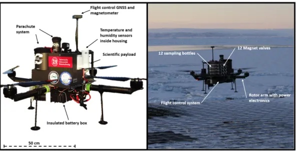
The main construction consists of a central plate and four removable arms with motors T-Motor U11 120 KV and propeller blades T-Motor 26× 8.5 CF (T-Motor, Nanchang, China). They are quickly connected and disconnected mechanically, including electric contacts. The central plate contains the LiPo batteries, the PixHawk autopilot system, and several sensors described below. Flights have only been performed in line of sight, and no de-icing systems were implemented. For safety reasons, an emergency parachute is included, which can be triggered by a separate telemetry link via remote control (Figure2).
The typical mission profile of ALICE is a vertical climb up to 1000 m and then a descent.
The telemetry data transmission allows for identifying layers of interest, e.g., a temperature inversion, and to decide on altitudes for the air samples based on the real-time atmospheric data [30]. ALICE has been operated up to a wind speed of 70 km h−1, and climbing was still possible with a vertical speed of 8 m s−1.
The sensors include several different thermometers, a HMP110 (Vaisala, Finland), a digital sensor TSYS01 (Innovative Sensor Technology, IST, Switzerland), and two platinum fine-wire sensors manufactured at the Institute of Flight Guidance, TU Braunschweig, described in [21]. The water vapor mixing ratio is measured with the capacitive sensor HMP110 as well, and the Rapid P14 of IST (Switzerland). The temperature and humidity sensors are integrated in a housing which protects against solar irradiance and heat of the motors (Figure2). A static and dynamic pressure sensor (AMS 5812, AMSYS, Germany) are integrated in the housing to derive the barometric altitude and air density and to estimate the vertical flow speed through the housing. Furthermore, two pyranometers (ML-02
Si-Pyranometer, EKO, the Netherlands) were integrated looking in nadir and zenith direction as an indicator of cloud and sea ice conditions. An infrared thermometer MLX90614 (Melexis, Belgium) in nadir looking configuration is included. Twelve evacuated glass bottles are integrated for air sampling.
They can be opened by electromagnetic valves triggered by the autopilot at predefined altitudes, or manually by the operator at the ground station. The working principle has been demonstrated in [17,30], but no air samples are available for the campaign presented here.
Figure 2.Quadrocopter ALICE with its components and sensors. The white housing containing the meteorological sensors is visible in the left figure.
An estimation of the flow induced by the rotor blades during different flight states has been presented in [30].
All components were tested in a climate chamber down to−40◦C. Additionally, vibration spectra recorded during test flights were applied during the chamber measurements by a shaker of type Mini Shaker 4810 (Brüel and Kjaer, Denmark). The flow and impact of rotors on the measurements is analyzed in detail in Section3.4. ALICE was deployed during thePolarsternexpedition PS109 (ARK-XXXI/4) to the northeast Greenland Sea from 16 September to 14 October 2017. Overall, eight measurement flights were performed up to an altitude of 1000 m with a total flight time of 1 h 7 min.
2.3. ALADINA
The development of ALADINA (Application of Light-Weight Aircraft for Detecting in-situ Aerosol) was based on the unmanned system “Carolo P360” and the motivation to include additional payload on a fixed-wing meteorological UAS with the main focus on boundary layer aerosol particles [31]. The system has a wing span of 3.6 m and a maximum take-off mass of close to 25 kg, including the payload with a mass of 4.5 kg. It is a pusher configuration with the propeller at the back, to avoid disturbance of the flow at the nose where the atmospheric measurement technique is integrated in a payload bay. The aircraft is powered by a 3.8 kW electric motor which provides sufficient thrust for agile maneuvering, and it is not polluting the aerosol measurements with any combustion products. For a designated flight time of up to 40 min, the main batteries capacity is chosen to hold 1 kWh of energy. The cruising speed is 28 m s−1, and a safe operation is guaranteed for wind speed less than 15 m s−1. To ensure a maximum of safety, all avionics (such as the flight guidance and navigation system) run on separate and redundant power supplies. The UAS was controlled with the autopilot Pixhawk 2.1 Cube (open-hardware project).
ALADINA was deployed during a measurement campaign in Ny-Ålesund, Svalbard.
As Ny-Ålesund is a radio silent zone and the use of frequencies above 2 GHz is not allowed, the telemetry system was modified to use only the radio frequencies of 433 and 868 MHz.
The meteorological payload contained in the nose was first adapted from the M2AV payload.
Additionally, aerosol instrumentation was implemented, consisting of two condensation particle counters (CPCs, model 3007, TSI Inc., Shoreview, MN, USA) to record the number concentration of aerosol particles. These CPCs were modified to achieve different lower detection limits. More details about the modification and the resulting measurement range can be found in Section4.3.
In addition, an optical particle counter (model GT-526S, Met One Instruments Inc., Grants Pass, OR, USA) was integrated for information on aerosol particle number concentration in the size range from 390 nm to 10µm in six size classes [31,32]. The airborne instrumentation shows good agreement with ground-based measurements [33]. The payload of ALADINA was modified and improved continuously based on the experience during field campaigns and data analysis. To obtain information on the current cloud situation, upward and downward looking pyranometers were included [21].
Furthermore, an aethalometer (AE51, Envilyse, Essen, Germany) was integrated to measure the black carbon mass concentration [34].
During the campaign in Svalbard from 24 April to 25 May 2018, 50 measurement flights were carried out with a total flight time of 30 h and 220 vertical profiles up to 850 m ASL.
3. Challenges for Operations in Polar Areas and Applications
3.1. Take-Off and Landing Concept (M2AV and ALADINA)
The M2AV, with a mass of only 6 kg, is usually launched by hand or with the help of an elastic rope, and landing is done on the fuselage. However, for operation at lower temperatures, the rubberized material is not suitable and the take-off was realized with a winch system (EW4, Ober Flugmodellbau, Germany) fixed on the sea ice. Flight operation was only possible for wind speed less than 10 m s−1 and good visibility on so-called ice stations when the RV was stopped for several days. Landing on the rough frozen ice surface was realized by smoothing the surface considerably on a field with dimensions of 25 m×100 m in a safe distance of at least 200 m away from the RV, or by looking for an appropriate landing field. The take-off and landing was controlled manually by the responsible pilot and the flight missions were sent prior to the on-board computer and flown in the automatic mode with the help of the autopilot system MINC (Mavionics, Germany) [23]. A bidirectional data link at 2.4 GHz was used for primary flight control. The telemetry downlink for communication with the autopilot system used a bidirectional data link at 868 MHz with a maximum range of about 10 km, depending on the surroundings.
ALADINA is equipped with a fixed landing gear for operations on grass and gravel [21,31].
During the measurement campaign in Svalbard, flights were performed from the local runway at the air field of Ny-Ålesund. Compared to the other surfaces, both concrete and in particular ice provide low friction for reducing the speed of the aircraft after landing. Therefore, electromagnetic wheel brakes with an adjustable anti-lock braking system (Electron Retracts, Pontevedra, Spain) were implemented to enable short landings on concrete runways and during ice conditions. The additional mass of 200 g was balanced by removing parts of the fuselage structure.
3.2. Operation from the Research Vessel (ALICE)
With the quadrocopter ALICE, take-off and landing was possible from the helideck ofPolarstern.
Fixed-wing UAS flights from a vessel have been demonstrated as well, but require a dedicated system for take-off and landing [35]. For this purpose, ALICE was designed in a way that allows the quick assembly of the rotor arms. A compact main frame containing the scientific payload was realized for the limited space and door width at polar research stations as well as on board thePolarstern.
For the flights from the helideck, the system had to be transported from a dry lab up to the helicopter hangar, where the final preparation of each flight took place. As this was the first time that such operations were allowed directly from the ship and not from the surrounding sea ice, rules of priority
and communication were established for sharing the resource helideck between helicopter operations, stand-by, helicopter maintenance work, and UAS operations.
For the operation from the ship, different telemetry links were established:
• a bidirectional link for primary flight control at 2.4 GHz
• a bidirectional data link for the autopilot control at 868 MHz
• a meteorological data downlink with a temporal resolution of 1 Hz for real-time data at 433 MHz
• a video downlink as backup system allowing the pilot to stabilize the yaw movement of the UAS in case of a loss of heading information in the autopilot system at 5 GHz
• a link for activating the parachute rescue system at 868 MHz
Antenna positions had to be aligned and re-adjusted for the operation on the vessel. The autopilot system had to be re-aligned after take-off due to the large magnetic disturbance by the vessel. For the heading information, the Earth’s magnetic field is used. The vertical magnetic intensity was found to be increased by around 20% according to the autopilot data, but the horizontal component much less.
Take-off and landing were performed manually. During the manually controlled flight to a position at a distance of at least 100 m from the vessel, the autopilot detected and corrected the anomaly of the magnetic field.
3.3. Insulation of System and Payload (ALADINA)
Specific adaptations for polar operations have been performed. One key point was to insulate and heat the front compartment of ALADINA containing sensors and measurement systems, since both aethalometer and particle counters are strongly affected by temperature fluctuations. Therefore, procedures had to be developed to pre-heat the compartment prior to take-off and keep the system at an internal temperature above the ambient temperature during operation. During the flight, up to 90 W of heating power was applied, and the air flow through the system was controlled. An externally powered pre-heating mechanism ensured that sufficient energy remained in the battery cells for in-flight heating and for the measurement system operation. Additionally, the aircraft fuselage was insulated with material called “X-trem Isolator” (Reimo, Germany) with a thickness of 5 to 10 mm.
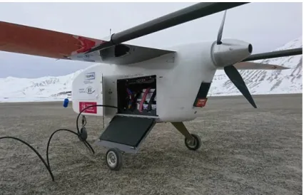
To carry out consecutive measurement operations over multiple hours, the aircraft was equipped with a side opening cargo door and sliding mechanism for a quick battery exchange and for copying the full data set, to minimize the turnaround time to around 20 min despite the insulation (Figure3).
Figure 3.ALADINA during turnaround and saving data via downlink. The battery is stored in the back of the payload bay and can be removed easily by opening the side door. The full compartment was insulated. Photo: Alexander Peuker, TU Braunschweig.
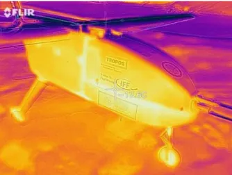
The development of the internal temperature and the corresponding air temperature was monitored during the flights. With the applied heating power and improved insulation, it was possible to maintain an increased internal temperature approximately 10 to 20◦C above the ambient air temperature during the flight. However, initially, the temperature decreased during flight, which is mainly caused by the increased heat transmission caused by cold air circulation of the airframe, the insufficient insulation and thermal bridges at the intersections of the compartments, as can be seen in the infrared image (Figure4). The insulation was improved significantly by sealing the intersections of the different parts of the fuselage. At the beginning of the campaign, during the flight on 24 April 2018, the deviation of the CPC temperatures of saturator and condensor were up to 1.5 K below the nominal value. After the additional insulation, the deviations were less than 0.5 K during the flight.
Monitoring of the internal temperatures was possible via data log and telemetry downlink.
Figure 4.Thermal infrared image of ALADINA. The thermal bridges are visible at the intersections of different compartments and were responsible for losses of heat during the flight.
Altogether, during the field campaign in Ny-Ålesund, ALADINA was proven to be a very flexible and reliable tool in the complex terrain. One of the most significant advantages is the removable payload bay with the scientific instrumentation. This makes maintenance and calibration very easy.
3.4. Impact of Rotor Blades on Quadrocopter Measurements and Data Processing (ALICE) 3.4.1. Observations
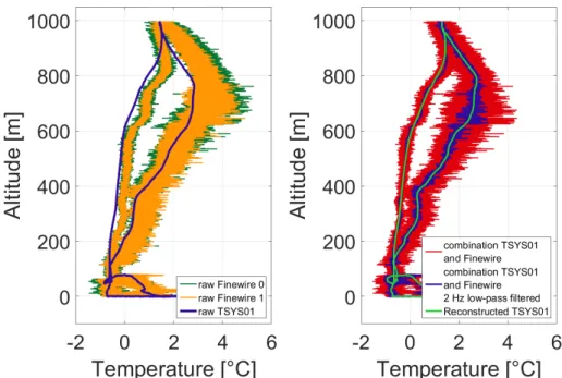
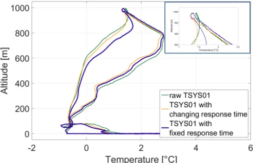
Profiles of the raw data of the two fine-wire temperature sensors revealed strong fluctuations (Figure5). The fluctuations were higher during descent than during ascent. For the slow sensors, the response time has to be taken into account. To retrieve the correct temperature values, the following correction processes were applied, as summarized in Figure6. The correction of the measurement signal is based on a first-order lag element (PT1) with an additional correction of the housing’s influence. All temperature and humidity sensors were installed in a housing for protection from radiation (Figure2). However, the heat capacity of the housing itself influences the temperature signal.
Due to this, an additional correction was performed, taking the dynamic pressure into account that was measured in the housing. The influence of the housing’s capacity was determined with the fast fine-wire sensors and then subtracted from the TSYS01 signal (see Figure6, process shaded in red).
Figure 5. (Left): ALICE raw profiles of temperature obtained with different sensors on 1 October 2017: Two fine-wire sensors (green and orange) with fast response time, and the digital TSYS01 sensor (blue) with slow response time. Descent is the line with higher fluctuations. (Right): ALICE profiles of processed temperature data: Combination of the high-pass filtered signal of the fast fine-wire “Finewire 0” and the low-pass filtered signal of the slow TSYS01 sensor (red), same combined signal but smoothed with a 2 Hz low-pass filter (blue), and reconstructed signal of the slow sensor TSYS01 after applying the methods shown in Figure6(green). “Finewire 1” is not used for the processing here, but shows that the features are reproducible.
Figure 6.Reconstruction of the temperature signal for ALICE raw measurements. During the first step of the reconstruction, shaded in red, the influence of the housing is corrected via use of the fast fine-wire sensor. During the second step, indicated in blue, complementary low and high-pass filtering with a frequency of 1/30 Hz is applied. During the final step, the signal is low-pass filtered.
Subsequently, the actual reconstruction was performed with the low-pass filtered signal (<1/30 Hz) of the TSYS01 based on a PT1-element. A Butterworth filter of first order was applied (resulting in the green line in Figure5, right panel). Finally the high-pass filtered signal (>1/30 Hz) of the fine-wire sensor was added to the reconstructed signal (process shaded in blue in Figure6, resulting in the red line in Figure5, right panel). For better visualization, based on the spectrum of the fine-wire signal, the combined signal was low-pass filtered at 2 Hz (process shaded in green in Figure6). The result shows the combination of the low-pass long-term stable TSYS01 sensor with the high-pass filtered fast fine-wire temperature sensor (blue line in Figure5, right panel).
The current time constants were determined as a function of the velocity of the quadrocopter.
According to the data sheet, the response time of the TSYS01 is 4 s, determined for a temperature change from 25◦C to 75◦C and a flow velocity of 60 m s−1. The flow speed v impacting the sensor was estimated by measuring the dynamic pressureqin the housing of the sensors:
q=1/2·ρ·v2 (1)
Here,ρis the air density determined from the static pressure.
The response time was not corrected by a fixed value, but was tied to the vertical velocity.
Applying a variable response time gives the opportunity to handle the dynamic behavior of the measurement system. While ALADINA has a nearly constant air flow around the sensors, ALICE’s sensors have changing flow directions and flow rates. The changing conditions are based on the different layouts of the systems (see Figure 7). A flight usually includes hovering, ascent and decent phases with different airflow rates through the sensor housing. The assumption was that different airflow rates cause different velocities in heat transfer (e.g., during ascent the air flow of the quadrocopter is added to the air flow induced by the propellers). Doing so, the first derivative of the altitude was used, normalized, and multiplied to the response time. A further constraint was the assumption of small changes in the meteorological parameter within small spatial distances and short temporal delays (e.g., in the turning point). This method results in a response time of around 5 s during ascent with a vertical speed of 6.5 m s−1(see Figure7), and around 10 s for hover.
Figure 7. Reconstruction of the temperature signal of the raw slow TSYS01 sensor measurements (green) by applying constant (purple) and variable (yellow) response times, depending on the flow velocity. The line with lower temperatures corresponds to the ascent.
3.4.2. Simulations
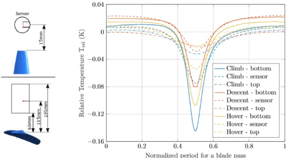
The fast responding fine-wire sensors of the quadrocopter show high temperature fluctuations depending on the flight state (Figure5). The possibility of an electronic or vibratory source of noise has been discarded. Based on the approach presented in [21], these perturbations can be due to frictional or compressible heating, turbulent fluctuations, radiated heat from the motor, or a general decoupled sensor from the environment in stagnating flow. Numerical simulations for climb, hover, and descent flight state were performed in order to assess propeller blade induced effects.
Unsteady Reynolds-Averaged Navier Stokes (URANS) simulations with the Shear Stress Transport (SST) turbulence model were performed using the software ANSYS CFX, taking one of the propellers
of the multicopter as the main geometry, being enclosed in a fluid domain. The simulations were transient in nature, using moving meshes in order to take into account the rotation of the propeller.
The angular speed of the propeller and the incoming flow velocity were set according to the condition being simulated: 6.5 m s−1and 3912 RPM (rounds per minute) for climb, 0 m s−1and 3120 RMP for hover and−2 m s−1and 2880 RPM for descent. The flow was considered compressible, obeying the ideal gas law, having an ambient temperature of 0◦C and ambient pressure of 1 atm at the boundaries.
Figure8depicts the distribution of the relative temperature (Trel =T−Tamb) in the surroundings of the blade during climb flight. As can be seen, the temperature is affected due to compressibility and viscous work effects induced by the blade. The color scale is capped between the values ofTrelof
−0.25 K and 0.25 K, although at the wing tipTrelcan reach values of 9.1 K in climb flight and 4.9 K in descent flight.
Figure 8. Top view showing the contours of relative temperature during climb flight at 6.5 m s−1. The relative temperature varies between−0.25 and 0.25 K, although lower or higher values can be reached near the surface of the propeller.
Figure9presents the temperature simulations for points where the sensors and the sensor shield inlet (top) and outlet (bottom) are located in order to show the perturbations that the propeller induces in the surrounding temperature field. It can be seen that the temperature of the fast fine-wire sensor is significantly impacted by the blade rotation. Compressibility leads to a reduced temperature when the blade passes under the sensor and, afterwards, dissipated heat from the flow increases the temperature until the next blade passes. These effects become stronger the smaller the distance to the blade. In the descent flight state, generated vortices carry more heat from the downwash of the propeller back to the top, where the sensor is located. Additional effects on the temperature by the sensor shield and heat dissipated by the motor may be present and are subject of further numerical investigations.
Figure10shows the simulated air temperature spectra at the location of the fine-wire sensor for the different flight states. Due to the two rotor blades per propeller, the blade rotational speed of 48 Hz for descent, 52.8 Hz for hover and 65.2 Hz for climb result in a first harmonics frequency of 96 Hz, 105.6 Hz, and 130.4 Hz, which are indicated in Figure10by vertical lines. Additionally, strong unsteady flow behavior due to flow re-circulation induces stronger lower frequency fluctuations in descent flight when compared to the hover and climb flight states. For the measurement frequency of 100 Hz, strong temperature fluctuations during descent can be resolved. However, the temperature fluctuations induced during climb at frequencies above 100 Hz cannot be resolved.
Figure 9.(Upper left): Top view of geometry of fine-wire temperature sensor and housing, and its relative positioning to the rotor blade (blue) at closest approach. (Lower left): Side view of the propeller blade (blue), the housing and the location of the fine-wire sensor within the housing. (Right): Relative temperature changes during a blade pass for different states (hover, climb, descent) and different locations of the sensor with respect to the propeller blades.
Figure 10.Simulations of temperature spectra (amplitude of temperature fluctuations over frequency) at the sensor location for climb (blue), descent (orange) and hover (yellow). The vertical lines represent the first harmonics of the blade rotational speed in the respective colors.
Simulations and measurements do not contradict each other. However, the simulation of the air temperature does not yet include the heat transfer between air and the fine-wire elements, and the effects of analogue-digital downsampling. The impact of the rotor blades on temperature measurements is in the same order of magnitude as described in [36].
3.5. Icing (M2AV)
A main challenge of operating UAS in polar environments is the frequent occurrence of icing conditions. Ice builds up rapidly, changes the aerodynamics, and adds weight while the effectiveness of the control surfaces is degrading very fast. Icing of the pitot tube leads to wrong indications of the true air speed [37].
With the M2AV, icing occurred during a flight at low altitudes on 2 August 2013, although icing conditions were considered as not likely based on the forecast and the visual impression before take-off.
However, after landing, ice was obvious at the wings (Figure11a) and the meteorological sensors (Figure11b), and the mass of the whole system had increased by 1.5 kg.
Figure 11.Ice on the wing (a) and meteorological sensors (b) of the M2AV after landing on 2 August 2013. Photo: Andreas Scholtz, TU Braunschweig.
The impact of icing on the aerodynamics can further be seen in the flight data shown in Figure12.
Within 10 min, there is a gradual decrease of the true air speed and an increase of the angle of attack to compensate the loss of lift. Due to the gained weight, the true air speed decreased to almost 17.5 m s−1 between 02:20 and 02:21 UTC, so that stall was likely.
Figure 12. Time series of the angle of attack (top) and the true air speed (bottom) from the M2AV during icing on 2 August 2013.
4. Examples of Specific Scientific Applications of UAS in Polar Areas
In the following, examples of measurements with the mentioned UAS in the polar areas are shown. They intend to illustrate the broad range of research questions that can be addressed with these systems.
4.1. Temperature and Wind Fluctuations Observed above Open Water Sections (M2AV)
During the winter cruise with the RVPolarsternin 2013, the M2AV was on board and first results are presented in Jonassen et al. [16]. The aim was to quantify the impact of leads on the atmospheric boundary layer.
UAS measurements of meteorological parameters above the Terra Nova Bay polynya without high temporal resolution for fluxes have been performed [38]. With the M2AV, turbulent fluxes of momentum and sensible heat were analyzed for one particular ice station, where RVPolarsternwas located from 29 July to 2 August 2013. The sea ice drift was around 0.14 km h−1, calculated from the GPS coordinates of the vessel that are publicly available [39]. The sea ice concentration was 90% and the size of individual floes varied between 100 to 500 m, taken from the sea ice observations [40] (see Figure13for a picture of the ice conditions as seen from the ship). In the direct surrounding of the Polarstern, a narrow opening was present like a small crack that was partly frozen. At a distance of around 4 km, SE of the RV, there was an open lead. The M2AV performed two flights perpendicular to the open water sections, starting near the ship from NW to SE and back from SE–NW. Flight legs were performed horizontally at different heights of 15, 25, 50, 75, and 150 m ASL (not all shown here) with a distance of around 4–4.5 km from the research vessel. During the flight, the mean wind direction was from South with a mean wind speed of 10 m s−1, measured at the RV [39], so that the observations were performed almost across the plume resulting from the warm water sectors above the lead.
Figure 13.Ice conditions during the ice station ofPolarsternon 2 August 2013. The flight path of the M2AV is indicated as black dashed line. The locations of open water that were investigated during perpendicular flights are shown in red. Photo: Stefan Hendricks, AWI.
Figure14shows the fluctuations of the three wind vector components calculated along the flight track at three different heights (75, 50 and 25 m) perpendicular to the open lead. The blue shaded boxes point out the approximate position of the small opening between 0.5 and 1.1 km distance and the lead in the distance of around 2.4 and 4.5 km. The time series of wind speed show only a weak dependence on the surface variability. The fluctuations of the three wind vector components are slightly enhanced above the lead in the second sector shaded in blue, but not above the small opening near the ship, at least for the altitudes that were sampled. The onset of fluctuations of the wind vector components starts at a later point, not directly above the beginning of the open water. Here, it has to be considered
that position and width of the open water is only based on personal observations. Neither a camera system nor a surface temperature sensor were installed on board the UAS that might verify the actual position of the lead. Furthermore, a clear evidence of homogeneous ice-free conditions of the lead is not assured. However, the data are nonetheless significant in its unique observations in the Weddell Sea during winter time.
0 0.5 1 1.5 2 2.5 3 3.5 4 4.5
-2 -1 0 1 2
Wind speed fluctuation(m s-1)
u' v' w' 75 m
0 0.5 1 1.5 2 2.5 3 3.5 4 4.5
-2 -1 0 1 2
50 m
Wind speed fluctuation(m s-1)
0 0.5 1 1.5 2 2.5 3 3.5 4 4.5
-2 -1 0 1 2
Distance - Polarstern (km) Wind speed fluctuation(m s-1)
25 m
Figure 14.Time series of wind speed fluctuations during the M2AV flights at 75, 50 and 25 m altitude (from (top) to (bottom)). The three components of the wind speed vector are defined positive as eastwards (black), northwards (red) and upwards pointing (blue). The parts of the flight track above open water are indicated by light blue boxes.
Above the large lead of more than 2 km width at around 2.4 km distance, temperature fluctuations are enhanced (Figure15). This is not the case for the small crack of around 600 m length at the distance of 500 m. The onset of enhanced fluctuations are in agreement with the open water sectors for the altitudes 25 and 50 m. For the highest altitude of 75 m, the onset of enhanced turbulent fluctuations of temperature appears later above the lead, as observed for the fluctuations of the wind vector components. This results from the South wind direction along the flight track (transporting air masses towards the lead). It is in agreement with an internal mixed layer building up in the stably stratified boundary layer [41].
Concerning the surface-based temperature inversion, the flight altitudes were chosen in mostly stable conditions in the lowermost 200 m. A strong inversion layer was observed between 80 and 130 m.
This can be taken from the radiosonde that was launched at 11:03 UTC from the RV [42] (Figure16a, grey circle). The horizontal M2AV flights were performed 2 h later between 13:04 and 13:48 UTC.
Turbulent fluxes were computed via the covariance method of measured vertical wind speed and temperature. Averaging was applied for 1 km steps along the leg crossing the plume perpendicular to the lead. Thus, the last quarter of turbulent kinetic energy (TKE) and sensible heat flux correspond to the section above open water. Calculated TKE and sensible heat flux are shown at the altitudes of 25, 50, and 75 m in Figure16b,c, marked with grey diamonds. The mixed layer, where the impact of the open water sections to the atmosphere is visible, can be seen in the small sensible heat flux of almost 30 W m2at the lower altitude of 25 m (Figure16c).
For comparison, an idealized quasi-2D model simulation of the turbulent flow over the observed lead was performed using the microscale but non-eddy-resolving model METRAS [43,44]. This model had already been applied for idealized simulations of lead scenarios (see e.g., [5]). Due to grid sizes of 100 m in horizontal and 20 m in vertical direction, the convective plume developing over the lead is resolved, but turbulent eddies still have to be parameterized. For simplicity, a local mixing-length closure was applied [45]. Thus, non-local transport is not considered, but basic features
of the flow structure can be reproduced (see [5]). The observed lead was idealized by assuming a constant width of 2.1 km, a constant surface temperature derived from the measurements, and by considering the radiosonde data for the initial inflow conditions of the simulation (see Figure16a for the potential temperature. The lead-averaged simulated profiles of TKE and sensible heat flux are shown in Figure16b,c (black lines) in comparison to the measurements of the M2AV. The simulated TKE is diagnosed from the modelled eddy diffusivity for momentum (Km) and stability corrected mixing length (see [44], their Equation (3.55). Here, the simulated lead-averaged values are, in general, smaller than the observed values, which could be explained by the potential underestimation ofKm
using a local closure in strong convective conditions [46].
-0.4 -0.2 0 0.2 0.4
Temperature fluctuation (K)
75 m
-0.4 -0.2 0 0.2 0.4
Temperature fluctuation (K)
50 m
0 0.5 1 1.5 2 2.5 3 3.5 4 4.5
-0.4 -0.2 0 0.2 0.4
Distance - Polarstern (km) Temperature fluctuation (K)
25 m
Figure 15.Time series of temperature fluctuations during the M2AV flights at 75, 50 and 25 m altitude (from (top) to (bottom)). The parts of the flight track above open water are indicated by blue boxes.
The simulated lead-averaged values of the sensible heat flux are approximately 29 Wm−2at a height of 25 m, 4 Wm−2at 50 m, and−2 Wm−2at 75 m. These values are marginally higher than the measured values. One possible explanation for this small deviation is that the simulation is still an idealized scenario although the model’s initial values are determined based on the measurements.
In addition, flights with the M2AV were performed perpendicular and not parallel to the lead so that the measured fluxes might have been underestimated [41]. Furthermore, in contrast to the idealized simulation, the lead edges observed on 2 August 2013 were not perfectly linearly shaped and, thus, the estimated lead width of 2.1 km represents a rough approximation only.
In addition, Figure17shows simulation results of wind speed and air temperature with respect to the distance toPolarstern. Note that the small crack between 0.5 and 1.1 km distance was not considered in the simulation. The influence of the lead on the wind field and the temperature distribution is also represented well and in agreement with the measurements. This study shows that such measurements may be helpful for the validation of models in many aspects.
From thermal satellite imagery from the Moderate Resolution Imaging Spectroradiometer (MODIS) with a resolution of 1 km at nadir, the potential open water area was 0.1 for the pixel includingPolarstern(Figure18), so the sea ice concentration was 90%. Cracks are visible in the area aroundPolarstern; however, the small leads investigated in the study cannot be resolved explicitly by MODIS imagery.
Figure 16.Three different observed and modelled quantities against altitude above ground level (AGL) for the area around the lead observed on 2 August 2013. (a) potential temperature measured with the radiosonde from RV at 11:03 UTC (grey circles, [42] and the corresponding inflow profile for the idealized simulation with the non-eddy resolving model METRAS (black lines). (b,c) observed values (grey diamonds) and lead-averaged simulation results (black lines) of the turbulent kinetic energy (TKE) and the sensible heat flux. The observed values were calculated from the M2AV flight legs at the three altitudes of 25, 50 and 75 m. The time of the flights was 13:04 to 13:48 UTC.
Figure 17.Wind speed in m s−1(top) and atmospheric temperature in◦C (bottom) at different height levels (25 m, 50 m, and 75 m) obtained from an idealized simulation of the lead observed on 2 August 2013 with the non-eddy resolving model METRAS. The results are shown with respect to the distance to RVPolarsternin km (see Figure13), as in Figures14and15. The flow is from right to left and the position of the lead is denoted by the blue rectangle between 2.4 km and 4.5 km distance. The observed small crack between 0.5 and 1.1 km distance (see Figure13) is not considered in the simulation.
The numerical simulations of [47] confirm that it is important to sample the atmosphere at very low altitude (<100 m) for spatially inhomogeneous sea surface conditions to derive information on the radiation budget. The same is confirmed by the simulations shown above.
Figure 18. Ice surface temperature (a) as seen from the MODIS sensor and derived potential open water (b). The scene was acquired by the satellite Terra at 04:55 UTC on 31 July 2013. The green crosses in the middle indicate the position ofPolarstern. Grey areas are masked due to land and cloud coverage.
4.2. Meteorological Profiling from Research Vessel (ALICE)
During the RV Polarstern expedition in autumn 2017, the development of the atmospheric boundary layer was investigated with ALICE vertical profile flights up to 1000 m altitude. The data are available at [17].
The short-term variability of the atmospheric boundary layer can be investigated by consecutive profiles. On 30 September and 1 October 2017, the general synoptic situation was characterized by southerly wind directions and low wind speed near the surface. An example of temperature profiles obtained on 30 September and 1 October 2017 is provided in Figure19. Significant temperature changes of up to 2 K are visible at the same altitude within short time intervals of few minutes (e.g., see temperature difference at 700 m altitude for the profiles on 1 October 2017 at 17:57 and 18:05 UTC).
Close to the surface in the lowermost 70 m, the temperature during the ascents was higher for all UAS flights than during descent. The measured UAS temperature is probably influenced byPolarsternas a source of heat. Multiple temperature inversions are present for almost all profiles, radiosonde and UAS based. They are typical for non-homogeneous sea ice conditions and have been observed in the Arctic [48] and Antarctic [16]. The fine structure is of importance for stability, enabling or dampening vertical transport.
Figure 19.Profiles obtained from three flights with quadrocopter ALICE on 30 September and 1 October 2017 and four radio sondes. The times are provided in UTC. The ascents are provided in brighter colors (cyan, bright green, orange), and the descents in darker colors (blue, dark green, red).
4.3. Instrumentation to Detect Ultrafine Aerosol Particles in the Arctic (ALADINA)
Ultrafine aerosol particles with diameters (DP)<20 nm have been observed at ground based stations and during ship borne campaigns in the Arctic. These particles are typically freshly formed due to nucleation and subsequent growth [49]. Airborne observations of new particle formation in Arctic areas are still rare. The events are typically characterized by low formation and growth rates [50].
To understand the process and potential sources, vertical measurements of these small particles are needed. Aerosol instruments on UAS have been used for different studies, e.g., [51,52].
The UAS ALADINA was equipped with instrumentation to measure ultrafine aerosol particles in different size ranges in the Arctic. This was realized by a combination of two modified CPCs implemented on the UAS ALADINA. CPCs typically contain a heated saturator unit, saturated with a working fluid. Afterwards, the saturated sample flow is led into a cooled condensor unit, where the fluid is condensing on the particle surface and ensures that the particles grow to a detectable size.
The temperature difference between saturator and condensor defines the lower detection range of a CPC. Using this relation, the detection limit of a CPC can be changed within certain limits: Higher temperature differences cause lower detection limits [53].
The two ALADINA CPCs were modified and characterized in the laboratory of the Leibniz Institute for Tropospheric Research (TROPOS). The temperature difference of CPC1 was set to 18 K and that of CPC2 to 7 K. The differences between the actual and nominal temperatures of the condensors and saturators for both CPCs was monitored during the flights, and was continuously within a±0.5 K-band around the set point temperature, in particular after the additional insulation. The resulting counting efficiency and fitted curve for both instruments are shown in Figure20. The lower detection limit of a CPC is typically given as the diameter where the counting efficiency of the instrument is 50%. This diameter is calledDP50and can be obtained from measurements in the laboratory using a defined aerosol source at different particle diameters in comparison to a reference [54]. Due to the low variation in saturator and condensor temperatures, thisDP50is very stable; the variation is assumed to be less than 1 nm. The resultingDP50are 3.3 and 12.2 nm. The difference between both number concentrations is the number concentration between 3.3 and 12.2 nm and thus a measure for ultrafine particles.
Figure 20.Counting efficiency of the two modified CPCs operated on-board ALADINA. Dots and stars show the measured values at selected diameters, while the line shows a fit according to the equation and coefficients in the textbox above. TheDP50of CPC 1 is 3.3 nm that of CPC 2 is 12.2 nm.
Implemented into ALADINA, the CPCs provide a tool to measure the vertical distribution of aerosol particle number concentrations in three different size ranges:>3.3 nm,>12.2 nm, and 3.3 nm
<DP<12.2 nm with a time resolution of approximately 1 s.
4.4. Vertical Distribution of Aerosol in Svalbard (ALADINA)
ALADINA was used as a link between different aerosol observatories in Svalbard (Norway).
Research flights were performed in spring 2018 at the airfield in Ny-Ålesund and first results are presented in [18]. The research village of Ny-Ålesund is located at Kongsfjord and surrounded by mountains up to 700 m ASL and glaciers. The flow is highly influenced by complex terrain [55,56], so that aerosol properties in the valley and on top of the mountain may be very different [57]. Vertical profiles of ultrafine aerosol particle may help to locate the regions where new particle formation and growth take place.
Figure21shows vertical profiles measured during three different flights between 9:15 and 13:15 on 15 May 2018 up to a maximum height of 850 m AGL with ALADINA. The meteorological parameters potential temperatureθand water vapor mixing ratioqare shown on the left-hand side and illustrate the vertical stratification for each profile. During the observed period, the vertical structure has changed significantly. In general, the lowest 800 m AGL are characterized by a stably stratified layer, but the gradient of the potential temperature varies vertically and also temporally. The profile of water vapor mixing ratio changes between the flights, in the first oneqdecreases up to a height of 600 m AGL and remains constant above. This gradient disappears during the following flights and during the profile flown at 13:04, whereqis nearly constant with height. The plots on the right-hand side show the corresponding profiles of aerosol particle number concentration (N): CPC1 measures aerosol particles withDP>3 nm and CPC2 withDP>12 nm. The difference between both CPCs is not significant, thus we can conclude that the number concentration of particles between 3 and 12 nm is negligible. In addition, these profiles show that the vertical structure is changing. While during the first flight at 09:15 UTCNdecreases nearly linearly with height, strong gradients are visible in the following flights. In the first flight, one sharp gradient appears at 350 m AGL (above ground level) corresponding to an inversion visible by the increase of potential temperatureθ. At 11:52 and 13:04 UTC,Nis nearly constant above 400 m AGL and increases below. Here, the strong inversion obviously suppresses the vertical exchange of aerosol particles emitted on the ground. The number concentration of larger particles (>390 nm) measured by OPC shows a different picture with nearly constant values over height. This means that the maximum inNmeasured by the two CPCs is caused by particles with diameters<390 nm.
The plots illustrate the vertical variability of aerosol particle number concentration for this case study. During different meteorological conditions, the profiles may look completely different.
From these results, one can conclude that measurements at fixed heights, e.g., Gruvebadet (40 m AGL) and Zeppelin Mountain (475 m AGL) cannot describe the vertical structure of aerosol distribution and vertical measurements are essential in order to study transport and formation processes of aerosol particles.
Figure 21. Three vertical profiles of potential temperature, water vapor mixing ratio, and aerosol particle number concentration, measured during three different flights with ALADINA on 15 May 2018.
5. Conclusions
Three different UAS and examples of their missions showed the broad range of applications and the capabilities of such systems in the polar regions. Besides exemplary scientific results, the focus was on adaptations to enable flexible and reliable applications in cold environments with temperatures below –20◦C. All three examples demonstrate the importance of flexible small-scale high-resolution measurements, which are only possible with UAS: The M2AV flights allow investigations close to the surface. With a very shallow polar atmospheric boundary layer, flight levels below 100 m are required. For future measurements, the sampling strategy should focus on retrieving the atmospheric stratification first, and then choose the altitude of the flight legs accordingly. Additionally, the implementation of a fast and light-weight humidity sensor on the fixed-wing systems would allow for retrieving latent heat fluxes. Such systems have been operated by e.g., [29,35,58].
For measurement flights directly from the ship, the local influence of artificial heat sources on the measurements has to be taken into account. Ideally, quadrocopter measurements should be first directed into an area not affected by the ship’s plume, and then begin the profiling from directly above the surface up to the required altitude. More detailed simulations are required to reproduce the effect of flow around a multicopter and the impact on sensors. The necessary steps for further detailed system identification can be derived from this.
With the ALADINA measurements, it is possible to provide a link for understanding aerosol properties from observatories and relate them to the complex orography. In such environments, ground-based measurements are not sufficient to study transport and formation processes and continuous profiling is needed to improve the understanding of aerosol processes. In a future study, the case will be investigated with additionally taking into account atmospheric parameters like stability, wind field, and turbulence in combination with numerical simulations.
Author Contributions:B.A., A.S., F.P., T.K., K.B., L.B., R.K., A.P., and B.W. participated in the field campaign and collected the data. A.S., F.P., K.B., L.B., M.H., R.K., T.K., S.N., A.P., and A.S. prepared the UAS and data acquisition systems for the polar missions. F.P., B.A., K.B., B.W., and A.L. processed and analyzed the data. D.S.Z., D.G., and S.B. developed the model for studying the impact of the rotor blades on the measurement signals. C.L., E.D., and A.L. planned the flight strategies. J.M. and C.L. performed the simulations of fluxes. F.R. prepared the sea ice charts of the Weddell Sea. A.L., B.A., and F.P. wrote the manuscript, and A.L., B.A., K.B., L.B., J.S., J.M., L.L., M.A., E.D., R.K., T.K., C.L., S.N., A.P., T.R., F.R., A.S., D.S.Z., D.G., S.B., B.W., F.P. contributed to the text and figures. All authors have read and agreed to the published version of the manuscript.
Funding:The measurements of ALADINA in Svalbard were funded by the German Research Foundation under grant LA2907/5-3. The development of ALICE and the measurements in the Arctic were funded by the German Research Foundation DFG Priority Program “Antarctic Research with comparative investigations in Arctic ice areas” under grant LA2907/8-1. The participation to thePolarsterncruise in the Weddell Sea has been funded by the Alfred Wegener Institute. The atmospheric modelling part was supported by the German Research Foundation (grant LU 818/5-1).
Acknowledgments: The authors would like to thank Markus Hermann of TROPOS for his support with the aerosol sensors. The authors gratefully acknowledge AWIPEV and Kingsbay for assistance prior and especially during the field study at Ny-Ålesund, and the colleagues from the University of Tübingen, in particular Jens Bange, Andreas Platis and Martin Schön for the successful campaign.
Conflicts of Interest:The authors declare no conflict of interest. The funders had no role in the design of the study; in the collection, analyses, or interpretation of data; in the writing of the manuscript, or in the decision to publish the results.
References
1. Konrad, T.G.; Hill, M.L.; Rowland, J.R.; Meyer, J.H. A Small, Radio-Controlled Aircraft As A Platform For Meteorological Sensors.Johns Hopkins APL Tech. Dig.1970,10, 11–21.
2. Emeis, S.; Kalthoff, N.; Adler, B.; Pardyjak, E.; Paci, A.; Junkermann, W. High-Resolution Observations of Transport and Exchange Processes in Mountainous Terrain.Atmosphere2018,9, 457. [CrossRef]
3. Intrieri, J.M.; de Boer, G.; Shupe, M.D.; Spackman, J.R.; Wang, J.; Neiman, P.J.; Wick, G.A.; Hock, T.F.; Hood, R.E. Global Hawk dropsonde observations of the Arctic atmosphere obtained during the Winter Storms and Pacific Atmospheric Rivers (WISPAR) field campaign.Atmos. Meas. Tech.2014,7, 3917–3926. [CrossRef]
4. Andreas, E.L.; Cash, B.A. Convective heat transfer over wintertime leads and polynyas.J. Geophys. Res.1999, 104, 25721–25734. [CrossRef]
5. Lüpkes, C.; Gryanik, V.M.; Witha, B.; Gryschka, M.; Raasch, S.; Gollnik, T. Modeling convection over arctic leads with LES and a non-eddy-resolving microscale model.J. Geophys. Res.2008,113, 1–17. [CrossRef]
6. Lüpkes, C.; Vihma, T.; Birnbaum, G.; Wacker, U. Influence of leads in sea ice on the temperature of the atmospheric boundary layer during polar night.Geophys. Res. Lett.2008,35, L03805. [CrossRef]
7. Soddell, J.R.; McGuffie, K.; Holland, G.J. An in-flight airframe icing nowcast for use with the Aerosonde. In Proceedings of the 10th Conference on Aviation, Range, and Aerospace Meteorology, Portland, ON, USA, 13–16 May 2002; Conference Paper P4.5, 4p. Available online: https://ams.confex.com/ams/13ac10av/
techprogram/paper_38619.htm(accessed on 10 October 2019).
8. Bates, T.S.; Quinn, P.K.; Johnson, J.E.; Corless, A.; Brechtel, F.J.; Stalin, S.E.; Meinig, C.; Burkhart, J.F.
Measurements of atmospheric aerosol vertical distributions above Svalbard, Norway, using unmanned aerial systems (UAS).Atmos. Meas. Tech.2013,6, 2115–2120. [CrossRef]
9. Curry, J.A.; Maslanik, J.; Holland, G.; Pinto, J. Applications of Aerosondes in the Arctic.Bull. Am. Meteor. Soc.
2004,85, 1855–1861. [CrossRef]
10. Telg, H.; Murphy, D.M.; Bates, T.S.; Johnson, J.E.; Quinn, P.K.; Giardi, F.; Gao, R.-S. A practical set of miniaturized instruments for vertical profiling of aerosol physical properties. Aerosol Sci. Technol. 2017, 51, 715–723. [CrossRef]
11. Fraser, R.H.; Olthof, I.; Lantz, T.C.; Schmitt, C. UAV photogrammetry for mapping vegetation in the low-Arctic.Arct. Sci.2016,2, 79–102. [CrossRef]
12. Riihimäki, H.; Luoto, M.; Heiskanen, J. Estimating fractional cover of tundra vegetation at multiple scales using unmanned aerial systems and optical satellite data.Remote Sens. Environ.2019,224, 119–132. [CrossRef]
13. Lehmenhecker, S.; Wulff, T. Flying Drone for AUV Under-Ice Missions.Sea Technol.2013,55, 61–64.
14. Bash, E.A.; Moorman, B.J. Surface melt and the importance of water flow—An analysis based on high-resolution unmanned aerial vehicle (UAV) data for an Arctic glacier. Cryosphere2020,14, 549–563.
[CrossRef]
15. Cimoli, E.; Marcer, M.; Vandecrux, B.; Bøggild, C.E.; Willims, G.; Simonsen, S.B. Application of Low-Cost UASs and Digital Photogrammetry for High-Resolution Snow Depth Mapping in the Arctic.Remote Sens.
2017,9, 1144. [CrossRef]
16. Jonassen, M.O.; Tisler, P.; Altstädter, B.; Scholtz, A.; Vihma, T.; Lampert, A.; König-Langlo, G.; Lüpkes, C.
Application of remotely piloted aircraft systems in observing the atmospheric boundary layer over Antarctic sea ice in winter.Polar Res.2015,34, 25651. [CrossRef]