A Tutorial on
Linear and Differential Cryptanalysis
by
Howard M. Heys
Electrical and Computer Engineering Faculty of Engineering and Applied Science
Memorial University of Newfoundland St. John’s, NF, Canada A1B 3X5
email: howard@engr.mun.ca
Abstract: In this paper, we present a detailed tutorial on linear cryptanalysis and differential cryptanalysis, the two most significant attacks applicable to symmetric-key block ciphers. The intent of the paper is to present a lucid explanation of the attacks, detailing the practical application of the attacks to a cipher in a simple, conceptually revealing manner for the novice cryptanalyst. The tutorial is based on the analysis of a simple, yet realistically structured, basic Substitution-Permutation Network cipher.
Understanding the attacks as they apply to this structure is useful, as the Rijndael cipher, recently selected for the Advanced Encryption Standard (AES), has been derived from the basic SPN architecture. As well, experimental data from the attacks is presented as confirmation of the applicability of the concepts as outlined.
1. Introduction
In this paper, we present a tutorial on two powerful cryptanalysis techniques applied to symmetric-key block ciphers: linear cryptanalysis [1] and differential cryptanalysis [2].
Linear cryptanalysis was introduced by Matsui at EUROCRYPT ’93 as a theoretical attack on the Data Encryption Standard (DES) [3] and later successfully used in the practical cryptanalysis of DES [4]; differential cryptanalysis was first presented by Biham and Shamir at CRYPTO ’90 to attack DES and eventually the details of the attack were packaged as a book [5]. Although the early target of both attacks was DES, the wide applicability of both attacks to numerous other block ciphers has solidified the pre- eminence of both cryptanalysis techniques in the consideration of the security of all block ciphers. For example, many of the candidates submitted for the recent Advanced Encryption Standard process undertaken by the National Institute of Standards and Technology [6] were designed using techniques specifically targeted at thwarting linear and differential cryptanalysis. This is evident, for example, in the Rijndael cipher [7], the encryption algorithm selected to be the new standard. The concepts discussed in this paper could be used to form an initial understanding required to comprehend the design principles and security analysis of the Rijndael cipher, as well as many other ciphers proposed in recent years.
The paper is structured as a tutorial and, as such, is intended to not be rigorously mathematical. It introduces the basic concepts of linear and differential cryptanalysis but is by no means a definitive source for understanding all the many refinements and improvements of the attacks over the years. The basic purpose of the paper is to use a simple (yet somewhat realistic) cipher structure to study the most basic concepts of the two attacks. Other more formal discussions exist on the topic. For example, overviews of the attacks as applied to Substitution-Permutation Networks (the cipher structured to be considered in this paper) are presented in [8] and [9]. For a general introduction to block ciphers and their analysis, see [10].
The need for a tutorial on the attacks arises from the very difficult nature of both attacks and the lack of simplified, yet detailed, reference material describing the attacks.
Conventional cryptographic references and texts [11][12][13][14] generally present material on block ciphers in a very descriptive manner, with little detail illustrating the concepts of the attacks. Consequently, most published material detailing the attacks has a research focus and gives little intuition and explanation for the non-expert. When the basic concepts of the attack are described in the literature (as in Matsui’s and Biham and Shamir’s original papers), they are typically presented in reference to DES which is, in nature, somewhat convoluted in a manner which interferes with the understanding the cryptanalytic concepts.
2. A Basic Substitution-Permutation Network Cipher
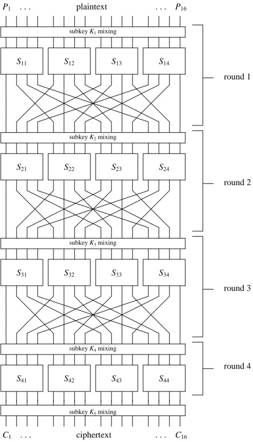
The cipher that we shall use to present the concepts is a basic Substitution-Permutation Network (SPN). We will focus our discussion on a cipher, illustrated in Figure 1, that takes a 16-bit input block and processes the block by repeating the basic operations of a round four times. Each round consists of (1) substitution, (2) a transposition of the bits (i.e., permutation of the bit positions), and (3) key mixing. This basic structure was presented by Feistel back in 1973 [15] and these basic operations are similar to what is found in DES and many other modern ciphers, including Rijndael. So although, we are considering a somewhat simplified structure, an analysis of the attack of such a cipher presents valuable insight into the security of larger, more practical constructions.
2.1 Substitution
In our cipher, we break the 16-bit data block into four 4-bit sub-blocks. Each sub-block forms an input to a 4×4 S-box (a substitution with 4 input and 4 output bits), which can be easily implemented with a table lookup of sixteen 4-bit values, indexed by the integer represented by the 4 input bits. The most fundamental property of an S-box is that it is a nonlinear mapping, i.e., the output bits cannot be represented as a linear operation on the input bits.
For our cipher, we shall use the same nonlinear mapping for all S-boxes. (In DES all the S-boxes in a round are different, while all rounds use the same set of S-boxes.) The attacks of linear and differential cryptanalysis apply equally to whether there is one mapping or all S-boxes are different mappings. The mapping chosen for our cipher, given in Table 1, is chosen from the S-boxes of DES. (It is the first row of the first S-box.) In the table, the most significant bit of the hexadecimal notation represents the leftmost bit of the S-box in Figure 1.
input 0 1 2 3 4 5 6 7 8 9 A B C D E F
output E 4 D 1 2 F B 8 3 A 6 C 5 9 0 7
Table 1. S-box Representation (in hexadecimal)
2.2 Permutation
The permutation portion of a round is simply the tranposition of the bits or the permutation of the bit positions. The permutation of Figure 1 is given in Table 2 (where the numbers represent bit positions in the block, with 1 being the leftmost bit and 16 being the rightmost bit) and can be simply described as: the output i of S-box j is connected to input j of S-box i. Note that there would be no purpose for a permutation in the last round and, hence, our cipher does not have one.
input 1 2 3 4 5 6 7 8 9 10 11 12 13 14 15 16
output 1 5 9 13 2 6 10 14 3 7 11 15 4 8 12 16 Table 2. Permutation
subkey K4 mixing subkey K3 mixing subkey K1 mixing
subkey K2 mixing
subkey K5 mixing
plaintext
. . . C16 . . . P16
P1 . . .
S21 S22 S23 S24
S11 S12 S13 S14
S31 S32 S33 S34
S41 S42 S43 S44
round 1
round 2
round 3
round 4
Figure 1. Basic Substitution-Permutation Network (SPN) Cipher C1 . . . ciphertext
2.3 Key Mixing
To achieve the key mixing, we use a simple bit-wise exclusive-OR between the key bits associated with a round (referred to as a subkey) and the data block input to a round. As well, a subkey is applied following the last round, ensuring that the last layer of substitution cannot be easily ignored by a cryptanalyst that simply works backward through the last round’s substitution. Normally, in a cipher, the subkey for a round is derived from the cipher’s master key through a process known as the key schedule. In our cipher, we shall assume that all bits of the subkeys are independently generated and unrelated.
2.4 Decryption
In order to decrypt, data is essentially passed backwards through the network. Hence, decryption is also of the form of an SPN as illustrated in Figure 1. However, the mappings used in the S-boxes of the decryption network are the inverse of the mappings in the encryption network (i.e., input becomes output, output becomes input). This implies that in order for an SPN to allow for decryption, all S-boxes must be bijective, that is, a one-to-one mapping with the same number input and output bits. As well, in order for the network to properly decrypt, the subkeys are applied in reverse order and the bits of the subkeys must be moved around according to the permutation, if the SPN is to look similar to Figure 1. Note also that the lack of the permutation after the last round ensures that the decryption network can be the same structure as the encryption network.
(If there was a permutation after the last substitution layer in the encryption, the decryption would require a permutation before the first layer of substitution.)
3. Linear Cryptanalysis
In this section, we outline the approach to attacking a cipher using linear cryptanalysis based on the example cipher of our basic SPN.
3.1 Overview of Basic Attack
Linear cryptanalysis tries to take advantage of high probability occurrences of linear expressions involving plaintext bits, "ciphertext" bits (actually we shall use bits from the 2nd last round output), and subkey bits. It is a known plaintext attack: that is, it is premised on the attacker having information on a set of plaintexts and the corresponding ciphertexts. However, the attacker has no way to select which plaintexts (and corresponding ciphertexts) are available. In many applications and scenarios it is reasonable to assume that the attacker has knowledge of a random set of plaintexts and the corresponding ciphertexts.
The basic idea is to approximate the operation of a portion of the cipher with an expression that is linear where the linearity refers to a mod-2 bit-wise operation (i.e., exclusive-OR denoted by "⊕"). Such an expression is of the form:
0 ...
... 1 2
2
1 ⊕ i ⊕ ⊕ iu ⊕ j ⊕ j ⊕ ⊕ jv =
i X X Y Y Y
X (1)
where Xi represents the i-th bit of the input X = [X1, X2, ...] and Yj represents the j-th bit of the output Y = [Y1, Y2, ...]. This equation is representing the exclusive-OR "sum" of u input bits and v output bits.
The approach in linear cryptanalysis is to determine expressions of the form above which have a high or low probability of occurrence. (No obvious linearity such as above should hold for all input and output values or the cipher would be trivially weak.) If a cipher displays a tendency for equation (1) to hold with high probability or not hold with high probability, this is evidence of the cipher’s poor randomization abilities. Consider that if we randomly selected values for u + v bits and placed them into the equation above, the probability that the expression would hold would be exactly 1/2. It is the deviation or bias from the probability of 1/2 for an expression to hold that is exploited in linear cryptanalysis: the further away that a linear expression is from holding with a probability of 1/2, the better the cryptanalyst is able to apply linear cryptanalysis. In the remainder of the paper, we refer to the amount by which the probability of a linear expression holding deviates from 1/2 as the linear probability bias. Hence, if the expression above holds with probability pL for randomly chosen plaintexts and the corresponding ciphertexts, then the probability bias is pL – 1/2. The higher the magnitude of the probability bias, |pL – 1/2|, the better the applicability of linear cryptanalysis with fewer known plaintexts required in the attack.
There are several ways to mount the attack of linear cryptanalysis. In this paper, we shall focus on what Matsui calls Algorithm 2 [1]. We investigate the construction of a linear approximation involving plaintext bits as represented by X in (1) and the input to the last
round of the cipher (or equivalently the output of the 2nd last round of the cipher) as represented by Y in (1). The plaintext bits are random and consequently so are the input bits to the last round.
Equation (1) could be equivalently reformulated to have the right side being the sum of a number of subkey bits. However, in (1) as written with the right side of "0", the equation implicitly has subkey bits involved: these bits are fixed but unknown (as they are determined by the key under attack) and implicity absorbed into the "0" on the right side of equation (1) and the probability pL that the linear expression holds. If the sum of the involved subkey bits is "0", the bias of (1) will have the same sign (+ or −) as the bias of the expression involving the subkey sum and, if the sum of the involved subkey bits is
"1", the bias of (1) will have the opposite sign.
Note that pL = 1 implies that linear expression (1) is a perfect representation of the cipher behaviour and the cipher has a catastrophic weakness. If pL = 0, then (1) represents an affine relationship in the cipher, also an indication of a catastrophic weakness. For mod-2 addition systems, an affine function is simply the complement of a linear function. Both linear and affine approximations, indicated by pL > 1/2 and pL < 1/2, respectively, are equally susceptible to linear cryptanalysis and we shall generally use the term linear to refer to both linear and affine relationships.
The natural question to ask is: How do we construct expressions which are highly linear and, hence, can be exploited? This is done by considering the properties of the cipher’s only nonlinear component: the S-box. When the nonlinearity properties of the S-box are enumerated, it is possible to develop linear approximations between sets of input and output bits in the S-box. Consequently, it is possible to concatenate linear approximations of the S-boxes together so that intermediate bits (i.e., data bits from within the cipher) can be cancelled out and we are left with a linear expression which has a large bias and involves only plaintext and the last round input bits.
3.2 Piling-Up Principle
Before we consider constructing a linear expression for the example cipher of this paper, we need some basic tools. Consider two random binary variables, X1 and X2. We begin by noting the simple relationships: X1⊕X2 = 0 is a linear expression and is equivalent to X1 = X2; X1⊕X2 = 1 is an affine expression and is equivalent to X1 ≠ X2.
Now, assume that the probability distributions are given by
=
−
= =
= 1 , 1
0 ) ,
( Pr
1 1
1 p i
i i p
X and
=
−
= =
= 1 , 1.
0 ) ,
( Pr
2 2
2 p i
i i p
X
If the two random variables are independent, then
=
=
−
−
=
=
−
=
=
−
=
=
=
=
=
1 , 1 , ) 1 )(
1 (
0 , 1 , )
1 (
1 , 0 , ) 1 (
0 , 0 , )
, ( Pr
2 1
2 1
2 1
2 1
2 1
j i p p
j i p
p
j i p
p
j i p
p j
X i X
and it can be shown that
Pr(X1 ⊕ X2 = 0) = Pr(X1 = X2)
= Pr(X1 = 0, X2 = 0) + Pr(X1 = 1, X2 = 1)
= p1p2 + (1−p1)(1−p2).
Another perspective is to let p1 = 1/2+ε1 and p2 = 1/2+ε2, where ε1 and ε2 are the probability biases and −1/2 ≤ ε1,ε2 ≤ +1/2. Hence, it follows that
Pr(X1 ⊕ X2 = 0) = 1/2 + 2ε1ε2
and the bias ε1,2 of X1 ⊕ X2 = 0 is
ε1,2 = 2ε1ε2.
This can be extended to more than two random binary variables, X1 to Xn, with probabilities p1 = 1/2+ε1 to pn = 1/2+εn. The probability that X1 ⊕ ... ⊕ Xn = 0 holds can be determined by the Piling-Up Lemma which assumes that all n random binary variables are independent.
Piling-Up Lemma (Matsui [1])
For n independent, random binary variables, X1, X2, ...Xn, Pr(X1 ⊕ ... ⊕ Xn = 0) = 1/2 +
∏
=
− n i
i n
1
2 1 ε
or, equivalently,
ε1,2,..,n =
∏
=
− n i
i n
1
2 1 ε
where ε1,2,..,n represents the bias of X1 ⊕ ... ⊕ Xn = 0.
Note that if pi = 0 or 1 for all i, then Pr(X1 ⊕ ... ⊕ Xn = 0) = 0 or 1. If only one pi = 1/2, then Pr(X1 ⊕ ... ⊕ Xn = 0) = 1/2.
In developing the linear approximation of a cipher, the Xi values will actually represent linear approximations of the S-boxes. For example, consider four independent random
binary variables, X1, X2, X3 and X4. Let Pr(X1 ⊕ X2 = 0) = 1/2 + ε1,2 and Pr(X2 ⊕ X3 = 0) = 1/2 + ε2,3 and consider the sum X1 ⊕ X3 to be derived by adding X1 ⊕ X2 and X2 ⊕ X3
together. Hence,
Pr(X1 ⊕ X3 = 0) = Pr([X1 ⊕ X2] ⊕ [X2 ⊕ X3] = 0).
So we are combining linear expressions to form a new linear expression. Since we may consider random variables X1 ⊕ X2 and X2 ⊕ X3 to be independent, we can use the Piling- Up Lemma, to determine
Pr(X1 ⊕ X3 = 0) = 1/2 + 2ε1,2ε2,3
and, consequently,
ε1,3 = 2ε1,2ε2,3.
As we shall see, the expressions X1 ⊕ X2 = 0 and X2 ⊕ X3 = 0 are analogous to linear approximations of S-boxes and X1 ⊕ X3 = 0 is analogous to a cipher approximation where the intermediate bit X2 is eliminated. Of course, the real analysis will be more complex involving many S-box approximations.
3.3 Analyzing the Cipher Components
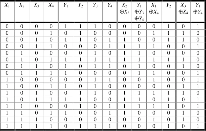
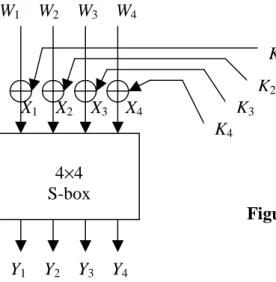
Before considering the attack in any more detail on the overall cipher, we first require knowledge of the linear vulnerabilities of an S-box. Consider the S-box representation of Figure 2 with input X = [X1 X2 X3 X4] and a corresponding output Y = [Y1 Y2 Y3 Y4]. All linear approximations can be examined to determine their usefulness by computing the probability bias for each. Hence, we are examining all expressions of the form of equation (1) where X and Y are the S-box input and outputs, respectively.
For example, for the S-box used in our cipher, consider the linear expression
4 0
3 1 3
2 ⊕X ⊕Y ⊕Y ⊕Y =
X or equivalently
4 3 1 3
2 X Y Y Y
X ⊕ = ⊕ ⊕ .
X1 X2 X3 X4
Y1 Y2 Y3 Y4 4×4
S-box Figure 2. S-box Mapping
Applying all 16 possible input values for X and examining the corresponding output values Y, it may be observed that for exactly 12 out the 16 cases, the expression above holds true. Hence, the probability bias is 12/16−1/2 = 1/4. This is presented in Table 3.
Similarly, for equation
2 4
1 X Y
X ⊕ =
it may be seen that the probability bias is 0 and for equation
4 1 4
3 X Y Y
X ⊕ = ⊕
the probability bias is 2/16−1/2 = −3/8. In the last case, the best approximation is an affine approximation as indicated by the minus sign. However, the success of the attack is based on magnitude of the bias and, as we shall see, affine approximations can be used equivalently to linear approximations.
X1 X2 X3 X4 Y1 Y2 Y3 Y4 X2
⊕X3
Y1
⊕Y3
⊕Y4
X1
⊕X4
Y2 X3
⊕X4
Y1
⊕Y4
0 0 0 0 1 1 1 0 0 0 0 1 0 1
0 0 0 1 0 1 0 0 0 0 1 1 1 0
0 0 1 0 1 1 0 1 1 0 0 1 1 0
0 0 1 1 0 0 0 1 1 1 1 0 0 1
0 1 0 0 0 0 1 0 1 1 0 0 0 0
0 1 0 1 1 1 1 1 1 1 1 1 1 0
0 1 1 0 1 0 1 1 0 1 0 0 1 0
0 1 1 1 1 0 0 0 0 1 1 0 0 1
1 0 0 0 0 0 1 1 0 0 1 0 0 1
1 0 0 1 1 0 1 0 0 0 0 0 1 1
1 0 1 0 0 1 1 0 1 1 1 1 1 0
1 0 1 1 1 1 0 0 1 1 0 1 0 1
1 1 0 0 0 1 0 1 1 1 1 1 0 1
1 1 0 1 1 0 0 1 1 0 0 0 1 0
1 1 1 0 0 0 0 0 0 0 1 0 1 0
1 1 1 1 0 1 1 1 0 0 0 1 0 1
Table 3. Sample Linear Approximations of S-box
Output Sum
0 1 2 3 4 5 6 7 8 9 A B C D E F
0 +8 0 0 0 0 0 0 0 0 0 0 0 0 0 0 0
1 0 0 −2 −2 0 0 −2 +6 +2 +2 0 0 +2 +2 0 0 2 0 0 −2 −2 0 0 −2 −2 0 0 +2 +2 0 0 −6 +2 3 0 0 0 0 0 0 0 0 +2 −6 −2 −2 +2 +2 −2 −2 4 0 +2 0 −2 −2 −4 −2 0 0 −2 0 +2 +2 −4 +2 0 5 0 −2 −2 0 −2 0 +4 +2 −2 0 −4 +2 0 −2 −2 0 6 0 +2 −2 +4 +2 0 0 +2 0 −2 +2 +4 −2 0 0 −2 7 0 −2 0 +2 +2 −4 +2 0 −2 0 +2 0 +4 +2 0 +2 8 0 0 0 0 0 0 0 0 −2 +2 +2 −2 +2 −2 −2 −6 9 0 0 −2 −2 0 0 −2 −2 −4 0 −2 +2 0 +4 +2 −2 A 0 +4 −2 +2 −4 0 +2 −2 +2 +2 0 0 +2 +2 0 0
B 0 +4 0 −4 +4 0 +4 0 0 0 0 0 0 0 0 0
C 0 −2 +4 −2 −2 0 +2 0 +2 0 +2 +4 0 +2 0 −2 D 0 +2 +2 0 −2 +4 0 +2 −4 −2 +2 0 +2 0 0 +2 E 0 +2 +2 0 −2 −4 0 +2 −2 0 0 −2 −4 +2 −2 0 I
n p u t S u m
F 0 −2 −4 −2 −2 0 +2 0 0 −2 +4 −2 −2 0 +2 0 Table 4. Linear Approximation Table
A complete enumeration of all linear approximations of the S-box in our cipher is given in the linear approximation table of Table 4. Each element in the table represents the number of matches between the linear equation represented in hexadecimal as "Input Sum" and the sum of the output bits represented in hexadecimal as "Output Sum" minus 8. Hence, dividing an element value by 16 gives the probability bias for the particular linear combination of input and output bits. The hexadecimal value representing a sum, when viewed as a binary value indicates the variables involved in the sum. For a linear combination of input variables represented as a1⋅X1⊕a2⋅X2⊕a3⋅X3⊕a4⋅X4 where ai ∈ {0,1}
and "⋅" represents binary AND, the hexadecimal value represents the binary value a1a2a3a4, where a1 is the most significant bit. Similarly, for a linear combination of output bits b1⋅Y1⊕ b2⋅Y2⊕ b3⋅Y3⊕ b4⋅Y4 where bi ∈ {0,1}, the hexadecimal value represents the binary vector b1b2b3b4. Hence, the bias of linear equation X3⊕ X4 = Y1⊕ Y4 (hex input 3 and hex output 9) is −6/16 = −3/8 and the probability that the linear equation holds true is given by 1/2 − 3/8 = 1/8.
Some basic properties of the linear approximation table can be noted. For example, the probability that any sum of a non-empty subset of output bits is equal to the sum involving no input bits is exactly 1/2 since any linear combination of output bits must have an equal number of zeros and ones for a bijective S-box. Also, the linear combination involving no output bits will always equal the linear combination of no input bits resulting in a bias of +1/2 and a table value of +8 in the top left corner. Hence, the top row of the table is all zeros, except for the leftmost value. Similarly, the first column
is all zeros except for the topmost value. It can also be noted the sum of any row or any column must be either +8 or −8. We leave the proof of this as an exercise to the reader.
3.4 Constructing Linear Approximations for the Complete Cipher
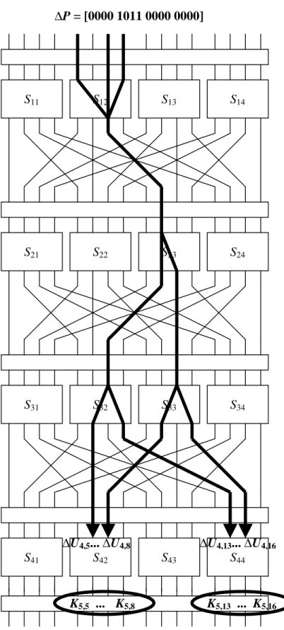
Once the linear approximation information has been compiled for the S-boxes in an SPN, we have the data to proceed with determining linear approximations of the overall cipher of the form of equation (1). This can be achieved by concatenating appropriate linear approximations of S-boxes. By constructing a linear approximation involving plaintext bits and data bits from the output of the second last round of S-boxes, it is possible to attack the cipher by recovering a subset of the subkey bits that follow the last round. We illustrate with an example.
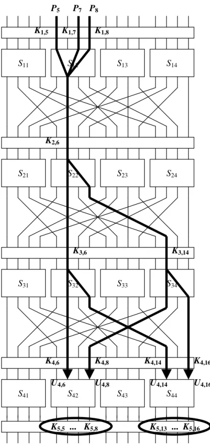
Consider an approximation involving S12, S22, S32, and S34 as illustrated in Figure 3. Note that this actually develops an expression for the first 3 rounds of the cipher and not the full 4 rounds. We shall see how this is useful in deriving the subkey bits after the last round in the next section.
We use the following approximations of the S-box:
S12: X1⊕X3⊕X4 = Y2 with probability 12/16 and bias +1/4 S22: X2 = Y2⊕Y4 with probability 4/16 and bias −1/4 S32: X2 = Y2⊕Y4 with probability 4/16 and bias −1/4 S34: X2 = Y2⊕Y4 with probability 4/16 and bias −1/4
Letting Ui (Vi) represent the 16-bit block of bits at the input (output) of the round i S- boxes and Ui,j (Vi,j) represent the j-th bit of block Ui (Vi) (where bits are numbered from 1 to 16 from left to right in the figure of the cipher). Similarly, let Ki represent the subkey block of bits exclusive-ORed at the input to round i, with the exception that K5 is the key exclusive-ORed at the output of round 4.
Hence, U1 = P ⊕ K1 where P represents the block of 16 plaintext bits and "⊕" represents the bit-wise exclusive-OR. Using the linear approximation of the 1st round, we then have
V1,6 = U1,5⊕ U1,7⊕ U1,8 (2)
= (P5 ⊕ K1,5) ⊕ (P7 ⊕ K1,7) ⊕ (P8 ⊕ K1,8) with probability 3/4. For the approximation in the 2nd round, we have
V2,6 ⊕ V2,8 = U2,6
with probability 1/4. Since U2,6 = V1,6 ⊕ K2,6, we can get an approximation of the form V2,6 ⊕ V2,8 = V1,6 ⊕ K2,6
K3,6 K2,6
K1,8 K1,7
K1,5
S21 S22 S23 S24
S11 S12 S13 S14
S31 S32 S33 S34
S41 S42 S43 S44
K4,8 K4,14 K4,16 K4,6
K3,14 P5 P7 P8
U4,6 U4,8 U4,14 U4,16
K5,5 ... K5,8 K5,13 ... K5,16
Figure 3. Sample Linear Approximation
with probability 1/4 and combining this with (2) which holds with probability of 3/4 gives
V2,6 ⊕ V2,8 ⊕ P5 ⊕ P7 ⊕ P8 ⊕ K1,5 ⊕ K1,7 ⊕ K1,8 ⊕ K2,6 = 0 (3) which holds with probability of 1/2 + 2(3/4−1/2)(1/4−1/2) = 3/8 (that is, with a bias of
−1/8) by application of the Piling-Up Lemma. Note that we are using the assumption that the approximations of S-boxes are independent which, although not strictly correct, works well in practice for most ciphers.
For round 3, we note that
V3,6 ⊕ V3,8 = U3,6
with probability 1/4 and
V3,14 ⊕ V3,16 = U3,14
with probability 1/4. Hence, since U3,6 = V2,6 ⊕ K3,6 and U3,14 =V2,8 ⊕ K3,14,
V3,6 ⊕ V3,8 ⊕ V3,14 ⊕ V3,16 ⊕ V2,6 ⊕ K3,6 ⊕ V2,8 ⊕ K3,14 = 0 (4) with probability of 1/2 + 2(1/4−1/2)2 = 5/8 (that is, with a bias of +1/8). Again, we have applied the Piling-Up Lemma.
Now combining (3) and (4), to incorporate all four S-box approximations, we get V3,6 ⊕ V3,8 ⊕ V3,14 ⊕ V3,16 ⊕ P5 ⊕ P7 ⊕ P8
⊕ K1,5 ⊕ K1,7 ⊕ K1,8 ⊕ K2,6 ⊕ K3,6 ⊕ K3,14 = 0.
Noting that U4,6 = V3,6 ⊕ K4,6, U4,8 = V3,14 ⊕ K4,8, U4,14 = V3,8 ⊕ K4,14, and U4,16 = V3,16 ⊕ K4,16, we can then write
U4,6 ⊕ U4,8 ⊕ U4,14 ⊕ U4,16 ⊕ P5 ⊕ P7 ⊕ P8 ⊕ ΣK = 0.
where
ΣK = K1,5 ⊕ K1,7 ⊕ K1,8 ⊕ K2,6 ⊕ K3,6 ⊕ K3,14 ⊕ K4,6 ⊕ K4,8 ⊕ K4,14 ⊕ K4,16
and ΣK is fixed at either 0 or 1 depending on the key of the cipher. By application of the Piling-Up Lemma, the above expression holds with probability 1/2+23(3/4−1/2)(1/4−1/2)3 = 15/32 (that is, with a bias of −1/32).
Now since ΣK is fixed, we note that
U4,6 ⊕ U4,8 ⊕ U4,14 ⊕ U4,16 ⊕ P5 ⊕ P7 ⊕ P8 = 0 (5) must hold with a probability of either 15/32 or (1−15/32) = 17/32, depending on whether ΣK = 0 or 1, respectively. In other words, we now have a linear approximation of the first three rounds of the cipher with a bias of magnitude 1/32. We must now discuss how such a bias can be used to determine some of the key bits.
3.5 Extracting Key Bits
Once an R−1 round linear approximation is discovered for a cipher of R rounds with a suitably large enough linear probability bias, it is conceivable to attack the cipher by recovering bits of the last subkey. In the case of our example cipher, it is possible to extract bits from subkey K5 given a 3 round linear approximation. We shall refer to the bits to be recovered from the last subkey as the target partial subkey. Specifically, the target partial subkey bits are the bits from the last subkey associated with the S-boxes in the last round influenced by the data bits involved in the linear approximation.
The process followed involves partially decrypting the last round of the cipher.
Specifically, for all possible values of the target partial subkey, the corresponding ciphertext bits are exclusive-ORed with the bits of the target partial subkey and the result is run backwards through the corresponding S-boxes. This is done for all known plaintext/ciphertext samples and a count is kept for each value of the target partial subkey. The count for a particular target partial subkey value is incremented when the linear expression holds true for the bits into the last round’s S-boxes (determined by the partial decryption) and the known plaintext bits. The target partial subkey value which has the count which differs the greatest from half the number of plaintext/ciphertext samples is assumed to represent the correct values of the target partial subkey bits. This works because it is assumed that the correct partial subkey value will result in the linear approximation holding with a probability significantly different from 1/2. (Whether it is above or below 1/2 depends on whether a linear or affine expression is the best approximation and this depends on the unknown values of the subkey bits implicitly involved in the linear expression.) An incorrect subkey is assumed to result in a relatively random guess at the bits entering the S-boxes of the last round and as a result, the linear expression will hold with a probability close to 1/2.
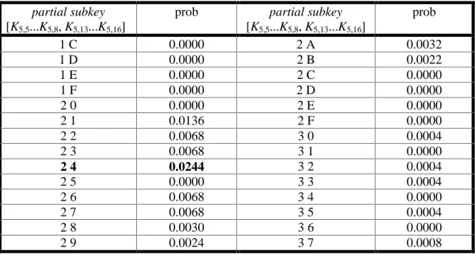
Let’s now put this into the context of our example. The linear expression of (5) affects the inputs to S-boxes S42 and S44 in the last round. For each plaintext/ciphertext sample, we would try all 256 values for the target partial subkey [K5,5...K5,8, K5,13...K5,16]. For each partial subkey value, we would increment the count whenever equation (5) holds true, where we determine the value of [U4,5...U4,8, U4,13...U4,16] by running the data backwards through the target partial subkey and S-boxes S24 and S44. The count which deviates the largest from half of the number of plaintext/ciphertext samples is assumed to the correct value. Whether the deviation is positive or negative will depend on the values of the subkey bits involved in ΣK. When ΣK = 0, the linear approximation of (5) will serve as the estimate (with probability < 1/2) and when ΣK = 1, (5) will hold with a probability > 1/2.
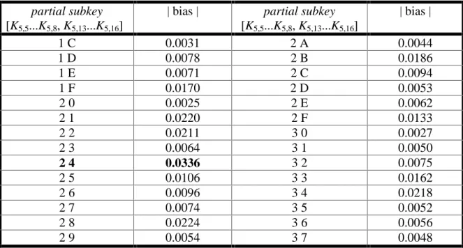
We have simulated attacking our basic cipher by generating 10000 known plaintext/ciphertext values and following the cryptanalytic process described for partial subkey values [K5,5...K5,8] = [0010] (hex 2) and [K5,13...K5,16] = [0100] (hex 4). As expected, the count which differed the most from 5000 corresponded to target partial subkey value [2,4]hex, confirming that the attack has successfully derived the subkey bits.
Table 5 highlights a partial summary of the data derived from the subkey counts. (The complete data involves 256 data entries, one for each target partial subkey value.) The values in the table indicate the bias magnitude derived from
| bias | = | count − 5000 | / 10000
where the count is the count corresponding to the particular partial subkey value.
As can be seen from the partial results in the table, the largest bias occurs for partial subkey value [K5,5...K5,8, K5,13...K5,16] = [2,4] and this observation was, in fact, found to be true for the complete set of partial subkey values.
partial subkey [K5,5...K5,8, K5,13...K5,16]
| bias | partial subkey [K5,5...K5,8, K5,13...K5,16]
| bias |
1 C 0.0031 2 A 0.0044
1 D 0.0078 2 B 0.0186
1 E 0.0071 2 C 0.0094
1 F 0.0170 2 D 0.0053
2 0 0.0025 2 E 0.0062
2 1 0.0220 2 F 0.0133
2 2 0.0211 3 0 0.0027
2 3 0.0064 3 1 0.0050
2 4 0.0336 3 2 0.0075
2 5 0.0106 3 3 0.0162
2 6 0.0096 3 4 0.0218
2 7 0.0074 3 5 0.0052
2 8 0.0224 3 6 0.0056
2 9 0.0054 3 7 0.0048
Table 5. Experimental Results for Linear Attack
The experimentally determined bias value of 0.0336 is very close to the expected value of 1/32 = 0.03125. Note that, although the correct target partial subkey has clearly the highest bias, other large bias values occur indicating that the examination of incorrect target partial subkeys is not precisely equivalent to comparing random data to a linear expression (where the bias could be expected to be very close to zero). Inconsistencies in the experimental biases can occur for several reasons including the S-box properties influencing the partial decryption for different partial subkey values, the imprecision of the independence assumption required for use in the Piling-Up Lemma, and the influence of linear hulls (to be discussed in the next section).
3.6 Complexity of Attack
We refer to the S-boxes involved in the linear approximation as active S-boxes. In Figure 3, the four S-boxes in rounds 1 to 3 influenced by the highlighted lines are active. The probability that a linear expression holds true is related to the linear probability bias in the active S-boxes and the number of active S-boxes. In general, the larger the magnitude of the bias in the S-boxes, the larger the magnitude of the bias of the overall expression.
Also, the fewer active S-boxes, the larger the magnitude of the overall linear expression bias.
Let ε represent the bias from 1/2 of the probability that the linear expression for the complete cipher holds. In his paper, Matsui shows that the number of known plaintexts required in the attack is proportional to ε−2 and, letting NL represent the number of known plaintexts required, it is reasonable to approximate NL by
NL ≈ 1/ε2.
In practice, it is generally reasonable to expect some small multiple of ε−2 known plaintexts are required. Although strictly speaking, the complexity of the cryptanalysis could be characterized in both time and space (or memory) domains, we refer to the data required to mount the attack when considering the complexity of the cryptanalysis. That is, we assume that if we are able to acquire NL plaintexts, we are able to process them.
Since the bias is derived using the Piling-Up Lemma where each term in the product refers to an S-box approximation, it is easy to see that the bias is dependent on the biases of the S-box linear approximations and the number of active S-boxes involved. General approaches to providing security against linear cryptanalysis have focused on optimizing the S-boxes (i.e., minimizing the largest bias) and finding structures to maximize the number of active S-boxes. The design principles of Rijndael are an excellent example of such an approach.
It must be cautioned, however, the concept of a "proof" of security to linear cryptanalysis is usually premised on the nonexistence of highly likely linear approximations. However, the computation of the probability of such linear approximations is based on the assumption that each S-box approximation is independent (so that the Piling-Up Lemma can be used) and on the assumption that one linear approximation scenario (i.e., a particular set of active S-boxes) is sufficient to determine the best linear expression between plaintext bits and data bits at the input to the last round. The reality is that the S- box approximations are not independent and this can have significant impact on the computation of the probability. Also, linear approximation scenarios involving the same plaintext and last round input bits but different sets of active S-boxes can combine to give a linear probability higher than that predicted by one set of active S-boxes. This concept is referred to as a linear hull [16]. Most notably for example, a number of linear approximation scenarios may have very small biases and on their own seem to imply that a cipher might be immune to a linear attack. However, when these scenarios are combined, the resulting linear expression of plaintext and last round input bits might have
a very high bias. Nevertheless, the approach outlined in this paper, tends to work well for many ciphers because the independence assumption is a reasonable approximation and when one linear approximation scenario of a particular set of active S-boxes has a high bias, it tends to dominate the linear hull.
4. Differential Cryptanalysis
In this section, we now turn our focus to the application of differential cryptanalysis to the basic SPN cipher.
4.1 Overview of Basic Attack
Differential cryptanalysis exploits the high probability of certain occurrences of plaintext differences and differences into the last round of the cipher. For example, consider a system with input X = [X1 X2 ... Xn] and output Y = [Y1 Y2 ... Yn]. Let two inputs to the system be X′ and X″ with the corresponding outputs Y′ and Y″, respectively. The input difference is given by ∆X = X′⊕ X″ where "⊕" represents a bit-wise exclusive-OR of the n-bit vectors and, hence,
] ...
[ X1 X2 Xn
X = ∆ ∆ ∆
∆
where ∆Xi = Xi′⊕Xi′′ with Xi′ and Xi″ representing the i-th bit of X′ and X″, respectively.
Similarly, ∆Y = Y′ ⊕ Y″ is the output difference and ] ...
[ Y1 Y2 Yn
Y = ∆ ∆ ∆
∆
where ∆Yi =Yi′⊕Yi′′.
In an ideally randomizing cipher, the probability that a particular output difference ∆Y occurs given a particular input difference ∆X is 1/2n where n is the number of bits of X.
Differential cryptanalysis seeks to exploit a scenario where a particular ∆Y occurs given a particular input difference ∆X with a very high probability pD (i.e., much greater than 1/2n). The pair (∆X, ∆Y) is referred to as a differential.
Differential cryptanalysis is a chosen plaintext attack, meaning that the attacker is able to select inputs and examine outputs in an attempt to derive the key. For differential cryptanalysis, the attacker will select pairs of inputs, X′ and X″, to satisfy a particular ∆X, knowing that for that ∆X value, a particular ∆Y value occurs with high probability.
In this paper, we investigate the construction of a differential (∆X, ∆Y) involving plaintext bits as represented by X and the input to the last round of the cipher as represented by Y. We shall do this by examining high likely differential characteristics where a differential characteristic is a sequence of input and output differences to the rounds so that the output difference from one round corresponds to the input difference for the next round. Using the highly likely differential characteristic gives us the opportunity to exploit information coming into the last round of the cipher to derive bits from the last layer of subkeys.
As with linear cryptanalysis, to construct highly likely differential characteristics, we examine the properties of individual S-boxes and use these properties to determine the
complete differential characteristic. Specifically, we consider the input and output differences of the S-boxes in order to determine a high probability difference pair.
Combining S-box difference pairs from round to round so that the nonzero output difference bits from one round correspond to the non-zero input difference bits of the next round, enables us to find a high probability differential consisting of the plaintext difference and the difference of the input to the last round. The subkey bits of the cipher end up disappearing from the difference expression because they are involved in both data sets and, hence, considering their influence on the difference involves exclusive- ORing subkey bits with themselves, the result of which is zero.
4.2 Analyzing the Cipher Components
We examine now the difference pairs of an S-box. Consider the 4×4 S-box representation of Figure 2 with input X = [X1 X2 X3 X4] and output Y = [Y1 Y2 Y3 Y4]. All difference pairs of an S-box, (∆X, ∆Y), can be examined and the probability of ∆Y given ∆X can be derived by considering input pairs (X′, X″) such that X′ ⊕ X″ = ∆X. Since the ordering of the pair is not relevant, for a 4×4 S-box we need only consider all 16 values for X′ and then the value of ∆X constrains the value of X″ to be X″ = X′ ⊕ ∆X.
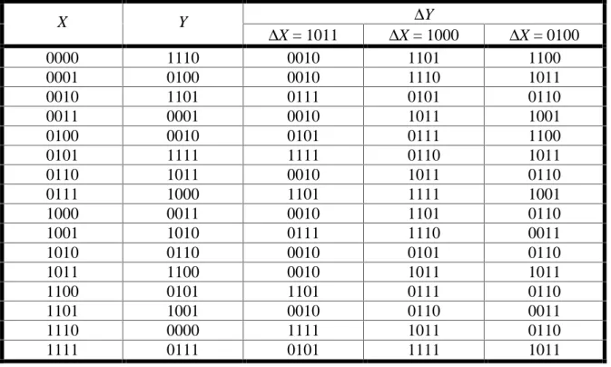
Considering the S-box of our cipher given in Section 2, we can derive the resulting values of ∆Y for each input pair (X′, X″=X′ ⊕ ∆X). For example, the binary values of X, Y, and the corresponding values for ∆Y for given input pairs (X, X ⊕ ∆X) are presented in Table 6 for ∆X values of 1011 (hex B), 1000 (hex 8), and 0100 (hex 4). The last three columns of the table represent ∆Y values for the value of X (as given by the row) and the particular
∆X value for each column. From the table, we can see that the number of occurrences of
∆Y = 0010 for ∆X = 1011 is 8 out of 16 possible values (i.e., a probability of 8/16); the number of occurrences of ∆Y = 1011 given ∆X = 1000 is 4 out of 16; the number of occurrences of ∆Y = 1010 given ∆X = 0100 is 0 out of 16. If the S-box could be "ideal", the number of occurrences of difference pair values would all be 1 to give a probability of 1/16 of the occurrence of a particular ∆Y value given ∆X. (It turns out that such an "ideal"
S-box is not mathematically possible.)
We can tabularize the complete data for an S-box in a difference distribution table in which the rows represent ∆X values (in hexadecimal) and the columns represent ∆Y values (in hexadecimal). The difference distribution table for the S-box of Table 1 is given in Table 7. Each element of the table represents the number of occurrences of the corresponding output difference ∆Y value given the input difference ∆X. Note that, besides the special case of (∆X = 0, ∆Y = 0), the largest value in the table is 8, corresponding to ∆X = B and ∆Y = 2. Hence, the probability that ∆Y = 2 given an arbitrary pair of input values that satisfy ∆X = B is 8/16. The smallest value in the table is 0 and occurs for many difference pairs. In this case, the probability of the ∆Y value occurring given the ∆X value is 0.
X Y ∆Y
∆X = 1011 ∆X = 1000 ∆X = 0100
0000 1110 0010 1101 1100
0001 0100 0010 1110 1011
0010 1101 0111 0101 0110
0011 0001 0010 1011 1001
0100 0010 0101 0111 1100
0101 1111 1111 0110 1011
0110 1011 0010 1011 0110
0111 1000 1101 1111 1001
1000 0011 0010 1101 0110
1001 1010 0111 1110 0011
1010 0110 0010 0101 0110
1011 1100 0010 1011 1011
1100 0101 1101 0111 0110
1101 1001 0010 0110 0011
1110 0000 1111 1011 0110
1111 0111 0101 1111 1011
Table 6. Sample Difference Pairs of the S-box
Output Difference
0 1 2 3 4 5 6 7 8 9 A B C D E F
0 16 0 0 0 0 0 0 0 0 0 0 0 0 0 0 0
1 0 0 0 2 0 0 0 2 0 2 4 0 4 2 0 0
2 0 0 0 2 0 6 2 2 0 2 0 0 0 0 2 0
3 0 0 2 0 2 0 0 0 0 4 2 0 2 0 0 4
4 0 0 0 2 0 0 6 0 0 2 0 4 2 0 0 0
5 0 4 0 0 0 2 2 0 0 0 4 0 2 0 0 2
6 0 0 0 4 0 4 0 0 0 0 0 0 2 2 2 2
7 0 0 2 2 2 0 2 0 0 2 2 0 0 0 0 4
8 0 0 0 0 0 0 2 2 0 0 0 4 0 4 2 2
9 0 2 0 0 2 0 0 4 2 0 2 2 2 0 0 0
A 0 2 2 0 0 0 0 0 6 0 0 2 0 0 4 0
B 0 0 8 0 0 2 0 2 0 0 0 0 0 2 0 2
C 0 2 0 0 2 2 2 0 0 0 0 2 0 6 0 0
D 0 4 0 0 0 0 0 4 2 0 2 0 2 0 2 0
E 0 0 2 4 2 0 0 0 6 0 0 0 0 0 2 0
I n p u t D
i f f e r e n c e
F 0 2 0 0 6 0 0 0 0 4 0 2 0 0 2 0
Table 7. Difference Distribution Table
There are several general properties of the difference distribution table that should be mentioned. First, it should be noted that the sum of all elements in a row is 2n =16;
similarly the sum of any column is 2n =16. Also, all element values are even: this results because a pair of input (or output) values represented as (X′, X″) has the same ∆X value as the pair (X″, X′) since ∆X = X′ ⊕ X″ = X″ ⊕ X′. As well, the input difference of ∆X = 0 must lead to an output difference of ∆Y = 0 for the one-to-one mapping of the S-box.
Hence, the top right corner of the table has a value of 2n = 16 and all other values in the first row and first column are 0. Finally, if we could construct an ideal S-box, which gives no differential information about the output given the input value, the S-box would have all elements in the table equal to 1 and the probability of occurrence of a particular value for ∆Y given a particular value of ∆X would be 1/2n = 1/16. However, as the properties discussed above must hold, this is clearly not achievable.
Before we proceed to discuss the combining of S-box difference pairs to derive a differential characteristic and an estimate of a good differential to use in the attack, we must discuss the influence of the key on the S-box differential. Consider Figure 4. The input to the "unkeyed" S-box is X and the output Y. However, in the cipher structure we must consider the keys applied at the input of each S-box. In this case, if we let the input to the "keyed" S-box be W = [W1 W2 W3 W4], we can consider the input difference to the keyed S-box to be
] ...
[W1 W1 W2 W2 Wn Wn
W = ′⊕ ′′ ′⊕ ′′ ′⊕ ′′
∆
where W′=[W1′ W2′...Wn′] and W′′=[W1′′ W2′′...Wn′′] represent the two input values.
Since the key bits remain the same for both W′ and W″,
∆Wi = Wi′ ⊕ Wi″ = (Xi′ ⊕ Ki) ⊕ (Xi″ ⊕ Ki)
= Xi′ ⊕ Xi″ = ∆Xi
since Ki⊕ Ki = 0. Hence, the key bits have no influence on the input difference value and can be ignored. In other words, the keyed S-box has the same difference distribution table as the unkeyed S-box.
X1 X2 X3 X4
4×4 S-box
K1
K2 K3
K4 W1 W2 W3 W4
Figure 4. Keyed S-box
4.3 Constructing Differential Characteristics
Once the differential information has been compiled for the S-boxes in an SPN, we have the data to proceed with determining a useful differential characteristic of the overall cipher. This can be done by concatenating appropriate difference pairs of S-boxes. By constructing a differential characteristic of certain S-box difference pairs in each round, such that a differential involves plaintexts bits and data bits to the input of the last round of S-boxes, it is possible to attack the cipher by recovering a subset of the subkey bits following the last round. We illustrate the construction of a differential characteristic with an example.
Consider a differential characteristic involving S12, S23, S32, and S33. As was the case for linear cryptanalysis, it is useful to visualize the differential characteristic in the form of a diagram as shown in Figure 5. The diagram illustrates the influence of non-zero differences in bits as they traverse the network, highlighting the S-boxes that may be considered as active (i.e., for which there is a non-zero differential). Note that this develops a differential characteristic for the first 3 rounds of the cipher and not the full 4 rounds. We shall see how this is useful in deriving bits from the last subkey in the next section.
We use the following difference pairs of the S-box:
S12: ∆X = B → ∆Y = 2 with probability 8/16 S23: ∆X = 4 → ∆Y = 6 with probability 6/16 S32: ∆X = 2 → ∆Y = 5 with probability 6/16 S33: ∆X = 2 → ∆Y = 5 with probability 6/16
All other S-boxes will have zero input difference and consequently zero output difference.
The input difference to the cipher is equivalent to the input difference to the first round and is given by
] 0000 0000 1011 0000
1 =[
∆
=
∆P U
where again, as with our presentation of linear cryptanalysis in Section 3, we are using Ui
to represent the input to the i-th round S-boxes and Vi to represent the output of the i-th round S-boxes. Hence, ∆Ui and ∆Vi represent the corresponding differences. As a result,
] 0000 0000 0010 0000
1 =[
∆V
considering the difference pair for S12 listed above and following the round 1 permutation ]
0000 0100 0000 0000
2 =[
∆U
S21 S22 S23 S24
S11 S12 S13 S14
S31 S32 S33 S34
S41 S42 S43 S44
∆U4,13... ∆U4,16
K5,5 ... K5,8 K5,13 ... K5,16
∆U4,5... ∆U4,8
∆P = [0000 1011 0000 0000]
Figure 5. Sample Differential Characteristic
with probability of 8/16 = 1/2 given the plaintext difference ∆P.
Now the second round differential using the difference pair for S23 results in ]
0000 0110 0000 0000
2 =[
∆V
and the permutation of round 2 gives
] 0000 0010 0010 0000
3 =[
∆U
with probability 6/16 given ∆U2 and a probability of 8/16 × 6/16 = 3/16 given ∆P. In determining the probability given plaintext difference ∆P, we have assumed that the differential of the first round is independent of the differential of the 2nd round and, hence, the probability of both occurring is determined by the product of the probabilities.
Subsequently, we can use the differences for the S-boxes of the third round, S32 and S33, and the permutation of the third round to arrive at
] 0000 0101 0101 0000
3 =[
∆V
and
] 0110 0000 0110 0000
4 =[
∆U (6)
with a probability of (6/16)2 given ∆U3 and, hence, a probability of 8/16 × 6/16 × (6/16)2
= 27/1024 given plaintext difference ∆P, where again we have assumed independence between the difference pairs of S-boxes in all rounds.
During the cryptanalysis process, many pairs of plaintexts for which ∆P = [0000 1011 0000 0000] will be encrypted. With high probability, 27/1024, the differential characteristic illustrated will occur. We term such pairs for ∆P as right pairs. Plaintext difference pairs for which the characteristic does not occur are referred to as wrong pairs.
4.4 Extracting Key Bits
Once an R−1 round differential characteristic is discovered for a cipher of R rounds with a suitably large enough probability, it is conceivable to attack the cipher by recovering bits from the last subkey. In the case of our example cipher, it is possible to extract bits from subkey K5. The process followed involves partially decrypting the last round of the cipher and examining the input to the last round to determine if a right pair has probably occurred. We shall refer to the subkey bits following the last round at the output of S- boxes in the last round influenced by non-zero differences in the differential output as the target partial subkey. A partial decryption of the last round would involve, for all S- boxes in the last round influenced by non-zero differences in the differential, the exclusive-OR of the ciphertext with the target partial subkey bits and running the data