A Note on Stochastic Volatility, GARCH models, and Hyperbolic Distributions

A Note on Stochastic Volatility, GARCH models, and Hyperbolic Distributions

Stefan R. Jaschke, December 13, 1997

We establish a relation between stochastic volatility models and the class of generalized hyperbolic distributions. These distribu- tions have been found to t exceptionally well to the empirical distribution of stock returns. We review the background of hyper- bolic distributions and prove stationary distributions of certain GARCH-type models to be generalized hyperbolic.

1 Introduction

The aim of this paper is to gather some results about the empirical distri- bution of stock returns and some attempts to match the heavy tails of these distributions in stochastic processes models, and to give an introduc- tory overview of the appearance of generalized hyperbolic distributions in this context.

There are some well-known empirical facts about log returns on stocks:

(i) The empirical distribution is leptokurtic compared to the normal dis- tribution.

(ii) Although there is no signicant serial correlation in stock returns, there is serial correlation in squared log returns.

Humboldt-Universitt Berlin, Institut fr Mathematik. The main part of the study of hyperbolic distributions and the research into stochastic volatility models was done when I was a guest at Aarhus University in 1994. As I continued to work in a dierent eld, the work never made it into a paper. During a discussion three years later I was encouraged to make a small note about the subject. I like to thank Uwe Kchler, Michael Srensen, and Rolf Tschernig for helpful comments on this paper. The note was nalized at the Sonderforschungsbereich 373 at Humboldt University Berlin. Financial support by the Deutsche Forschungsgemeinschaft is gratefully acknowledged.

1

Empirical and theoretical investigations of (i) have a long history. Mandel- brot and Fama proposed Pareto-stable distributions to explain the excess kurtosis in stock returns ((Fama 1965), (Mandelbrot and Taylor 1967)).

Mittnik and Rachev (1993) give an overview and comparison of alternative distributions in modeling stock returns. Evidence against stable Paretian distributions had been accumulated, and Mittnik and Rachev suggest the double Weibull-distribution for stock returns, whose density is

f⁽x ^{)= 1}

2

^jx^{j ;1exp (;}x ^{) (} >⁰ >⁰⁾:

One of their arguments in favor of the Weibull distribution is that tails de- crease exponentially. (They estimate to be close to 1.)

Hyperbolic distributions, which also have exponentially decreasing tails, were independently suggested as distributions of German stock returns by Eberlein and Keller (1994) and Kchler et al. (1994). (The logarithm of the density of a hyperbolic distribution is a hyperbola.) Hyperbolic distributions seem to t exceptionally well to the return in German stocks represented in the Stock index DAX. Barndor-Nielsen tted generalized hyperbolic distri- butions to Danish stock returns (Barndor-Nielsen 1994).

Let R^{k = log}S^{k ;log}S^k;1 denote the (one-period) log return, given a stock price process ⁽S^t)t201). Suppose that ⁽R^k) is stationary. We think that the important question now is what kind of stochastic process ⁽R^k) is, rather than looking at its marginal distributions only. Kchler et al. suggest

dX^{t =} m⁽X^t)dt⁺dW^t R^{n =} Xⁿ

m⁽x^{) = ;2}

2 (

x^;

q²⁺⁽x^{;)2 ;)}

m⁽x⁾ is chosen in such a way that the stationary distribution of X is hyperbolic. This approach is not satisfying for several reasons. First, a nontrivial m⁽x⁾ induces an autocorrelated series ⁽R^k) which is not what we observe. Second, in the continuous time version of the model, the stock price would be

S^{t=exp fZ t}

0

X^sds⁺t^g

which is absolutely continuous and of bounded variation. So, there would be arbitrage in the continuous-time option pricing theory (Harrison and Pliska 1981), if the locally riskless securityS^{t0 =exp fR0t}r^sds^gwasn't identical toS^t.

2

Lag

ACF

0 5 10 15 20 25

0.00.40.8

Series : dax

Lag

Partial ACF

5 10 15 20 25

-0.060.00.06

Series : dax

Lag

ACF

0 5 10 15 20 25

0.00.40.8

Series : dax2

Lag

Partial ACF

5 10 15 20 25

0.00.2

Series : dax2

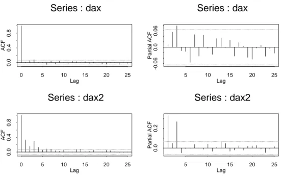
Figure 1: Autocorrelation in weekly log returns in the DAX 1974 1992 In this sense, the model proposed in (Kchler et al. 1994) is not suitable for the valuation of derivative securities.

Barndor-Nielsen (1994) suggests modeling ^logS^t with processes whose increments are independent and generalized hyperbolically distributed. Stock returns are, however, dependent, although there is no signicant linear depen- dence (serial correlation). The fact, that there is signicant serial correlation in squared residuals of many economic time series led to the development of stochastic volatility models, one important instance being the GARCH models.

Figure (1) shows the autocorrelation and partial autocorrelation of the weekly (log) return in the DAX and its square, respectively. The dotted line shows the level of signicance as given by the S-Plus function ^acf. All lags except the third show insignicant autocorrelation. Judging from both the autocorrelation function and the partial autocorrelation function, weekly DAX returns very much look like white noise. Looking at squared returns, however, signicant autocorrelation up to for weeks can be seen. There also seems to be some autocorrelation of squared returns at 13 weeks (a quarter of a year).

In section 2, we review some facts about generalized hyperbolic distri- butions and normal variance-mean mixtures. We show in section 3 that certain GARCH-type models produce stationary marginal distributions that

3

are generalized hyperbolic.

2 Generalized Hyperbolic Distributions as Nor- mal Variance-Mean Mixture Distributions

Hyperbolic distributions were introduced by Barndor-Nielsen (1977) in the context of the distribution of the size of sand particles taken from from the Danish coast. Plots of the log histogram of their log size seemed to have linear tails and could be very well tted by hyperbolae. This naturally led to the denition of the hyperbolic distribution, whose log density is a hyperbola:

logh⁽x ⁾⁼c^{(; q2+(}x^;)2+(x^;)): (1) (cis a norming constant,is a location parameter, a scale parameter, and

( +⁾x and ^{(; +)}x are the asymptotes of the hyperbola.)

Empirical distributions that apparently have exponentially decreasing tails abound. The examples given in Barndor-Nielsen (1977) include (log) diamond sizes from mining areas in South Africa, (log) personal income in Australia, and measurements of the velocity of light by Michelson.

There is a natural multivariate extension of (1) were the density is a hyper- boloid. It turns out that the marginal and conditional distributions of multi- variate hyperbolic distributions are not necessarily hyperbolic. Instead, hy- perbolic distributions can be embedded into the class of generalized hyperbolic distributions, which is invariant under margining , conditioning, and ane transformations. Many important distributions are in this class or a limit- ing case of it. Namely, the Gaussian distribution, Student's t-distribution, the Laplace-distribution, the gamma distribution, and the reciprocal gamma distribution. (See Barndor-Nielsen and Blaesild (1981)p.20].)

De nition (Barndor-Nielsen et al. 1982)

A random variable X ^{2 Rn} is said to be distributed according to a normal variance-mean mixture with location , drift , structure matrix , and mixing distribution F, if there is a random variable u with a distributionF on ⁰¹⁾ and the conditional distribution of X under u is normal:

P^{Xju =}Nⁿ⁽⁺uu⁾:

^2Rn,is symmetric and positive denite, ^{det ()=1}. We denote this distribution by NVMM⁽F⁾. (The condition^jj=1makes the choice of parameters unique and excludes the case ⁼⁰, where any distributionF

4

on ⁰¹⁾ could be written as NVMM⁽⁰¹⁰F⁾. For n ^{= 1}, the parameter

=1is irrelevant and we write NVMM⁽F⁾.)

If is the characteristic function of F, the characteristic function of NVMM⁽F⁾ is given by

⁽t⁾⁼e^{i<t> (}< t >⁺i

2

< tt >⁾ (2) as is easily seen. A simple consequence of (2) is that the sum of i.i.d. NVMM variables with the same and is again a NVMM distribution:

NV MM⁽F^{)n =}NV MM⁽nFⁿ⁾:

Furthermore, this class of mixtures is closed under margining, conditioning and ane transformations. Details are given in (Barndor-Nielsen et al.

1982, p.147).

Generalized hyperbolic distributionscan now be dened as normal variance- mean mixtures were the mixing distribution is a generalized inverse Gaussian distribution N^;()that is dened by having the following density:

f⁽x^{)= (}=⁾⁼²

2K^(p)x^{;1exp f;1}

2

(x^;1+x^)g: ⁽x >⁰⁾

(K is a Bessel function. The parameter domain is ^{2 R}, > ⁰, > ⁰. Additionally,⁼⁰is allowed for >⁰ and ⁼⁰is allowed for <⁰.) Let

H^{( ) =} NV MM⁽N^{;(22)) 2 = 2;}< >

denote the generalized hyperbolic distribution. The density and char- acteristic function of the generalized hyperbolic distribution are given in Barndor-Nielsen et al. (1982)p.148]. For ⁼⁽n⁺¹⁾=², the density simpli- es to

(=⁾

(2^);12 K⁽⁾e^{; p2+<x;;1}(x;)>+<x;>

whose logarithm is a hyperboloid in x.

Maximum likelihood estimation for hyperbolic distributions with param- eters H^{(1 )} is discussed in Barndor-Nielsen and Blaesild (1981), where it is noted that the computation of the MLE is "from a theoretical as well as from a computational point of view rather unpleasant", p.29].

Namely, the log-likelihood function may have saddle points.

5

Back to the feature that gave rise to the denition of the hyperbolic distribution. It is shown in Barndor-Nielsen and Blaesild (1981)pp.34] that for the density h of the univariate generalized hyperbolic distribution

h⁽x ^=0)jx^j;1e^{;( ;)x} as x^!1

for >⁰. It is dubious whether one can see the eect of the power ^jx^j;1 in the log histogram. That is, generalized hyperbolic distributions very much look like hyperbolic distributions in the tails. That so much is known about generalized hyperbolic distributions makes it worthwhile investigat- ing whether normal variance-mean mixture distributions implied by certain stochastic models are in fact generalized hyperbolic.

3 Normal Variance-Mean Mixture Distributions Generated by Stochastic Processes

If W is a one-dimensional Wiener-process and is an independent random time with distribution F, then

^{+ +}W NVMM⁽F⁾:

Moreover, if ^fag is an increasing stochastic process which is independent of W, then X^{a := +a+}W^a is a stochastic process whose increments are mixed normal. For nancial markets, a ^{! a} can be thought of as a random time change mapping calendar time to internal market time or operational time. The generalized hyperbolic distribution with ^{= ;12} is now naturally obtained by letting ^a be a certain rst hitting time of an independent Wiener-process B:

^a:=inf

t0

ft⁺B^t a^g:

^a is a Levy-process, i.e. it has independent increments. The increments are inverse Gaussian distributed: ^{b ;a} N^;(;12((b^;a⁾⁾²²⁾. Now, X^{a =}W ^a is a Levy-process with generalized hyperbolic increments. X was termed Gaussian-inverse Gaussian process and its Levy decomposition was given by Barndor-Nielsen (1994). X is a pure jump process, and the Levy measure is not integrable at 0. That means, X has innitely many (small) jumps in any time interval. X can be thought of as a limit of compound Poisson processes.

6

Normal variance-mean mixtures also appear in stochastic volatility mod- els were log returns are conditionally on some stochastic volatility multivariate Gaussian:

R^k=+k2+kz^k:

is a stochastic process and z^k is Gaussian white noise (z^k i.i.d. N^{n(0) 2 Rn}). If ² is a stationary process with marginal distribution F and independent of⁽z^k), thenRis a stationary process with marginal distribution NVMM⁽F⁾.

One simple example of a stochastic model forr^t:=2t is

dr^{t =(}!^;r^t)dt⁺cr^tdW^t (3) where W^t is an independent Wiener-process. In the framework of Nelson (1990), (3) is a weak limit of the volatility process in the GARCH(1,1)-model

r^{(k+1)h =}!^h+r^kh(h+c^hB^{kh2 )}

for h ^{! 0}, and B^kh i.i.d.N⁽⁰h⁾, !^{h =} !h, ^{h = 1;}c^qh=^2;h, c^{h =} c=^p2h. Nelson (1990) shows that the stationary distribution of (3) is recipro- cal gamma if¹⁺²=c²>⁰and! >⁰. That is, if¹=r^{0 ;(1+2}=c²²!=c²⁾, then r is (strictly) stationary.¹ Now, the stationary distribution ofR is gen- eralized hyperbolic H^(;(1+2=c^2)2p!=c⁾. (Note that this one has tails ^jx^j;1 for x ^{! 1} and e^2x for x ^{! ;1} which is not quite what we observe.)

Yet another simple volatility model is dr^{t =(}!^;r^t)dt⁺c^pr^tdW^t:

Its stationary distribution is a gamma distribution: ^;(2!=c²²=c²⁾. Hence, the stationary distribution of R is generalized hyperbolic with parameters H⁽²!=c^2q4=c²⁺²⁰⁾.

4 Conclusion

(i) For stock returns, Gaussian tails ( e^;x2) are too light while Pareto- stable tails ( ^jx^j ) seem to be too heavy. The tails of generalized hyperbolic distributions ( ^jx^j e^;x) which Barndor-Nielsen calls semi-heavy seem to t just right to the distribution of (log) stock returns.

1Let ^{;( b)} denote the gamma distribution with density ^{(b =;( ))x ;1e;bx}, ^{x > 0}. Then^{;( b)=N;( 02b)}and, if^{X;( b)}, then^{X;1N;(; 2b0)}.

7

(ii) Many stochastic volatility models produce almost by denition log returns whose stationary distribution is a normal variance-mean mixture. As the subclass of generalized hyperbolic distributions has several nice properties and is well-studied, it is worthwhile to investigate whether new (or old) stochastic volatility models produce log returns that are in fact generalized hyperbolic.

References

Barndor-Nielsen, O. (1977). Exponentially decreasing distributions for the logarithm of particle size, Proc. R. Soc. London A ³⁵³: 401419.

Barndor-Nielsen, O. (1994). Gaussian-inverse Gaussian processes and the modelling of stock returns, presented at the 2. Workshop on Stochastics and Finance 1994 in Berlin.

Barndor-Nielsen, O. and Blaesild, P. (1981). Hyperbolic distributions and ramications: Contributions to theory and application, in C. T. et al. (ed.), Statistical Distributions in Scientic Work, Vol. 4, D. Reidel Publishing Company, pp. 1944.

Barndor-Nielsen, O., Kent, J. and Srensen, M. (1982). Normal variance- mean mixtures and z distributions, International Statistical Review

50: 145159.

Eberlein, E. and Keller, U. (1994). Hyperbolic distributions in nance, Re- search report, Institut fr Mathematische Stochastik, Universitt Freiburg.

presented at the 2. Workshop on Stochastics and Finance 1994 in Berlin.

Fama, E. (1965). The behavior of stock market prices, Journal of Business

38: 34105.

Harrison, J. and Pliska, S. (1981). Martingales and stochastic integrals in the theory of continuous trading, Stochastic Processes and Applications

11: 215260.

Kchler, U., Neumann, K., Srensen, M. and Streller, A. (1994). Stock re- turns and hyperbolic distributions, Discussion Paper 23, Sonderforschungs- bereich 373, Humboldt-Universitt zu Berlin. presented at the 2. Workshop on Stochastics and Finance 1994 in Berlin.

Mahieu, R. J. (1995). Financial Market Volatility, Universitaire Pers Maas- tricht.

8

Mandelbrot, B. and Taylor, H. (1967). On the distribution of stock price dierences, Operations Research¹⁵: 1057+.

Mittnik, S. and Rachev, S. (1993). Modeling asset returns with alternative stable distributions, Econometric Reviews ¹²(3): 261330.

Nelson, D. B. (1990). ARCH models as diusion approximations, Journal of Econometrics ⁴⁵: 738.

9