An experimental analysis of German farmers’ decisions to buy or rent farmland

Published by

DFG Research Unit 2569 FORLand, Humboldt-Universität zu Berlin Unter den Linden 6, D-10099 Berlin

https://www.forland.hu-berlin.de

Tel +49 (30) 2093 46845, Email gabriele.wuerth@agrar.hu-berlin.de

A gr icul tur al Land M ar ket s – E ffici ency and R egul ati on

An experimental analysis of German farmers’ decisions to

buy or rent farmland

Matthias Buchholz, Michael Danne and Oliver Musshoff

FORLand-Working Paper 18 (2020)

An experimental analysis of German farmers’

decisions to buy or rent farmland

Matthias Buchholz

, Michael Danne

, Oliver Musshoff

January 2020

Abstract

Farmland is an essential agricultural production factor that farmers can choose to either buy or rent. In this paper, we apply a discrete choice experiment to analyse German farmers’ individual buying and rental decisions for farmland. Our results reveal that farmers have a higher willingness to buy than to rent farmland. Covariates such as farmers’ risk attitude affect the decisions in the discrete choice experiment while no effect was observable for individual expectations about future farmland prices. Direct payments considerably raise farmers’ willingness to buy and rent farmland. Farmers’ decisions deviate substantially from normative predictions from the present value model.

Keywords: Agricultural Land Market, Farmland, Rent-or-Buy Decision, Discrete Choice Experiment, Present Value Model

JEL codes: C93, D90, Q10 Acknowledgements

Financial support from the German Research Foundation (DFG) through Research Unit 2569

“Agricultural Land Markets – Efficiency and Regulation” is gratefully acknowledged.

∗ Matthias Buchholz, matthias.buchholz@agr.uni-goettingen.de

∗∗ Michael Danne, michael.danne@agr.uni-goettingen.de

∗∗∗ Oliver Musshoff, oliver.musshoff@agr.uni-goettingen.de

1

Farmland is an essential asset for agricultural production. While farmland is scarce, farmers can usually decide to either buy or rent farmland. Although the analysis of farmland prices and rental rates has a long tradition in agricultural economics, the recent boost in farmland prices and rental rates in large parts of the world and, particularly in Germany, has renewed interest in this strand of research among academics and policymakers alike (Breustedt and Habermann, 2011; Croonenbroeck, Odening and Hüttel, 2019; Graubner, 2018; Hennig and Latacz-Lohmann, 2016; Lehn and Bahrs, 2018; März et al., 2016).

From 2003 to 2016, farmland prices and rental rates in Germany surged, on average, from 9,184 €/ha to 22,310 €/ha (+142.92 %) and 174 €/ha to 288 €/ha (+65.52 %), respectively (Bundesministerium für Ernährung und Landwirtschaft, 2017). However, there is no consensus regarding whether price developments of farmland and rental rates can be explained or predicted by normative theory which has implications for policy advice. According to the present value model (PVM), farmland prices should equal the discounted stream of expected agricultural returns. In empirical research on farmland prices, agricultural returns are commonly approximated by rental rates establishing a direct link between farmland prices and rental rates (Robison, Lins and VenKataraman, 1985). Thus, farmland prices and rental rates should be cointegrated (Gutierrez, Westerlund and Erickson, 2007; Nickerson and Zhang, 2014). However, it appears that the PVM might fail. In other words, there is a discrepancy between empirically observed and expected farmland values (Hanson and Myers, 1995).

Using historical time series data for farmland prices and rental rates, Clark, Fulton and Scott (1993) show that land prices rise and fall faster than rental rates, an observation which challenges the fundamental assumption of the PVM. It seems reasonable that farmland prices and rental rates are determined by pure economic factors such as expected cash flows, interest rates, soil quality, plot size, livestock density or the portion of high value crops grown, for instance (Hennig and Latacz-Lohmann, 2016; Hüttel et al., 2013; Lehn and Bahrs, 2018;

März et al., 2016). Nevertheless, the reasons for the empirical rejection of the PVM and the determinants that influence farmers’ decisions to either buy or rent farmland are not clear.

From a methodological perspective, econometric approaches almost exclusively constitute the basis for the analysis of farmland prices and rental rates. In particular, hedonic pricing models have been widely applied to address multiple research questions in the context of farmland markets (Borchers, Ifft and Kuethe, 2014; Nickerson and Zhang, 2014). These studies are usually based on reported farmland prices or rental rates which do not reveal explanations for a deviation from normative predictions that might, e.g., result from confounding sociodemographic characteristics not available in official statistics. A joint analysis of farmland prices and rental rates is made more difficult by the fact that reported figures are usually not available for the same plot of land leading to a missing counterfactual problem (e.g. Pufahl and Weiss, 2009). While the roles of individual attitudes, multiple goals and bounded rationality in farmer decision-making have gained much attention in the field of agricultural economics in recent years (Bocquého, Jacquet and Reynaud, 2013; Dessart, Barreiro-Hurlé and van Bavel, 2019), comparable analyses for agricultural land markets do not exist. For instance, there is no empirical evidence on how farmers’ risk aversion could affect the willingness to pay (WTP) for farmland available.

In this regard, the application of economic experiments might be a promising approach to enhance the understanding of farmland prices and rental rates while taking individual decisions and attitudes of farmers as well as sociodemographic characteristics not available in official statistics into account. Generally, the analysis of land markets by means of economic experiments is a novel field of research. Duke and Gao (2018) carried out a first laboratory experiment with business and economics students to investigate how different property taxation regimes affect land investments in the housing sector. According to the authors, diverging results from the experiment and from simulated optimal predictions under utility- maximization may provide insights about difficulties regarding land tax efficiency and acceptability.

(1) With this in mind, we conduct a discrete choice experiment (DCE) with German farmers and seek to address the following research questions:

(2) Do the farmers in the DCE prefer to buy or rent the offered parcels of farmland?

(3) How do the attributes ‘gross margin’ generated, ‘interest rate’ and magnitude of the ‘direct payments’ drive farmers’ WTP for buying or renting farmland?

(4) Do reported sociodemographic / farm characteristics and individual price expectations affect buying or rental decisions?

(5) Are farmers’ buying or rental decisions in line with normative expectations predicted by the PVM?

To the best of our knowledge, this is the first experimental study that analyses farmers’

individual buying and rental decisions for farmland. In each choice decision of the DCE, farmers can buy land, rent land or choose an opt-out option. For each choice situation, we conduct a normative benchmark comparison based on the PVM.

The remainder of this study is organised as follows: In Section 2, we explain the experimental design. In Section 3, we present methods applied for data analysis. Section 4 reports results followed by our conclusions and prospects for future research in Section 5.

2

The experiment consists of four parts and was structured as follows: First, participants were asked to provide operational farm characteristics. Second, the DCE was conducted. Third, we asked farmers about the current situation on the regional land market and the expected development of future farmland prices and rental rates. Finally, sociodemographic characteristics and the self-assessed risk-attitude following Dohmen et al. (2011) were collected.

2.1 The discrete choice experiment

Usually, there is no data available on how farmers choose to buy or rent the same parcel of farmland. Under these conditions, DCEs are well-suited to reveal the preferences of German farmers for either buying or renting farmland. DCEs are based on the stated preference approach. Based on hypothetical choice situations in the experiment, researchers are able to derive preferences for real choice decisions that have not been articulated before or for which

respondents’ preferences is possible through a scenario of hypothetical decision-making situations (List, Sinha and Taylor, 2006). In a DCE, participants are confronted with a number of choice sets consisting of different alternatives and are asked to select one of the given alternatives. Each presented alternative is characterized by pre-defined attributes and associated levels. By systematically varying the levels of the attributes, the respective influence on choice decisions can be determined (Louviere et al., 2000) .

The DCE in this study entails the following decision situation: the farmers had to choose either to buy or to rent farmland or to reject both of these options (opt-out). The opt-out alternative was included because the acquisition of additional farmland is voluntary. A forced choice could lead to inaccuracy and inconsistency in terms of demand theory (Hanley, Ryan and Wright, 2003). In each decision situation, the choice to buy or to rent farmland was described by the following attributes: purchase price / rental rate, interest rate, gross margin and direct payments. The attributes and levels used in the experiment are shown in Table 1.

Table 1. Attributes and levels in the DCE.

Attributes Levels

Purchase price 10,000 €/ha; 20,000 €/ha; 30,000 €/ha; 40,000 €/ha; 50,000 €/ha Rental rate 200 €/ha; 400 €/ha; 600 €/ha; 800 €/ha; 1,000 €/ha

Interest rate 1 %; 3 %; 5 %; 7 %

Gross margin 200 €/ha; 400 €/ha; 600 €/ha; 800 €/ha; 1,000 €/ha Direct payments 0 €/ha; 90 €/ha; 180 €/ha; 270 €/ha

Source: Author`s own illustration

To reduce the complexity of the experiment, selection of the attributes is based on pragmatic reasoning and relevance for agricultural land markets. Levels for attributes were determined so as to cover a realistic range of actual and past values farmers are familiar with. In addition, helpful advice from experts and suggestions from a comprehensive pre-test with farmers were used to calibrate attribute levels. Moreover, consideration of the attribute ‘direct payments’

allows us to contrast the effects of direct payments on farmland prices and rental rates found in the experiment with existing evidence from econometric models available in a rich body of literature on this topic (Guastella et al., 2018; Ifft, Kuethe and Morehart, 2015; Michalek, Ciaian and Kancs, 2014). In doing so, we can test the suitability of our experimental approach for an ex-ante analysis of amended agricultural policies.

The DCE is comprised of two alternatives and five attributes, resulting in a full-factorial design of 2,000 possible decision situations or choice sets. To ensure applicability for farmers, the number of choice sets was reduced by means of a so-called ‘efficient design’. Efficient designs allow for the consideration of ex ante information and the associated uncertainty in terms of random distributions regarding the population’s utility parameters. In such designs, prior parameter estimates are drawn from Bayesian parameter distributions and are therefore known as Bayesian or D-efficient designs (Rose and Bliemer, 2009). Preliminary data for our final design was collected in a pilot study with 14 farmers. The D-error is used as efficiency criterion for the efficient design as it considers the minimization of the standard errors and the covariance of the estimated utility parameters. Based on the preliminary data, a D-efficient

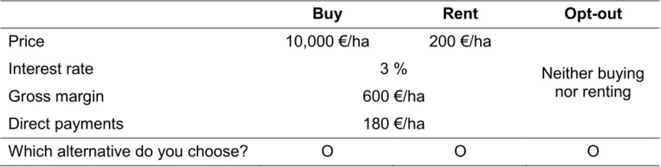
Bayesian design (D-error of 0.020) was created using the software Ngene 1.1.2. As a result, the number of choice sets was reduced to 15 which were then presented to the farmers in randomised order. As an example, Table 2 displays one of the 15 choice sets.

Table 2. Example choice set.

Buy Rent Opt-out

Price 10,000 €/ha 200 €/ha

Neither buying nor renting

Interest rate 3 %

Gross margin 600 €/ha

Direct payments 180 €/ha

Which alternative do you choose? O O O

Source: Author`s own illustration

To ensure that farmers understood the experiment, we provided detailed instructions at the beginning of the experiment in which all attributes and their levels were explained. Following these instructions, control questions were asked to explicitly test if the participant understood the instructions. These questions are designed in such a way that correct answers were required in order to proceed. Moreover, the description of the attributes remained available to participants throughout the whole experiment by means of ‘mouse over buttons’ in each choice set. In doing so, we ensured that the chosen attributes and levels were understood, and explanations were available during the whole experiment.

2.2 Data collection

For the empirical analysis, primary data was collected from German farmers. An anonymous online survey was developed and available to participants from the end of January to the beginning of March 2019. Farmers were invited to participate in the survey through a mailing list comprising e-mail addresses of farmers who have participated in previous surveys and who have agreed to participate again. Moreover, links to the experiment were available in newsletters of regional farmers’ associations and social media channels. To further incentivise farmer participation, each of the participants received a compensation of € 10 upon completion of the experiment. Based on a comprehensive pre-test, the expected time to finish the experiment was 20 minutes. Furthermore, we provided additional cash prizes to enhance motivation for careful decisions in the experiment. Five farmers were randomly selected, each of whom received a prize of €100.

In total, 443 participants opened the link to start the experiment of which 29 % quit immediately after reading the first page, an additional share of 23 % quit during the experiment and 48 % of the participants completed the experiment successfully. Nine out of 213 participants provided implausible information and were removed from the data set. Ultimately, the decisions and reported answers of 204 farmers were included in the analysis.

3

3.1 Econometric analysis of the choice model

According to random utility theory (Luce, 1959; McFadden, 1974), the utility 𝑈𝑈 of an individual n from choosing an alternative s is divided into a deterministic component V and an independent and identically distributed (IID) random component ɛ_{𝑠𝑠𝑠𝑠} (Hensher, Rose and Greene, 2015). With 𝑥𝑥_{𝑠𝑠𝑠𝑠} as a vector of attributes and socioeconomic characteristics of n, and 𝛽𝛽_𝑠𝑠 as a vector of individual parameters associated with 𝑥𝑥_{𝑠𝑠𝑠𝑠}. The utility function for individual n for choosing an alternative s is:

𝑈𝑈_{𝑠𝑠𝑠𝑠} = 𝑉𝑉_{𝑠𝑠𝑠𝑠} + ɛ_{𝑠𝑠𝑠𝑠}=𝛽𝛽_𝑠𝑠𝑥𝑥_{𝑠𝑠𝑠𝑠}+ ɛ_{𝑠𝑠𝑠𝑠} (1) An individual n chooses the alternative for which he or she has the highest preferences. Under the assumption of utility maximization, the probability 𝑃𝑃_{𝑠𝑠𝑠𝑠} that an individual n chooses alternative s instead of j from a finite set of choices 𝐶𝐶_𝑠𝑠 is:

𝑃𝑃_{𝑠𝑠𝑠𝑠}=𝑃𝑃𝑃𝑃𝑃𝑃𝑃𝑃�𝑈𝑈𝑠𝑠𝑠𝑠>𝑈𝑈_{𝑗𝑗𝑠𝑠}� ∀ 𝑗𝑗 𝜖𝜖 𝐶𝐶_𝑠𝑠,𝑠𝑠 ≠ 𝑗𝑗 (2)

In our analysis, we apply a mixed logit model. The mixed logit model, also referred to as random parameter model, is able to account for random taste variation which means that individuals have different βs. Hence, preference heterogeneity may be considered in the estimation process (Train, 2009; Hensher, Rose and Greene, 2015). In mixed logit models, the utility parameters 𝛽𝛽_𝑠𝑠 vary randomly across the sample population (Hensher, Rose and Greene, 2015). The choice probability in the mixed logit model is:

The panel-structure of the data set should be considered in the estimation process (Train, 2009). Therefore, the random parameters are held constant over choice situations. Thus, equation (3) becomes:

𝑃𝑃_{𝑠𝑠𝑠𝑠}=� �� 𝑒𝑒𝑥𝑥𝑝𝑝(𝛽𝛽_𝑠𝑠𝑥𝑥𝑠𝑠𝑠𝑠𝑛𝑛)

∑ 𝑒𝑒𝑥𝑥𝑝𝑝(𝛽𝛽_𝑠𝑠 𝑠𝑠𝑥𝑥𝑠𝑠𝑠𝑠𝑛𝑛)

𝑛𝑛 �

𝛽𝛽

𝑓𝑓(𝛽𝛽)𝑑𝑑(𝛽𝛽) (4)

where t = 1,…,T contains the number of choice situations. The integral in equation (4) has no closed form and cannot be calculated exactly. Thus, the choice probability is approximated through simulation of log-likelihood functions 𝐿𝐿𝐿𝐿_𝑠𝑠 determined by R simulation runs:

𝐿𝐿𝐿𝐿𝑠𝑠 = � 𝑙𝑙𝑙𝑙1

𝑅𝑅 � �

𝑒𝑒𝑥𝑥𝑝𝑝(𝛽𝛽´_𝑠𝑠𝑥𝑥_{𝑠𝑠𝑠𝑠𝑛𝑛})

∑ 𝑒𝑒𝑥𝑥𝑝𝑝(𝛽𝛽´_{𝑠𝑠 𝑠𝑠}𝑥𝑥_{𝑠𝑠𝑠𝑠𝑛𝑛})

𝑛𝑛 𝑟𝑟

𝑠𝑠 (5)

𝑃𝑃𝑠𝑠𝑠𝑠=� � 𝑒𝑒𝑥𝑥𝑝𝑝(𝛽𝛽_𝑠𝑠𝑥𝑥_{𝑠𝑠𝑠𝑠})

∑ 𝑒𝑒𝑥𝑥𝑝𝑝(𝛽𝛽_𝑖𝑖 𝑠𝑠𝑥𝑥𝑠𝑠𝑠𝑠)�

𝛽𝛽

𝑓𝑓(𝛽𝛽)𝑑𝑑(𝛽𝛽) (3)

In order to consider the heterogeneity in preferences within mixed logit models, it is necessary to enter individual specific attributes via interaction terms in the model estimation process (Boxall and Adamowicz, 2002; Hanley, Ryan and Wright, 2003).

The marginal WTP for an attribute is computed by dividing the estimated attribute parameter of the variable in question by the estimated attribute parameter of the monetary variable (Hu et al., 2012; Schulz, Breustedt and Latacz-Lohmann, 2014).

𝑊𝑊𝑊𝑊𝑃𝑃_{𝑋𝑋𝑘𝑘} =−_𝛽𝛽^{𝛽𝛽𝑘𝑘}

𝑃𝑃, (6)

where 𝛽𝛽_𝑘𝑘 and 𝛽𝛽_𝑃𝑃 are the estimated coefficients of the attributes 𝑋𝑋_𝑘𝑘 and the price P. We kept the parameters of the price attributes fixed (Das, Anderson and Swallow, 2009; Lancsar, Fiebig and Hole, 2017). The WTP values and their confidence intervals were derived by means of the Krinsky and Robb method using the Stata module wtp (Hole, 2007) with 10,000 replications.

3.2 Derivation of the present value model (normative benchmark)

In the DCE, participating farmers have to decide if they would like to use additional farmland for agricultural production. There are 𝑆𝑆= 3 decision alternatives (𝐴𝐴_𝑠𝑠): (i) purchasing farmland, (ii) renting farmland and (iii) no additional use of farmland (opt-out). A pure profit-maximizing decision-maker will choose the alternative 𝑠𝑠 which generates the highest present value (𝑃𝑃𝑉𝑉) of the returns from additional farmland:

max𝐴𝐴_𝑠𝑠 𝑃𝑃𝑉𝑉(𝐴𝐴_𝑠𝑠) (7)

To calculate the present value of the returns from each decision alternative, we have to take the different attributes and their levels which are given in the DCE into account: The purchase price (𝑃𝑃𝑃𝑃 ) and the annual rental rate (𝑅𝑅𝑅𝑅 ) for farmland as well as the interest rate (𝑖𝑖 ).

Furthermore, the average expected gross margin per land unit (𝐺𝐺𝐺𝐺) and the average expected direct payments (𝐷𝐷𝑃𝑃) over a time horizon of 𝑊𝑊= 10 years are given in the DCE. Moreover, we asked each participating farmer about the expected development of farmland prices over the next ten years. The expected price development can be interpreted as a growth rate for farmland prices 𝑃𝑃 . For the purchase alternative, we can calculate the present value of the returns:

𝑃𝑃𝑉𝑉(𝐴𝐴𝑝𝑝𝑝𝑝𝑟𝑟𝑝𝑝ℎ𝑎𝑎𝑠𝑠𝑎𝑎) =−𝑃𝑃𝑃𝑃+ (𝐺𝐺𝐺𝐺+𝐷𝐷𝑃𝑃)∙ 𝐶𝐶𝐶𝐶_{𝑖𝑖,𝑇𝑇}+𝑃𝑃𝑃𝑃 ∙(1 +𝑃𝑃)∙(1 +𝑖𝑖)^−𝑇𝑇 (8)

𝐶𝐶𝐶𝐶_{𝑖𝑖,𝑇𝑇} denotes the capitalization factor given the interest rate 𝑖𝑖 and the considered time horizon

𝑊𝑊. For the rental alternative, the present value of the returns of additional land can be calculated as follows:

𝑃𝑃𝑉𝑉(𝐴𝐴_{𝑟𝑟𝑎𝑎𝑠𝑠𝑛𝑛}) = (−𝑅𝑅𝑅𝑅+𝐺𝐺𝐺𝐺+𝐷𝐷𝑃𝑃)∙ 𝐶𝐶𝐶𝐶_{𝑖𝑖,𝑇𝑇} (9)

The payoff from not using additional land (opt-out) is zero:

𝑃𝑃𝑉𝑉(𝐴𝐴𝑜𝑜𝑝𝑝𝑛𝑛−𝑜𝑜𝑝𝑝𝑛𝑛) = 0 (10)

On the one hand, we can derive the alternative which maximizes the utility of a pure profit- maximizing decision maker (normative benchmark). On the other hand, we observe the decision alternative which was selected by the participant in the DCE. Finally, we can compare the normative benchmark with the decisions observed in the experiment. In doing so, we can answer the question whether a decision-maker decides in accordance with a pure profit- maximizing decision maker or if considerable deviations occur.

4

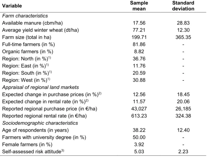
4.1 Sample description and individual appraisal of regional land markets Table 3 reports the farm and sociodemographic characteristics of the participating farmers and their reported appraisal of regional land markets. Generally, the standard deviations indicate substantial variation within the sample of farmers which may also influence the results from the DCE. On average, the total area of the farms comprises 199.71 ha for which 17.56 cubic meter manure per ha is available.

81.86 % of the participants are full-time farmers and 8.82 % manage their farms organically.

The average yield for winter wheat as the most prominent crop in Germany is 77.21 dt/ha.

Farmers are located throughout all regions of Germany. Furthermore, the reported average regional purchase price for farmland in recent years is 43,027 €/ha. The reported rental rate for new contracts closed recently amounts to 613.23 €/ha in our sample. On average, farmers expect farmland prices and rental rates to rise by 12.56 % and 11.57 % in the next 10 years to come. On average, the farmers are 38.22 years old. The share of female farmers amounts to 3.92 % and 50.00 % of all the respondents graduated from university. The relatively high share of farmers with a university degree might result from the fact that we generated our sample using an online experiment. While online experiments have great advantages, due to the low costs and easy acquisition of potential participants, it appears that the required access to the internet and willingness to participate in online experiments is also related to the education of the participants (Granello and Wheaton, 2004). According to the self-assessed risk attitude, farmers in our sample can be classified as nearly risk-neutral.

Table 3. Descriptive statistics from farm survey (N = 204).

Variable Sample

mean Standard

deviation Farm characteristics

Available manure (cbm/ha) 17.56 28.83

Average yield winter wheat (dt/ha) 77.21 12.30

Farm size (total in ha) 199.71 365.35

Full-time farmers (in %) 81.86 -

Organic farmers (in %) 8.82 -

Region: North (in %)¹⁾ 36.76 -

Region: East (in %)¹⁾ 11.76 -

Region: South (in %)¹⁾ 20.59 -

Region: West (in %)¹⁾ 30.88 -

Appraisal of regional land markets

Expected change in purchase prices (in %)²⁾ 12.56 18.45 Expected change in rental rate (in %)²⁾ 11.57 20.06 Reported regional purchase price (in €/ha) 43,027 26,185 Reported regional rental rate (in €/ha) 613.23 324.38 Sociodemographic characteristics

Age of respondents (in years) 38.22 12.40

Farmers with university degree (in %) 50.00 -

Female farmers (in %) 3.92 -

Self-assessed risk attitude³⁾ 5.03 2.23

1) Classification of regions according to German federal states: North = Lower Saxony, Schleswig- Holstein, Bremen and Hamburg; East = Brandenburg, Mecklenburg-Western Pomerania, Saxony, Saxony-Anhalt, Thuringia and Berlin; South = Baden-Wuerttemberg and Bavaria; and West = North Rhine-Westphalia, Hesse, Rhineland-Palatinate and Saarland.

2) Individually expected purchase/rental price change for a time horizon of ten years.

3) Self-assessed risk attitude on a scale from 0 = “not at all willing to take risk” to 10 = “very willing to take risk” (Dohmen et al., 2011).

Source: Author’s own calculation.

4.2 Results from the discrete choice experiment

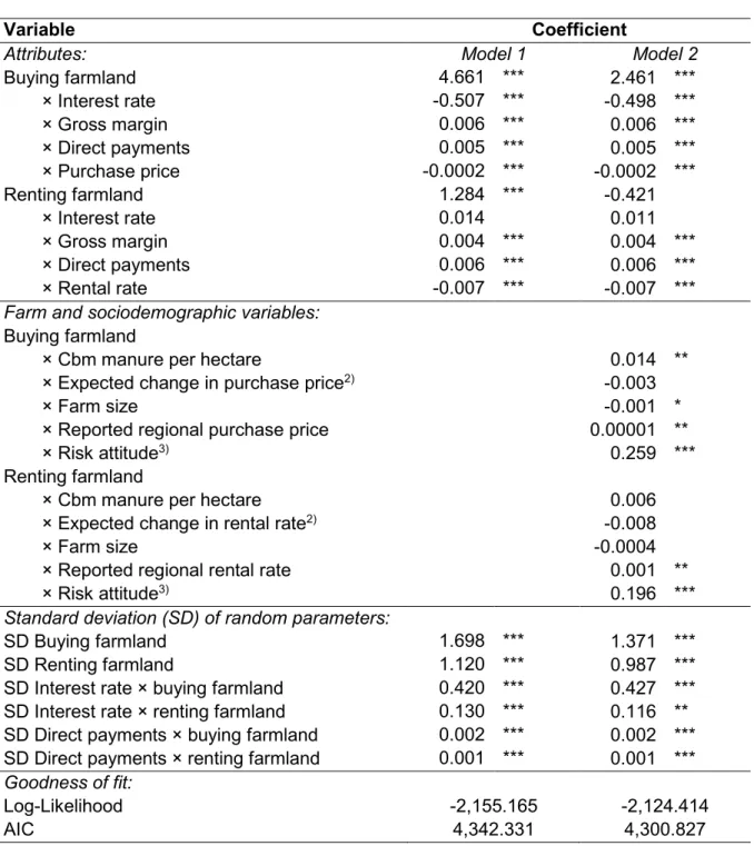
Results from the mixed logit model are presented in Table 4. Model 1 only includes the attributes of the alternatives ‘buying’ and ‘renting farmland’ which were presented to farmers in the DCE. In doing so, Model 1 illustrates how the ‘average farmer’ values the given attributes of the decision to buy or to rent farmland. On average, farmers prefer to buy rather than rent farmland with coefficients for the alternatives ‘buying farmland’ and ‘renting farmland’ of 4.661 and 1.284, respectively. We find a statistically significant negative effect for the attribute

‘interest rate’ on farmers’ decisions to buy farmland. The attributes ‘gross margin’ and ‘direct payments’ have a statistically significant effect on both buying and renting decisions in the DCE. According to a Wald-Test, ‘gross margin’ has a significantly larger effect on the farmers’

decisions to buy than to rent farmland. This is not the case for ‘direct payments’.

Table 4. Results of the Mixed Logit Model (N = 3,060)¹⁾.

Variable Coefficient

Attributes: Model 1 Model 2

Buying farmland 4.661 *** 2.461 ***

× Interest rate -0.507 *** -0.498 ***

× Gross margin 0.006 *** 0.006 ***

× Direct payments 0.005 *** 0.005 ***

× Purchase price -0.0002 *** -0.0002 ***

Renting farmland 1.284 *** -0.421

× Interest rate 0.014 0.011

× Gross margin 0.004 *** 0.004 ***

× Direct payments 0.006 *** 0.006 ***

× Rental rate -0.007 *** -0.007 ***

Farm and sociodemographic variables:

Buying farmland

× Cbm manure per hectare 0.014 **

× Expected change in purchase price²⁾ -0.003

× Farm size -0.001 *

× Reported regional purchase price 0.00001 **

× Risk attitude³⁾ 0.259 ***

Renting farmland

× Cbm manure per hectare 0.006

× Expected change in rental rate²⁾ -0.008

× Farm size -0.0004

× Reported regional rental rate 0.001 **

× Risk attitude³⁾ 0.196 ***

Standard deviation (SD) of random parameters:

SD Buying farmland 1.698 *** 1.371 ***

SD Renting farmland 1.120 *** 0.987 ***

SD Interest rate × buying farmland 0.420 *** 0.427 ***

SD Interest rate × renting farmland 0.130 *** 0.116 **

SD Direct payments × buying farmland 0.002 *** 0.002 ***

SD Direct payments × renting farmland 0.001 *** 0.001 ***

Goodness of fit:

Log-Likelihood -2,155.165 -2,124.414

AIC 4,342.331 4,300.827

1) ***p < 0.01; **p < 0.05; *p < 0.10; Number of random Halton draws = 2,000; AIC = Akaike’s Information Criterion.

2) Individually expected purchase/rental rate change in the next ten years

3) Self-assessed risk attitude on a scale from 0 = ‘not at all willing to take risk’ to 10 = “very willing to take risk.”

Source: Author’s own calculation.

Significant standard deviations in Model 1 reveal heterogeneity around the mean for all variables except gross margin. Hence, we include additional covariates from the farm survey in Model 2 which have the potential to explain the detected heterogeneity by means of interaction terms with the random coefficients. There is no statistically significant effect of the expected change of purchase prices and rental rates in the next ten years on farmers’ decisions

to buy or to rent farmland. Moreover, farmers utility for buying and renting farm land increases with risk aversion. Farmers’ reported regional purchase prices and rental rates for farmland have a statistically significant effect on the alternatives ‘buying’ and ‘renting farmland’ in the DCE. While farm size is negatively related to the alternative ‘buying farmland’, we find a positive effect for the available amount of manure. Both effects are statistically significant.

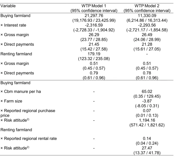
Based on the results in Table 4, we calculate the WTP from all statistically significant coefficients in Model 1 and Model 2.

Table 5. Willingness to pay (WTP) estimates of significant variables (N = 3,060)¹⁾.

Variable WTPModel 1

(95% confidence interval) WTPModel 2 (95% confidence interval)

Buying farmland 21,297.76

(19,176.93 / 23,425.99) 11,330.09 (6,214.86 / 16,313.44)

× Interest rate -2,316.59

(-2,728.33 / -1,904.92) -2,293.56 (-2,721.17 / -1,854.58)

× Gross margin 26.29

(23.77 / 28.85) 26.49

(24.06 / 28.99)

× Direct payments 21.45

(15.42 / 27.58) 21.28

(15.61 / 27.05)

Renting farmland 179.19

(123.32 / 235.08) -

× Gross margin 0.51

(0.45 / 0.57) 0.51

(0.45 / 0.57)

× Direct payments 0.79

(0.61 / 0.96) 0.78

(0.61 / 0.96) Buying farmland

× Cbm manure per ha - 65.02

(0.35 / 129.45)

× Farm size - -3.87

(-8.05 / 0.31)

× Reported regional purchase

price - 0.07

(0.01 / 0.13)

× Risk attitude²⁾ - 1,194.16

(571.42 / 1,821.62) Renting farmland

× Reported regional rental rate - 0.14

(0.04 / 0.24)

× Risk attitude²⁾ - 27.47

(13.37 / 41.78) 1) Krinsky method with 10,000 replications.

2) Self-assessed risk attitude on a scale from 0 = ‘not at all willing to take risk’ to 10 = ‘very willing to take risk.’

Source: Author’s own calculation.

WTP estimates and corresponding confidence intervals are reported in Table 5. Generally, WTP estimates coincide with coefficients presented earlier (Table 4). Considering the constants for Model 1 in Table 5 first, the WTP for the average farmer for the alternatives

an increase in the interest rate by one percent point, the WTP for the alternative ‘buying farmland’ decreases by 2,316.59 €/ha. Bear in mind, that there is no statistically significant effect for ‘interest rate’ on the decision to rent farmland. Moreover, the magnitude of the realised gross margin affects the WTP for the alternatives ‘buying’ and ‘renting farmland’. For an increase of the gross margin by one Euro, WTP estimates for the alternatives ‘buying’ and

‘renting farmland’ rise by 26.29 €/ha and 0.51 €/ha, respectively. Likewise, an additional Euro of direct payments implies an increase of WTP estimates for ‘buying’ and ‘renting farmland’ by 21.45 €/ha and 0.79 €/ha.

Results from Model 2 in Table 5 also reveal the effects for the considered covariates from the farm survey on WTP estimates. It becomes apparent that less risk averse farmers have a higher WTP for both alternatives in the DCE. For every unit increase on the scale of the self- assessed risk attitude, the WTP estimates for ‘buying’ and ‘renting farmland’ of an average farmer increase by 1,194.16 €/ha and 27.47 €/ha, respectively. The magnitude of the reported regional purchase prices and rental rates for farmland only slightly affects farmers’ WTP for

‘buying’ and ‘renting farmland’. Moreover, results from our sample of farmers indicate that the WTP for the alternative ‘buying farmland’ decreases by 3.87 €/ha for every hectare of farm size. Finally, our results reveal that the amount of manure available per hectare of farmland affects the WTP for buying farmland. Farmers’ WTP for ‘buying farmland’ increases by 65.02

€/ha for every additional cbm manure available per hectare. Note, we do not find a comparable effect for the alternative ‘renting farmland’.

4.3 Results from the present value model (normative benchmark)

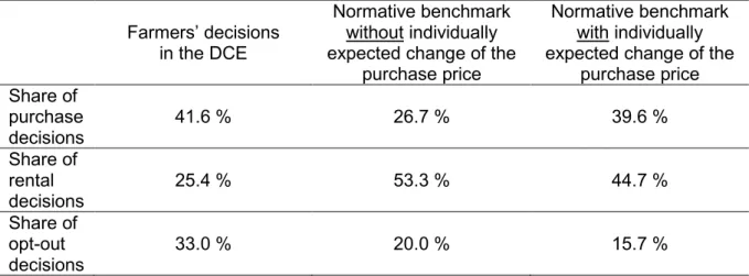
Table 6 contrasts the distribution of farmers’ decisions in the DCE with those from a pure profit- maximizing decision maker (normative benchmark). Farmers chose the alternatives ‘buying farmland’, ‘renting farmland’ and ‘opt out’ in 41.6 %, 25.4 % and 33.0 % of all 3,060 cases (204 farmers ∙ 15 choice sets). In line with results from the mixed logit model, we see that farmers tend to prefer the alternative ‘buying farmland’ in most cases. Present values for the profit- maximizing choices are calculated with and without the individually expected change of farmland prices for a time horizon of the considered ten years as reported by farmers. Bear in mind that farmers expect farmland prices to rise by 12.6 % in the next ten years, on average.

As the growth rate for farmland prices increases the residual value, the alternative ‘buying farmland’ becomes more beneficial if we take farmers’ individual price expectations into account¹. Contrary to farmers’ decisions, the alternative ‘renting farmland’ would be optimal in 53.3 % without individual price expectations and in 44.7 % with individual price expectations of all cases for a profit-maximizing decision maker.

Unlike in the normative benchmark without individual price expectations, farmers chose the alternative ‘buying farmland’ more often. The unexpected low share of the alternative ‘renting farmland’ might indicate that farmers perceive the monetary benefit from managing the additional land as too small and opt-out instead.

1 This does not hold for the alternative ‘renting farmland’. In this case, the expected rise of rental rates of 11.57 % in the next ten years does not affect the present value of the normative benchmark.

Following the experimental design, we assume that the rental contract has a duration of 10 years after which rental rates will be re-negotiated according to future conditions without strategic advantage.

Table 6. Distribution of farmers’ decisions and profit-maximizing choices in the DCE.

(N=3,060).

Farmers’ decisions in the DCE

Normative benchmark without individually expected change of the

purchase price

Normative benchmark with individually expected change of the

purchase price Share of

purchase

decisions 41.6 % 26.7 % 39.6 %

Share of rental

decisions 25.4 % 53.3 % 44.7 %

Share of opt-out

decisions 33.0 % 20.0 % 15.7 %

Source: Author’s own calculation.

Table 7 provides a more detailed analysis of the apparent discrepancy between farmers’ and profit-maximizing decisions in the DCE. Overall, farmers’ decisions only coincide in 45.5 % (48.5 %) of all cases with those of a profit-maximizing decision maker with and without considered price expectations. Differences in terms of the ‘hit rate’ of the benchmark with and without considered individual price expectations tend to be small in general. With a share of 35.2 % (38.0 %), we find the lowest number of matches when the alternative ‘renting farmland’

was optimal in the DCE. In these cases, farmers predominantly preferred to buy the offered land. 54.8 % (54.4 %) of the farmers’ decisions are in line with the normative benchmark when

‘buying farmland’ was the optimal choice while ‘renting farmland’ was the least preferred alternative in these cases. Moreover, farmers act according to the benchmark in 60.5 % (63.3

%) of all cases in which the alternative ‘opt-out’ would generate the maximum present value.

Table 7. Consistency of farmers’ and profit-maximizing decisions in the DCE (N=3,060).

Without individually expected change of the purchase price

With individually expected change of

the purchase price

Decisions according to benchmark 45.5 % 48.5 %

If buying land is optimal according to benchmark…

participants buy land participants rent land participants choose opt-out

54.8 % 9.6 % 35.7 %

54.4 % 14.1 % 31.5 % If renting land is optimal according to

benchmark…

participants buy land participants rent land participants choose opt-out

43.3 % 35.2 % 21.4 %

38.2 % 38.0 % 23.8 % If opting-out of land is optimal according to

benchmark…

participants buy land participants rent land

participants choose opt-out

19.3 % 20.3 % 60.5 %

18.8 % 17.9 % 63.3 %

5

Despite a large body of empirical research dealing with agricultural land markets, there is no consensus on whether developments of purchase prices and rental rates for farmland can be explained or predicted via normative theory. With this in mind, the main objective of this study was to develop a first DCE which is capable of explaining farmers’ individual buying and renting decisions for the same plot of farmland. In each choice decision, a sample of German farmers could buy farmland, rent farmland or chose to opt-out. Hence, we are able to analyse whether farmers in the DCE prefer to buy or rent the offered parcels of farmland. By means of a mixed logit model, we analysed how the attributes ‘gross margin generated’, ‘interest rate’ and

‘magnitude of direct payments’ drive the WTP for farmland prices and rental rates. We included sociodemographic and farm characteristics as well as farmers’ individual price expectations as additional covariates in the model. This information is usually lacking in official reports on farmland prices and rental rates. Moreover, we compared farmers’ choice decisions to those of a pure profit-maximizing decision maker in line with the PVM.

Generally, results from the DCE show that farmers tend to prefer the alternative ‘buying’ over

‘renting farmland’. While the attribute ‘gross margin’ affects both ‘buying’ and ‘renting farmland’, the attribute ‘interest rate’ only affects farmers’ decisions to buy farmland. Moreover, our results indicate that the attribute ‘direct payment’ substantially increases farmers WTP for buying and renting farmland in the experiment. WTP estimates for ‘buying’ and ‘renting farmland’ increase by 21.45 €/ha and 0.79 €/ha for every additional Euro of direct payments transferred to farmers.

This finding might have far reaching policy implications. The income-supporting effect of direct payments is subject to criticism and has been widely discussed in recent years (Guastella et al., 2018). Our findings generally support previous studies which question the effectiveness of direct payments as an income support mechanism. However, it appears that previous studies underestimate the degree to which direct payments are eventually passed through to landowners in the form of increased purchase prices and rental rates for farmland (Allen Klaiber, Salhofer and Thompson, 2017; Breustedt and Habermann, 2011; Graubner, 2018; Ifft, Kuethe and Morehart, 2015; Kirwan and Roberts, 2016).

Moreover, there is heterogeneity in terms of the WTP for the attributes ‘buying’ and ‘renting farmland’ within our sample of German farmers. In this regard, the considered covariates from the farm survey such as farmers’ risk attitude and self-reported regional purchase prices / rental rates affect WTP estimates for buying and renting farmland. Along these lines, farmers’

decisions in the DCE deviate substantially from the normative predictions of the PVM.

Regardless of whether individually expected changes of future purchase prices and rental rates for farmland are considered or not, farmers’ decisions only match optimal decisions following profit-maximization in 45.5 % (48.5 %) of all cases. To date, the PVM is still the standard tool to model farmland values. However, our experimental results indicate that the PVM is not able to explain the complex nature of farmers’ decisions to buy or rent farmland.

Following Clark, Fulton and Scott (1993), a re-thinking of the way in which farmland prices and rental rates are modelled might be necessary.

By design, the external validity of economic experiments, such as the DCE in this study, has limitations (Roe and Just, 2009). Although our results are based on the decisions of real farmers, a generalisation of the results derived from our sample should only be made with

caution. Nevertheless, implications from this study are valuable and pave the way for future research. We contrast farmers’ decisions in the DCE with normative predictions from the PVM.

Future research should elaborate the discrepancy between the experimental and normative results in more detail and quantify the monetary consequences of farmers’ non-optimal decisions in the DCE. In this regard, the consideration of additional covariates might be useful.

Economic experiments have the potential to improve the understanding of farmers’ buying or renting decisions. In this regard, WTP estimates can help to explain the development of farmland prices and rental rates. Finally, our study demonstrates that economic experiments are also well-suited to analyse the impacts of changing agricultural policies on land markets.

To do so, the DCE in our study could be extended in several ways.

6

Allen Klaiber, H., Salhofer, K. and Thompson, S. R. (2017). Capitalisation of the SPS into Agricultural Land Rental Prices under Harmonisation of Payments. Journal of

Agricultural Economics 68(3): 710–726.

Bocquého, G., Jacquet, F. and Reynaud, A. (2013). Expected utility or prospect theory maximisers? Assessing farmers' risk behaviour from field-experiment data. European Review of Agricultural Economics 41(1): 135–172.

Borchers, A., Ifft, J. and Kuethe, T. (2014). Linking the Price of Agricultural Land to Use Values and Amenities. American Journal of Agricultural Economics 96(5): 1307–1320.

Boxall, P. C. and Adamowicz, W. L. (2002). Understanding heterogeneous preferences in random utility models: A latent class approach. Environmental and Resource Economics 23(4): 421–446.

Breustedt, G. and Habermann, H. (2011). The Incidence of EU Per-Hectare Payments on Farmland Rental Rates: A Spatial Econometric Analysis of German Farm-Level Data.

Journal of Agricultural Economics 62(1): 225–243.

Bundesministerium für Ernährung und Landwirtschaft (2017). Daten und Fakten Land-, Forst- und Ernährungswirtschaft mit Fischerei und Wein- und Gartenbau.

Clark, J. S., Fulton, M. and Scott, J. T. (1993). The Inconsistency of Land Values, Land Rents, and Capitalization Formulas. American Journal of Agricultural Economics 75(1):

147.

Croonenbroeck, C., Odening, M. and Hüttel, S. (2019). Farmland values and bidder

behaviour in first-price land auctions. European Review of Agricultural Economics 70(6):

2107.

Das, C., Anderson, C. M. and Swallow, S. K. (2009). Estimating Distributions of Willingness to Pay for Heterogeneous Populations. Southern Economic Journal 75(3): 593–610.

Dessart, F. J., Barreiro-Hurlé, J. and van Bavel, R. (2019). Behavioural factors affecting the adoption of sustainable farming practices: A policy-oriented review. European Review of Agricultural Economics 46(3): 417–471.

Dohmen, T., Falk, A., Huffman, D., Sunde, U., Schupp, J. and Wagner, G. G. (2011).

Individual risk attitudes: Measurement, determinants, and behavioral consequences.

Journal of the European Economic Association 9(3): 522–550.

Duke, J. M. and Gao, T. (2018). An Experimental Economics Investigation of the Land Value Tax: Efficiency, Acceptability, and Positional Goods. Land Economics 94(4): 475–495.

Granello, D. H. and Wheaton, J. E. (2004). Online Data Collection: Strategies for Research.

Journal of Counseling & Development 82(4): 387–393.

Graubner, M. (2018). Lost in space? The effect of direct payments on land rental prices.

European Review of Agricultural Economics 45(2): 143–171.

Guastella, G., Moro, D., Sckokai, P. and Veneziani, M. (2018). The Capitalisation of CAP Payments into Land Rental Prices: A Panel Sample Selection Approach. Journal of

Gutierrez, L., Westerlund, J. and Erickson, K. (2007). Farmland prices, structural breaks and panel data. European Review of Agricultural Economics 34(2): 161–179.

Hanley, N., Ryan, M. and Wright, R. (2003). Estimating the monetary value of health care:

Lessons from environmental economics. Health economics 12(1): 3–16.

Hanson, S. D. and Myers, R. J. (1995). Testing for a time-varying risk premium in the returns to U.S. farmland. Journal of Empirical Finance 2(3): 265–276.

Hennig, S. and Latacz-Lohmann, U. (2016). The incidence of biogas feed-in tariffs on farmland rental rates – evidence from northern Germany. European Review of Agricultural Economics 13(2): 221.

Hensher, D. A., Rose, J. M. and Greene, W. H. (2015). Applied choice analysis. Cambridge:

Cambridge University Press.

Hole, A. R. (2007). A comparison of approaches to estimating confidence intervals for willingness to pay measures. Health economics 16(8): 827–840.

Hu, W., Batte, M. T., Woods, T. and Ernst, S. (2012). Consumer preferences for local production and other value-added label claims for a processed food product. European Review of Agricultural Economics 39(3): 489–510.

Hüttel, S., Odening, M., Kataria, K. and Balmann, A. (2013). Price formation on land market auctions in East Germany: An empirical analysis = Auktionspreise auf dem

ostdeutschen Bodenmarkt. German journal of agricultural economics : GJAE 62(2): 99–

115.

Ifft, J., Kuethe, T. and Morehart, M. (2015). The impact of decoupled payments on U.S.

cropland values. Agricultural Economics 46(5): 643–652.

Kirwan, B. E. and Roberts, M. J. (2016). Who Really Benefits from Agricultural Subsidies?

Evidence from Field-level Data. American Journal of Agricultural Economics 98(4):

1095–1113.

Lancsar, E., Fiebig, D. G. and Hole, A. R. (2017). Discrete Choice Experiments: A Guide to Model Specification, Estimation and Software. PharmacoEconomics 35(7): 697–716.

Lehn, F. and Bahrs, E. (2018). Analysis of factors influencing standard farmland values with regard to stronger interventions in the German farmland market. Land Use Policy 73:

138–146.

List, J. A., Sinha, P. and Taylor, M. H. (2006). Using Choice Experiments to Value Non- Market Goods and Services: Evidence from Field Experiments. Advances in Economic Analysis & Policy 5(2).

Louviere, J. J., Hensher, D. A., Swait, J. and Adamowicz, W. L. (2000). Stated choice methods: Analysis and application. Cambridge: Cambridge Univ. Press.

Luce, R. D. (1959). Individual choice behavior: A theoretical analysis. New York: Wiley.

März, A., Klein, N., Kneib, T. and Musshoff, O. (2016). Analysing farmland rental rates using Bayesian geoadditive quantile regression. European Review of Agricultural Economics 43(4): 663–698.

McFadden, D. (1974). Conditional logit analysis of qualitative choice behavior. In Frontiers in econometrics. New York [u.a.]: Academic Press, 105–142.

Michalek, J., Ciaian, P. and Kancs, d. (2014). Capitalization of the Single Payment Scheme into Land Value: Generalized Propensity Score Evidence from the European Union.

Land Economics 90(2): 260–289.

Nickerson, C. J. and Zhang, W. (2014). Modeling the Determinants of Farmland Values in the United States. In J. M. Duke and J. Wu (eds), The Oxford Handbook of Land Economics. Oxford: Oxford University Press.

Pufahl, A. and Weiss, C. R. (2009). Evaluating the effects of farm programmes: Results from propensity score matching. European Review of Agricultural Economics 36(1): 79–101.

Robison, L. J., Lins, D. A. and VenKataraman, R. (1985). Cash Rents and Land Values in U.S. Agriculture. American Journal of Agricultural Economics 67(4): 794.

Roe, B. E. and Just, D. R. (2009). Internal and external validity in economics research:

Tradeoffs between experiments, field experiments, natural experiments, and field data.

American Journal of Agricultural Economics 91(5): 1266–1271.

Rose, J. M. and Bliemer, M. C. J. (2009). Constructing Efficient Stated Choice Experimental Designs. Transport Reviews 29(5): 587–617.

Schulz, N., Breustedt, G. and Latacz-Lohmann, U. (2014). Assessing Farmers' Willingness to Accept “Greening”: Insights from a Discrete Choice Experiment in Germany. Journal of Agricultural Economics 65(1): 26–48.

Train, K. (2009). Discrete choice methods with simulation. Cambridge: Cambridge University Press.

7

Welcome to our survey about the agricultural land market!

Dear participants,

We would like to welcome you to our study on the topic of the agricultural land market, we are thrilled that you have decided to participate. This study is intended for farmers and is comprised of a participant survey and choice experiment.

The goal of this study is to gain insights into the decision-making behaviour of agricultural producers derived from your choices made in the experiment. Naturally, we also hope that you enjoy participating in our study. The study will take around 20 minutes of your time.

Upon completion of the survey, each participant who has answered all questions carefully and completely will receive an Amazon gift card worth 10€ sent to their email inbox. In addition, five participants of the study will be selected at random to receive a prize of 100€.

In order to avoid technical difficulties, please do not use the back-button of your internet browser, as this will lead to your ejection from the questionnaire and the loss of your entries/answers.

In the case of questions or concerns related to this study, please contact:

Dr. Michael Danne

Georg-August Universität Göttingen

Department of Agricultural Economics and Rural Development Platz der Göttinger Sieben 5

Tel.: 0551-39-4439

E-Mail: michael.danne@agr.uni-goettingen.de

By clicking “Let’s Go” below, you thereby declare your voluntary participation in our survey and your acceptance of the privacy statement.

Dear Participants, to start the survey we would please ask you to provide us some information concerning your farm business.

--- Farm survey ---

--- Here the discrete choice experiment starts --- Dear participants,

in the following experiment, we are interested in learning about your decision-making behaviour with regards to either the purchase or rental of agricultural land. You will be presented with 15 choice sets. Please keep in mind that land offered in each choice set is suitable for agricultural purposes. For each choice set you may decide to either buy or rent the land offered. However, if the conditions pertaining to the utilisation of the land are not acceptable to you, you may also decline to rent/buy the land offered (opt-out).

Now we would like to present to you the framework conditions which are relevant for the decision to rent/buy. Please be aware that the following values may vary from what you may encounter on the real agricultural land market. Please make your decisions as if they pertained to your actual farm business.

• Price: The regional purchase price per hectare (ha) of farmland varies between 10,000 and 50,000 euro. Possible rental rates lie between 200 and 1,000 €/ha. Payment claims shall be made at the time of purchase/rental. In the case of a rental contract, no purchasing option shall be fixed following the end of the contract period.

• Interest Rate: In the case of a land purchase decision, you may borrow up to 100% of the associated costs. The interest rate offered by the bank varies between 1%, 3%, 5% and

• 7%. Gross Margin: With the land that is offered to you, you can achieve a gross margin between 200 and 1,000 €/ha, depending on your production decisions. The gross margin consists of the net sales after direct costs from production are taken into account, such as costs for seed, fertiliser, labour and machinery. The field size and distance to the home are thereby already reflected in the gross margin. Direct payments are not included here.

• Direct Payments: For the purposes of this experiment, please imagine that direct payments will either stay the same or will be reduced over the next 10 years. This reduction affects the area payments (basic and ‘greening’ payments) in the first column of the EU Agricultural Policy. Programme payments, including special bonuses, included in the second column of the EU Agricultural Policy are not altered. The amount of the direct payments that you will receive varies between 0€, 90€, 180€ and 270€.

As you consider each individual choice set, you may refer back to the information regarding the framework conditions at any time. To do so, simply move the mouse symbol on the screen over the question mark symbol in each choice set table.

There are no “correct or “incorrect” answers when it comes to your decision making. Please make you decision as if you were to actually rent or buy the offered land in real life.

--- Here we provided control questions ---

--- Example of Choice Set ---

Please choose your preferred alternative! Please decide whether you would like to rent or buy the offered agricultural land under the given conditions. If you would prefer to neither buy nor rent the land under the given conditions, then please select the option “opt-out.”

Buy Rent Opt-Out Price

The regional purchase prices and rental rates vary between he choice sets. Payment claims shall be made at the time of

purchase/rental. In the case of a rental contract, no purchasing option shall be fixed following the end of the

contract period.

20.000 €/ha 400 €/ha

Interest Rate

In the case of a land purchase decision, you may borrow up to 100% of the associated costs. The interest rate here epresents the interest rate offered by the bank for this given

purchase decision.

7 % 7 %

Gross Margin

You can achieve various gross margins on the offered land dependent on your production decisions and weather conditions. The gross margin consists of the net sales after

direct costs from production are taken into consideration, such as for seed, fertiliser, labour and machinery. The field size and distance to the home are thereby already reflected

in the presented gross margin. Direct payments are not included here.

200 €/ha 200 €/ha

Future Amount of Direct Payments

* For the purposes of this experiment, please imagine that direct payments will either stay the same or could be reduced over the next 10 years. This reduction affects the area payments (basic and ‘greening’ payments) in the first olumn of the EU Agricultural Policy. Programme payments, ncluding special bonuses, included in the second column of

the EU Agricultural Policy are not altered.

0 €/ha 0 €/ha

Which Alternative Do You Choose?

*Additional Information presented in a pop-up window

How important were the following criteria for your decision-making in each of the choice sets?

Unimportant Less Important Important Very Important Direct Payments

Interest Rate Purchase Price Rental Rate Gross Margin Option to Opt-Out

The survey is almost finished!

Next we would like to ask you to provide some statements and perceptions regarding the agricultural land market.

--- Survey on individual expectations about the land market ---

Almost finished!

Lastly, we would like to ask you to provide some personal information!

--- Survey on sociodemographic characteristics ---

The survey is now finished!

Thank you for your participation!