Gravity field processing

Deutsche Geodätische Kommission der Bayerischen Akademie der Wissenschaften

Reihe C Dissertationen Heft Nr. 770

Ilias Daras

Gravity field processing

towards future LL-SST satellite missions

München 2016

Verlag der Bayerischen Akademie der Wissenschaften in Kommission beim Verlag C. H. Beck

ISSN 0065-5325 ISBN 978-3-7696-5182-9

Deutsche Geodätische Kommission der Bayerischen Akademie der Wissenschaften

Reihe C Dissertationen Heft Nr. 770

Gravity field processing

towards future LL-SST satellite missions

Vollständiger Abdruck

der von der Ingenieurfakultät Bau Geo Umwelt der Technischen Universität München zur Erlangung des akademischen Grades eines

Doktor-Ingenieurs (Dr.-Ing.) genehmigten Dissertation

von

Ilias Daras

München 2016

Verlag der Bayerischen Akademie der Wissenschaften in Kommission beim Verlag C. H. Beck

ISSN 0065-5325 ISBN 978-3-7696-5182-9

Deutsche Geodätische Kommission

Alfons-Goppel-Straße 11 ! D – 80 539 München

Telefon +49 – 89 – 23 031 1113 ! Telefax +49 – 89 – 23 031 - 1283 / - 1100 e-mail hornik@dgfi.badw.de ! http://www.dgk.badw.de

Prüfungskommission

Vorsitzender: Univ.-Prof. Dr.-Ing. habil. T. Wunderlich Prüfer der Dissertation: 1. Univ.-Prof. Dr.techn. R. Pail

2. Univ.-Prof. Dr.-Ing. Dr. h.c. mult. R. Rummel (i.R.) 3. Ass. Prof. Dr.-ir. P.N.A.M. Visser,

Technische Universität Delft, Niederlande

Die Dissertation wurde am 29.10.2015 bei der Technischen Universität München eingereicht und durch die Ingenieurfakultät Bau Geo Umwelt am 29.01.2016 angenommen.

.

Diese Dissertation ist auf dem Server der Deutschen Geodätischen Kommission unter <http://dgk.badw.de/>

sowie auf dem Server der Technischen Universität München unter elektronisch publiziert

Diese Dissertation ist auf dem Server der Deutschen Geodätischen Kommission unter <http://dgk.badw.de/>

sowie auf dem Server der Technischen Universität München unter

<###################################> elektronisch publiziert © 2016 Deutsche Geodätische Kommission, München

Alle Rechte vorbehalten. Ohne Genehmigung der Herausgeber ist es auch nicht gestattet,

die Veröffentlichung oder Teile daraus auf photomechanischem Wege (Photokopie, Mikrokopie) zu vervielfältigen.

ISSN 0065-5325 ISBN 978-3-7696-5182-9

Summary

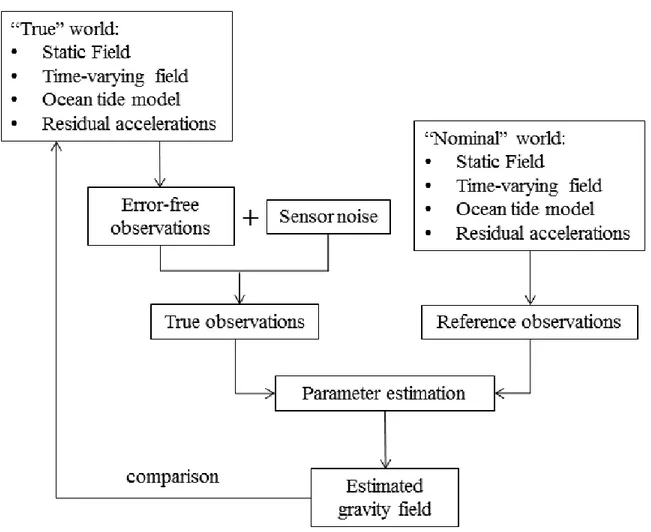
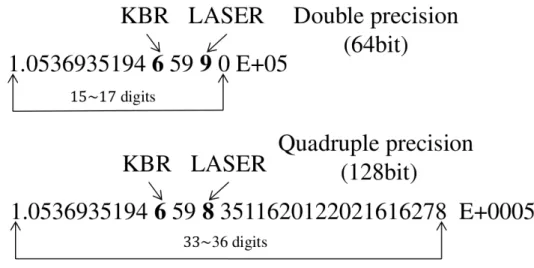
This study focuses on important aspects concerning gravity field processing of future Low-Low Satellite- to-Satellite Tracking (LL-SST) satellite missions. Closed-loop simulations taking into account error models of new generation instrument technology are used to estimate the gravity field accuracy that future missions could provide. Limiting factors are identified, and methods for their treatment are de- veloped. The contribution of all error sources to the error budget is analyzed. It is shown that gravity field processing with double precision may be a limiting factor for exploiting the nm-level accuracy of a laser interferometer. An enhanced numerical precision processing scheme is proposed instead, where double and quadruple precision is used in different parts of the processing chain. It is demonstrated that processing with enhanced precision can efficiently handle laser measurements and take full advantage of their accuracy, while keeping the computational times within reasonable levels. However, error sources of considerably larger impact are expected to affect future missions, with the accelerometer instrument noise and temporal aliasing effects being the most significant ones. The effect of time-correlated noise such as the one present in accelerometer measurements, can be efficiently handled by frequency de- pendent data weighting. Residual time series that contain the effect of system errors and propagated accelerometer and laser noise, is considered as a noise realization with stationary stochastic properties.

The weight matrix is constructed from the auto-correlation functions of these residuals. Applying the

weight matrix to a noise case considering all error sources leads to reduction of the error level over the

complete spectral bandwidth. Co-estimation of empirical accelerations does not show the same efficiency

in reducing the propagated noise with the applied processing strategy. Temporal aliasing effects are re-

duced essentially by adding a second pair of satellites at an inclined orbit. Compared to a GRACE-type

near-polar pair, such a Bender-type constellation delivers solutions with major improvements in terms of

de-aliasing potential and recovery performance. When the integrated effect of all geophysical processes

is recovered, the maximum spatial resolution of 11-day solutions can be increased from 715 to 315 km

half-wavelength. A further reduction of temporal aliasing errors is possible by co-parameterizing low

resolution gravity fields at short time intervals, together with the higher resolution gravity field which is

sampled at a longer time interval. One day was found to be the optimal sampling period for reducing

the error levels in the solutions. A uniform sampling at the co-parameterized short periods, is a prereq-

uisite for an efficient reduction of aliasing errors. High frequency atmospheric signals are captured by

daily solutions to a large extent. Hence co-parameterization at daily basis results in significant reduction

of aliasing caused by their under-sampling. This enables future gravity satellite missions to deliver the

complete spectrum of Earth’s geophysical processes. The corresponding by-products of daily gravity

field solutions are expected to be very useful to atmospheric science and open doors to new fields of

application.

Zusammenfassung

Diese Doktorarbeit befasst sich schwerpunktmäßig mit der Schwerefeldprozessierung zukünftiger Low- Low Satellite-to-Satellite (LL-SST) Satellitenmissionen. Um die Genauigkeit zukünftiger Satellitenmis- sionen abzuschätzen, wurden Closed-loop Simulationen unter Einbeziehung von Fehlermodellen neuer Instrumentengenerationen durchgeführt. Einschränkende Faktoren werden erörtert und entsprechende Lösungansätze entwickelt. Der Beitrag aller Fehlerquellen zum gesamten Fehlerbudget wird quan- tifiziert. Es wird nachgewiesen, dass die Schwerefeldprozessierung mit doppelter Rechengenauigkeit ein limitierender Faktor für die Ausschöpfung der nm-Messgenauigkeit eines Laserinterferometers sein kann. Ein alternatives Prozessierungsschema erhöhter Rechengenauigkeit wird stattdessen vorgeschla- gen, in dem doppelte und vierfache Rechengenauigkeit in verschiedenen Prozessierungsschnritten verwendet wird. Es wird demonstriert, dass in diesem Fall Laserbeobachtungen mittels erhöhter Genauigkeit wirkungsvoll prozessiert werden können und deren Präzision voll ausgenutzt werden kann.

Gleichzeitig bleibt der Rechenaufwand in angemessenen Grenzen. Allderdings, werden sich voraus- sichtlich andere Fehlerquellen stärker auf zukünftige Satellitenmissionen auswirken. Das Rauschen der Beschleunigungsmesser und die Effekte von zeitlichem Aliasing stellen die beiden größten Fehlerquellen dar. Fehler infolge von zeitkorreliertem Rauschen, wie z.B. in den Beobachtungen der Beschleu- nigungsmesser, können wirkungsvoll mittels frequenzabhängiger Datengewichtung behandelt werden.

Eine Zeitreihe von Residuen, die den Effekt vom Systemrauschen, propagiertem Beschleunigungsmess-

rauschen und Laserrauschen beinhaltet, werden als Rauschrealisierung mit stationären stochastischen

Eigenschaften berücksichtigt. Basierend darauf wird die Gewichtungsmatrix durch Autokorrelationfunk-

tionen erstellt. Die Einbeziehung der Gewichtungsmatrix in einem Fall, der alle Fehlerquellen betrachtet,

führt zur Reduzierung des Fehlerniveaus über das gesamte Spektrum. Dagegen führt das Mitschätzen

von empirischen Beschleunigungen nicht zu derselben gleichmässigen Reduzierung von Fehlern. Effekte

von zeitlichem Aliasing reduzieren sich wesentlich durch die Erweiterung um ein zweites Satellitenpaar

mit inklinierter Bahn. Im Vergleich zu einem GRACE-ähnichen Paar mit fast polarer Bahn liefert eine

solche Bender Konstellation verbesserte Ergebnisse hinsichtlich der Reduzierung von Aliasingeffekten

und erzielbarer Genauigkeit. Wenn eine integrierte Wirkung aller geophysikalischer Prozesse betra-

chtet wird, kann sich die maximale räumliche Auflösung einer 11-tägigen Lösung von 715 auf 315

km halbe Wellenlänge steigern. Eine weitere Reduzierung der zeitlichen Aliasing-Effekte ist möglich

durch Mitschätzung von niedrig aufgelösten Schwerfeldlösungen über kurze Zeitspannen, zusammen

mit der hoch aufgelösten Schwerfeldlösung, die über eine längere Zeitspanne abgetastet wird. Der optimale Abtastzeitraum für kurze Zeitspannen zur Reduzierung des Fehlerniveaus beträgt einen Tag.

Ein einheitliches Abtasten innerhalb der kurzer Zeitspannen ist eine Voraussetzung für eine effektive

Reduzierung der Aliasingfehlern. Hochfrequente Signale der Atmosphäre können in großem Maß aus

täglicher Parametrisierung erfasst werden. Somit führt die Co-Parametrisierung in täglichen Zeitspan-

nen zu einer signifikantent Reduzierung der Aliasingfehler. Das ermöglicht zukünftigen Satellitenmis-

sionen, das ganze Spektrum von geophysikalischen Prozessen der Erde zu erfassen. Die entsprechen-

den täglichen Schwerefeldlösungen stellen zusätzliche Produkte dar, die nützlich für die Atmosphären-

forschung sein konnen. Damit öffnen sich Perspektiven für gänzlich neue Anwendungen.

Contents

Contents xi

1 Introduction 1

1.1 Background . . . . 1

1.2 Motivation and objectives of this study . . . . 2

1.3 Outline . . . . 3

2 Earth’s gravity field determination from satellite observations 5 2.1 Perturbing forces acting on a satellite . . . . 5

2.1.1 Earth’s gravitational field . . . . 6

2.1.2 Direct tides (3 ^{r d} Body) . . . . 10

2.1.3 Earth tides . . . . 10

2.1.4 Non-gravitational forces . . . . 11

2.2 Geopotential and its functionals . . . . 12

2.3 Dedicated gravity satellite missions . . . . 15

2.3.1 The CHAMP mission . . . . 16

2.3.2 The GRACE mission . . . . 16

2.3.3 The GOCE mission . . . . 18

2.4 Concepts for future satellite gravity missions . . . . 19

2.4.1 The GRACE Follow-On mission . . . . 20

2.4.2 Next Generation Gravity Missions (NGGMs) . . . . 20

3 Description of the simulation environment for the gravity field recovery 23 3.1 Outline of the simulation environment . . . . 23

3.2 Coordinate and time systems . . . . 25

3.3 Simulation of the satellite orbits . . . . 27

3.4 Functional model . . . . 28

3.5 Formulation of the NEQ system . . . . 30

3.6 Solution of the NEQ system . . . . 35

3.6.1 Parameterization of the unknown parameters . . . . 35

3.6.2 Parameter pre-elimination . . . . 37

3.6.3 Accumulation of the NEQs . . . . 38

4 Design aspects and error budget of future dedicated gravity satellite missions 41 4.1 Orbit design . . . . 41

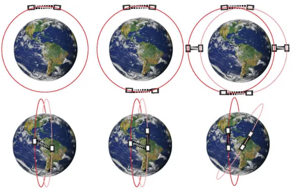
4.2 Satellite formation flights . . . . 43

4.3 Selected orbits for the simulations . . . . 46

4.4 Science and mission requirements . . . . 47

4.5 Noise models for the performance of the instruments . . . . 50

4.5.1 Laser interferometer errors . . . . 50

4.5.2 Accelerometer errors . . . . 50

4.5.3 Star camera errors . . . . 51

4.5.4 Residual drag accelerations . . . . 52

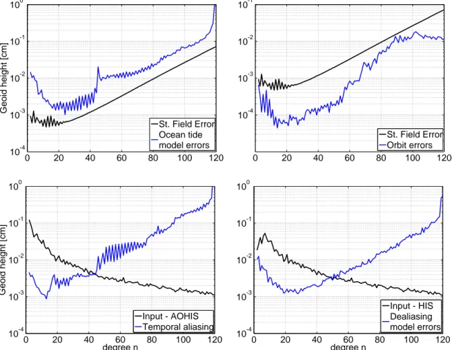
4.6 Error budget analysis . . . . 54

5 Gravity field processing with enhanced numerical precision 61 5.1 Concept of enhanced numerical precision . . . . 61

5.2 Usage of enhanced numerical precision in the gravity field processing chain . . . . 63

5.3 Benefits of processing with enhanced numerical precision . . . . 65

6 Methods of noise reduction 73 6.1 Frequency dependent data weighting . . . . 73

6.2 Empirical parameterization . . . . 76

6.3 Simulation results of processing with noise-reduction methods . . . . 77

7 Treatment of temporal aliasing e ff ects 85 7.1 Temporal aliasing for NGGMs . . . . 85

7.1.1 Benefits of a Bender-type SFF constellation . . . . 85

7.1.2 Processing strategies for retrieval content . . . . 87

7.2 Co-parameterization of low spatial resolution gravity field solutions at higher frequencies 89 7.2.1 Noise-free case analysis . . . . 93

7.2.2 Noise-case analysis . . . . 97

7.2.3 Sequential co-parameterization . . . . 103

7.2.4 Assessment of individual aliasing components . . . . 105

7.2.5 Processing of an alternative constellation . . . . 109

CONTENTS xiii 7.3 Retrieval content of NGGM gravity field solutions . . . . 112

8 Conclusions 117

Acronyms 121

List of Figures 125

List of Tables 131

Bibliography 133

Chapter 1

Introduction

1.1 Background

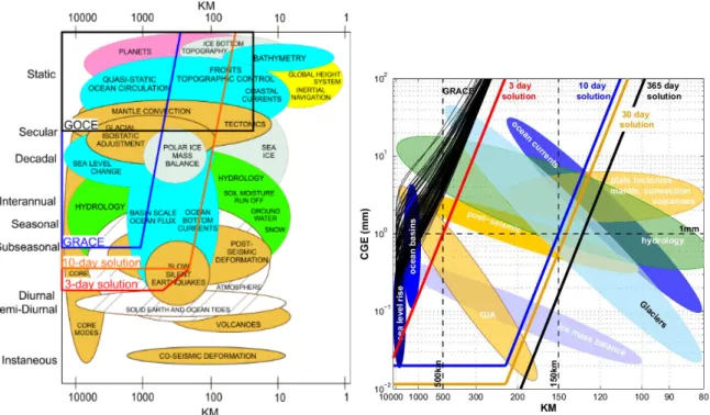
Earth is a living planet that is subject to substantial changes due to processes and interactions between its geophysical sub-systems; namely the atmosphere, hydrosphere, biosphere and geosphere. A significant amount of these processes is related to mass redistribution in the Earth system and thus is translated into changes of the gravity field of the Earth. Knowledge about Earth’s gravity field properties is therefore fundamental for many applications of Earth sciences. Gravity measurements contribute to the computa- tion of geoid models used for regional height reference systems, thus allowing the combination of Global Positioning System (GPS) with classical leveling techniques. Global satellite observations are used for the computation of a global geoid model, with the ambitions to unify regional height systems into a global reference system, hence making local or continental height systems comparable. Geoid models are also very useful in the field of oceanography, where geoid heights are subtracted from sea surface heights (measured by satellite altimetry), to deliver the sea surface topography. The latter is used in ocean circulation modeling, which is the basis for understanding the global heat balance. Knowledge of Earth’s gravity field is therefore implicitly a very valuable input for the computation of global climate models.

Moreover, temporal gravity field changes are used to quantify changes in the global water balance, such as the polar ice cap melting, mean sea level change and seasonal changes in the water balance of large river basins. Global gravity observations contribute to the computation of hydrological, glaciological and Glacial Isostatic Adjustment (GIA) models. Finally, geophysical and geodynamical models used in solid Earth applications are improved from gravity field information. These models are very useful for a better interpretation of seismic events, volcanic processes and plate tectonics, as well as for the exploration of natural resources.

Space observations provide the only means to monitor and assess changes of Earth’s sub-systems on a

global and long-term perspective. They deliver long and continuous time series of important Earth system

parameters, which contribute to the analysis and prediction of these changes. Mass distribution and

transport processes in the Earth system consist mainly of dynamic processes in cryosphere, continental

hydrology, ocean, atmosphere and solid Earth. At the end of the 20th century, tracking data from satellite missions using various observation techniques (e.g. SLR, Doppler, PRARE, Doris or GPS) have been used to improve our knowledge on Earth’s gravity field. In 2000, the era of dedicated geopotential missions began with the launch of the Challenging Minisatellite Payload (CHAMP) (ended in 2010) (Reigber, 1995). The Gravity Recovery and Climate Experiment (GRACE) (2002 ∼ present) (Tapley et al., 2004) and the Gravity field and steady-state Ocean Circulation Explorer (GOCE) (2009 ∼ 2013) (Rummel et al., 2011) dedicated gravity missions that followed, resulted in remarkable improvements in the knowledge of Earth’s time-varying and static gravity field, respectively. The great success of GRACE in mapping Earth’s mass changes, established its products applicable to a large spectrum of Earth sciences. The continuity of the time-varying gravity field time series, is enabled by the upcoming launch (August 2017) of GRACE’s successor, namely the GRACE Follow-On (GRACE-FO) mission (Flechtner et al., 2014a). GRACE-FO is a gap-filling mission that will cover the timespan between GRACE and Next Generation Gravity Missions (NGGMs) to be launched in the mid-term future (after 2020).

1.2 Motivation and objectives of this study

Dedicated gravity missions delivering observations for a period longer than 15 years, have left a pre- cious heritage for studies of future satellite mission designs. The employment of different measuring techniques such as High-Low Satellite-to-Satellite Tracking (HL-SST), LL-SST and gravitational gra- diometry, have been extensively investigated for their ability to improve specific properties of the static and time-varying part of Earth’s gravity field. Analysis of the on-board sensor data led to assessment of their quality and estimation of their contribution to the gravity field error budget. Investigations concern- ing orbit design pointed out physical constraints caused by insufficient sampling. The aforementioned limitations constitute important lessons learnt from the dedicated gravity missions. These lessons, to- gether with the needs and requirements of the scientific community, establish a solid background for mission design of NGGMs.

Main subject of this study is the gravity field processing of future LL-SST satellite missions. New generation instrument technology is expected to deliver measurements of substantially higher accuracy compared to the ones derived from current sensors. Key instrument of LL-SST missions is the inter- satellite ranging unit, which enables the detection of mass changes taking place below the satellites’

orbital altitude. Laser interferometry is planned to substitute the K-Band Ranging (KBR) technology

used so far in GRACE mission for the inter-satellite ranging. This will improve the measuring accuracy

from µm to nm level, and raise potential for big improvements in terms of spatial resolution. However,

this level of accuracy has to be contemplated with the noise levels from other error sources and limita-

tions concerning processing accuracy. So far, gravity field processing accuracy has always been below

the noise levels of observations. Advances in metrology of sensors such as the inter-satellite ranging

instrument, may raise the demands for processing accuracy. In this study, we carefully address these

1.3 Outline 3 questions and propose solutions to the problems encountered.

The quantification of the contribution of all error sources to the error budget is a very important task for designing NGGMs. Comprehending the way each noise source propagates into the error spectrum, plays an important role for their effective treatment. In the frames of this study, we perform assessment of their contribution, and give special attention to the specific bandwidth part of the error spectrum each noise source is influencing. We develop methods for reducing the effect of error sources at the level of gravity field processing. Those methods are then applied for NGGMs of in-line GRACE-type formation, as well as for novel mission designs that constitute a constellation of satellites. It is also investigated, in which way the addition of a second pair of satellites improves the system’s isotropy, and contributes to the reduction of temporal aliasing effects. The latter remains nevertheless one of the biggest contributors to the error budget of NGGMs. When using two pairs of satellites, temporal and spatial resolution are increased. That makes high frequency gravity field information taking place on large scales, easier to be retrieved. A further reduction of temporal aliasing effects is possible, when this information is taken into account and is properly assigned to the averaged solution. This leads to a gravity field approach with a wide spectrum of parameterization possibilities. This approach was implemented and investigated in this study, in the framework of a European Space Agency (ESA)-funded project with the name “Assessment of Satellite Constellations for Monitoring the Variations in Earth Gravity Field - SC4MGV” (Iran Pour et al., 2015). The spectrum of choices is explored and their effect is individually investigated. Possible relations between orbit design choices and the effectiveness of this method are also investigated, and recommendations on optimal parameterization choices are given. Finally, the relative improvements of solutions from such a NGGM compared to the state-of-the-art missions are discussed.

1.3 Outline

Chapter 2 gives the theoretical background for determining Earth’s gravity field from satellite obser-

vations. It also presents the mission details of dedicated gravity satellite missions of the past and the

present, and concludes by discussing concepts for future missions. Chapter 3 gives an overview of the

simulation environment for the gravity field recovery. At first, the coordinate and time systems used are

described. As a next step, the method for orbit simulation and the mathematical description of the func-

tional model are presented. Finally, the formulation and solution of the system are described. Chapter

4 starts with an overview of the orbit designs for present and future gravity satellite missions. A brief

discussion on science and mission requirements for future missions follows. Next, the noise models for

the instrument performance used in the simulations are given, and results of closed-loop simulations for

the error-budget analysis are presented. Chapter 5 reports the limitations when processing with standard

accuracy, and investigates the use of enhanced accuracy in the gravity field processing chain. Chapter 6

presents the investigated methods of noise reduction, and analyzes their effect in gravity field processing

at the presence of all noise sources. Chapter 7 deals with the treatment of temporal aliasing effects for

NGGMs. Finally, Chapter 8 gives the conclusions of this study.

Chapter 2

Earth’s gravity field determination from satellite observations

This chapter is dedicated to the description of the space methods that are used to determine features of the gravity field and the figure of the Earth. At first, the perturbing forces acting on a satellite are reviewed.

As a next step, an overview of the dedicated gravity satellite missions of the past and the present is given.

Finally, the state-of-the-art plans and challenges for NGGMs are presented.

2.1 Perturbing forces acting on a satellite

A near-earth artificial satellite flies around the Earth with an orbit that is slightly perturbed from its ideal Kepler motion. In case of a perturbed motion, the equation of motion takes the form of an inhomogeneous differential equation of second order:

¨r + G M _E

r ³ r = d ¨r, (2.1)

where G is the Newtonian gravitational constant, M _E is the Earth’s total mass and r/r denotes a unit

vector pointing from the center of the Earth to the satellite. For the analytical solution of Eq. (2.1), per-

turbation theory may be applied, where initially the homogeneous part of Eq. (2.1) is considered, leading

to a Keplerian orbit. Each disturbing acceleration d ¨r causes temporal variations in the orbital parameters

that lead to an osculating ellipse which deviates from the Keplerian orbit. Those deviations are caused by

perturbing forces that act on the satellite and are categorized into gravitational (or conservative) and non-

gravitational (or non-conservative) forces. The gravitational forces are by far the strongest and mainly

determine the satellite’s orbit. They are induced by the gravitational attraction of the non-spherical part

of Earth’s gravity field and other celestial bodies (e.g. Sun, Moon and other planets) as well as tides

(ocean, solid Earth, pole and third bodies). Non-gravitational forces include thrust forces, atmospheric

drag, solar radiation pressure and Earth’s reflected radiation (Earth albedo).

2.1.1 Earth’s gravitational field

Newton’s law of gravitation describes the attraction of two points with masses m 1 and m 2 separated by a distance l:

F = G m 1 · m 2

l ² , (2.2)

where G is the Newtonian gravitational constant in Système International d’unités (SI) units:

G = 6.6743 · m ³ kg ^{− 1} s ^{− 2} . (2.3)

The gravitational field can be studied by calling one mass the attracting mass and the other the attracted mass. For simplicity the attracted mass is set equal to unity and the attracting mass is denoted by m. The gravitational force will then be equal to:

F = G m

l ² . (2.4)

In geodesy we are considering the attraction of systems of point masses or of solid bodies. Thus it is easier to deal with a function such as the potential of gravitation, which is related to the force function in vector notation as

F = grad(V ) (2.5)

Assuming that the point masses are distributed continuously over a volume υ with density ρ, the potential can be given by Newton’s integral

V = G

$

υ

ρ

l dυ (2.6)

Outside the attracting masses, the density ρ is zero and the Laplace equation is satisfied:

∆ V = 0 (2.7)

where the symbol ∆ is the so-called Laplacian operator. The solutions of Eq. (2.7) are called harmonic functions. Thus, the gravitational potential outside the Earth is also a harmonic function, whose solution is given by the sum of the surface spherical harmonics Y _n (Hofmann-Wellenhof and Moritz, 2006):

V = X ∞

n=0

Y n (θ , λ)

r ⁿ⁺¹ (2.8)

where r (radius vector), θ (polar distance) and λ (geocentric longitude) represent the spherical coordi- nates. The Laplace’s differential equation for surface spherical harmonics has solutions given by the following functions:

Y _nm ^c (θ , λ) = P nm (cosθ )cosm λ and Y _nm ^s (θ , λ) = P nm (cosθ )sinmλ, (2.9)

2.1 Perturbing forces acting on a satellite 7 where P _nm (cosθ) is the Legendre function. Due to the linearity of those solutions, their combination will also be a solution that delivers the general expression for the surface spherical harmonics Y n :

Y _n (θ , λ) =

n

X

m=0

(a _nm cosm λ + b _nm cosmλ)P _nm (cosθ ) (2.10) where a nm and b nm are arbitrary constants. Substituting Eq. (2.10) to Eq. (2.8), the gravitational potential can be derived as an arbitrary function f (θ , λ) which is expanded into a series of surface spherical harmonics on the surface of the sphere:

f (θ , λ ) = V = X ∞

n=0

Y _n (θ , λ) r ⁿ⁺¹ =

X ∞ n=0

1 r ⁿ⁺¹

n

X

m=0

(a _nm cosmλ + b _nm cosmλ)P _nm (cosθ), (2.11) Earth related applications benefit from the properties of spherical harmonics, when they are represented as an orthogonal set of solutions to the Laplace equation. The orthogonality property allows for a for- ward and inverse transform of a function to its spectrum. This is a reason why gravity field functionals are formulated in terms of spherical harmonic coefficients. Using the orthogonality properties of the functions included in (2.11):

R nm =P _nm (cosθ)cosm λ, (2.12)

S nm =P nm (cosθ)sinmλ,

the equations for the constant coefficients a nm and b nm can be derived:

a n0 = 2n + 1 4π

"

σ

f (θ , λ)P _n (cosθ )dσ;

a nm = 2n + 1 2π

(n − m)!

(n + m)!

"

σ

f (θ , λ) R ^nm (θ , λ)dσ b nm = 2n + 1

2π

(n − m)!

(n + m)!

"

σ

f (θ , λ) S nm (θ , λ)dσ



 

 

 

 



 

 

 

 



(m , 0). (2.13)

In connection with satellite dynamics, Eq. (2.11) is often written in a form where the gravitational potential outside the Earth is expressed (Hofmann-Wellenhof and Moritz, 2006):

V (r, θ , λ) = G M E

r



 



 

 1 +

X ∞ n=1

X n

m=0

R E

r n

[C _nm R ^nm (θ , λ) + S nm S ^nm (θ , λ)]



 



 



, (2.14)

where R _E is the mean equatorial radius of the Earth, so that it satisfies:

C _nm = 1 G M R ⁿ _E A _nm S _nm = 1

G M R ⁿ _E B _nm



 

 

 



 

 

 



(m , 0). (2.15)

The A _nm and B _nm coefficients can be determined from the boundary values of gravity at the Earth’s surface:

A n0 = G

$

earth

r

ⁿ P n (cosθ

)dM ;

A nm = 2 (n − m)!

(n + m)! G

$

earth

r

ⁿ R nm (θ

, λ

)dM B nm = 2 (n − m)!

(n + m)! G

$

earth

r

ⁿ S nm (θ

, λ

)dM



 

 

 

 



 

 

 

 



(m , 0), (2.16)

where (r

, θ

, λ

) are the spherical coordinates of a mass element dM inside Earth and (r, θ , λ) of a point at which the potential is to be determined. The conventional harmonics R nm and S nm can be replaced by other functions which are easier to handle, namely the fully normalized harmonics R nm and S nm given by (Hofmann-Wellenhof and Moritz, 2006):

R ⁿ⁰ (θ , λ) = √

2n + 1 R ⁿ⁰ (θ , λ) ≡ √

2n + 1P _n (cosθ);

R nm (θ , λ) = s

2(2n + 1) (n − m)!

(n + m)! R nm (θ , λ) S nm (θ , λ) =

s

2(2n + 1) (n − m)!

(n + m)! S nm (θ , λ)



 

 

 

 

 

 

 

 

 

 

(m , 0). (2.17)

Similarly the corresponding fully normalized coefficients will be given by:

C n0 = 1

√ 2n + 1 C n0 ;

2.1 Perturbing forces acting on a satellite 9

C _nm =

s (n + m)!

2(2n + 1)(n − m)! C _nm S nm =

s (n + m)!

2(2n + 1)(n − m)! S nm



 

 

 

 

 

 

 

 

 

 

(m , 0). (2.18)

From a geometrical representation point of view, the spherical harmonics can be divided to zonal, tesseral and sectorial harmonics. Zonal are the harmonics with order equal to zero (m = 0), leading to an independence on longitude λ. The harmonics with equal degree and order (m = n) are called sectorial harmonics and do not depend on latitude φ. All other harmonics have m , 0 and m , n, are latitude and longitude dependent and are called tesseral harmonics. Zonal harmonics effect the satellite orbits to a much greater extent than tesseral harmonics, by influencing mostly the secular and long-periodic perturbations of the satellite’s orbital elements a, e, i, e.t.c. Therefore, long observation periods with several satellite revolutions are needed in order to detect their influence in changes of orbital parameters.

On the other hand, the perturbations due to tesseral harmonics lead to much shorter periods.

The very first spherical harmonic coefficients are of particular interest in geodesy. With Eq. (2.16) one can compute the zero-degree term A _nm :

A ₀₀ = G

$

Earth

dM = G M _E , (2.19)

which produces a zero-degree component of the geopotential V 00 being nothing else than the gravitational potential of a point mass equal to the total mass of the Earth. Accordingly, the first-degree coefficients yield:

A 10 = G

$

Earth

z

dM, A 11 = G

$

Earth

x

dM, B 11 = G

$

Earth

y

dM . (2.20) Those three first-degree coefficients will be equal to zero if the origin of the used coordinate system coincides with the geocenter. In that case, the center of mass of the Earth coincides with the center of the Figure of the solid Earth. In general, LEO gravity field satellite missions such as the GRACE mission cannot provide accurate estimates of the geocenter motion since its effect cannot be separated from other parameters. As a result, the first-degree coefficients estimated from their measurements are of no value (Rietbroek et al., 2012).

Introducing the moments of inertia of the Earth with respect to the x − , y − , z − axes J _x =

$

Earth

( y

² + z

² )dM, J _y =

$

Earth

(z

² + x

² )dM, J _z =

$

Earth

(x

² + y

² )dM , (2.21)

and the product of inertia of the Earth, J xy =

$

Earth

x

y

dM, J yz =

$

Earth

y

z

dM , J xz =

$

Earth

z

x

dM, (2.22)

we end up with the degree two coefficients (Hofmann-Wellenhof and Moritz, 2006):

A 20 = G[(J _x + J _y )/2 − J _z ], A 21 = G J _xz , A 22 = 1

4 G( J _y − J _x ) B 21 = G J yz , B 22 = 1

2 G J xy .

(2.23)

If the z axis of the coordinate system coincides with the Earth’s principal axis of moment of inertia, J xz , J yz and consequently A 21 , B 21 will be equal to zero. Coefficient A 20 is the largest perturbation term and is related to the ellipsoidal character of the Earth. It depends on the difference between the mean equatorial moment of inertia and that around the z axis, thus characterizing its flattening. Coefficient A 22

is related to the difference in the moment of inertia with respect to the two axes in the equatorial plane, and thus it describes the equatorial non-symmetry of the mass distribution inside the Earth.

2.1.2 Direct tides (3 ^{r d} Body)

The satellite as well as the Earth itself are affected by gravitational forces of other celestial bodies, mainly the Sun and the Moon. The resulting force acting on the satellite is called direct tidal force. The acceleration of a satellite due to the attraction caused by a 3 ^{r d} body with a point mass M is given by:

¨r = G M s − r

| s − r | ³ − s

| s | ³

!

, (2.24)

where s and r are the geocentric position vectors of the satellite and the celestial body respectively. For a typical Low Earth Orbiter (LEO) gravity satellite where the Sun and the Moon are far much further away from the Earth, the forces exerted from the Sun and the Moon are much smaller than the central attraction of the Earth. Therefore, for many applications the solar and lunar geocentric coordinates are not required to be known at the highest precision. Assuming an unperturbed motion of the Earth around the Sun, low-precision simplified equations for the solar and lunar coordinates are given by Montenbruck and Gill (2000).

2.1.3 Earth tides

Earth tides are a result of the attracting forces exerted by the gravitation of the Sun and the Moon, which lead to a time-varying deformation of the Earth. This deformation has an effect on the motion of the satellites. The Earth tides are categorized in solid Earth, ocean and pole tides, which are briefly discussed in the following section. For a more detailed description we refer to Petit and Luzum (2010).

Solid Earth tides

The Earth’s solid body is elastic to first order. Thus, it responds to lunisolar gravitational attraction with

small periodic deformations which are called solid Earth tides. Similarly to the Earth’s static gravity

field, spherical harmonics can be used to expand the solid Earth tidal-induced gravity potential that affect

2.1 Perturbing forces acting on a satellite 11 the perturbed motion of the satellite. The time-dependent corrections to the unnormalized geopotential coefficients can be computed according to Sanchez (1975):



 



 



∆ C nm

∆ S _nm



 



 



= 4k _n G M G M E

! R _E R

s (n + 2)(n − m)! ³

(n + m)! ³ P _nm (sin φ)



 



 



cos(mλ) sin(mλ)



 



 



(m , 0). (2.25) where M and R represent the mass and the geocentric distance of the Sun or the Moon, φ and λ their corresponding Earth-fixed latitude and longitude and k n the Love numbers of degree n.

Ocean tides

The response of the oceans to the lunisolar gravitational attraction is known as ocean tides. It is another time-variable phenomenon occurring in the ocean and causing cyclic variations in the local sea level.

This oceanic mass redistribution can be represented, as well as the solid Earth tides, by corrections of unnormalized geopotential coefficients (Montenbruck and Gill, 2000):



 



 



∆ C nm

∆ S nm



 



 



= 4πGR ² _E ρ _w G M _E

1 + k

_n 2n + 1



 

 



 

 

 P

s(n,m) (C _snm ⁺ + C _snm ⁻ cos θ _s ) + (S _snm ⁺ + S _snm ⁻ sin θ _s ) P

s(n,m) (S _snm ⁺ + S _snm ⁻ cos θ s ) + (C _snm ⁺ + C _snm ⁻ sin θ s )



 

 



 

 



(m , 0). (2.26)

where ρ w is the density of the seawater, k

_n are the load-deformation coefficients of degree n, C _snm ^± and S _snm ^± are the ocean tide coefficients in meters for the tide constituent s, θ _s is the weighted combination of the six Doodson variables. The Doodson variables are closely related to the arguments of the nutation series and principally denote the fundamental arguments of the Sun and Moon orbits.

Pole tides

Pole tides are caused by the contribution of the polar motion to the centrifugal potential due to Earth rotation. They affect mainly the geopotential coefficients C 21 and S 21 and can cause up to 25 mm tidal response in radial direction and 7 mm in horizontal direction (Petit and Luzum, 2010)

2.1.4 Non-gravitational forces

Atmospheric drag

Atmospheric drag is one of the largest non-gravitational perturbation forces that act on a LEO satellite

and requires quite cumbersome calculations in order to be precisely modeled. The accurate modeling of

aerodynamic forces is difficult due to the poor knowledge of the physical properties of the atmosphere

(especially the density of its upper part). Moreover, a detailed knowledge of the interaction between

neutral gas and charged particles with the different spacecraft surfaces is required. Finally, the time-

varying attitude of the satellite with respect to the atmospheric relative velocity has also to be taken into account.

Due to residual atmosphere, the satellite will experience atmospheric drag with a direction opposite to the velocity of its motion υ _r (Montenbruck and Gill, 2000):

¨r = − 1 2 C _D A

m ρυ _r ² e υ , (2.27)

where m is satellite’s mass, ρ is the atmospheric density at the location of the satellite, A is the satellite’s cross-sectional area hit by a small mass element of an atmosphere column, e _υ = υ _r /υ r is the unit vector of the relative velocity between satellite and atmosphere and C _D is a dimensionless quantity that describes the integrated interaction of the atmosphere with the material of the satellite’s surface.

Solar radiation pressure and Earth Albedo

The radiation of the Sun exerts forces on a satellite by the absorption or reflection of photons. The acceleration due to the solar radiation depends on the satellite’s mass and surface area. For a simplified case where the satellite’s surface is perpendicular to the direction of the Sun this acceleration is given by (Montenbruck and Gill, 2000):

¨r = − C r P s

A

m ( AU) ² r − r _s

| r − r s | , (2.28)

where C r is the radiation pressure coefficient, A and m are the area of the surface and the mass of the satellite respectively, AU is the length of one Astronomical Unit ( ≈ 1.5 ∗ 10 ⁸ k m), P _s is the solar radiation pressure constant at 1 AU, r _s is the position vector of the Sun and r the position vector of the satellite.

Eq. (2.28) is not precise enough for high-precision applications, such as geodetic space missions. In those cases, a detailed satellite structure together with its various surface properties has to be taken into account. An even more realistic modeling includes the use of shadow models for eclipse conditions, or Sun’s occultation by Earth and Moon.

Earth reflects back radiation itself as a response to the solar radiation that it is receiving. The ratio between the reflected radiation and the incoming one is called Earth albedo. It comprises two com- ponents, the short-wavelength optical and the long-wavelength infrared radiation. The effect from both components decreases with increasing altitude. Typical amplitude values for the albedo accelerations sensed by LEO satellites reach up to 10% until 35% of the accelerations due to direct solar radiation pressure (Knocke et al., 1988).

2.2 Geopotential and its functionals

Any object located at the surface of the Earth will be subjected to both the gravitational force of the Earth

~

g _E and the centrifugal force g ~ _C due to Earth rotation. The sum of those two vectors ~ g is the gravity vector

~

g = g ~ _E + g ~ _C . (2.29)

2.2 Geopotential and its functionals 13 Objects located outside the Earth’s surface will have equal ~ g and g ~ _E values. The corresponding potential functions of these forces are the geopotential W , the gravitational potential V and the centrifugal potential Ω

W = V + Ω . (2.30)

Let P be a point on the surface of the Earth with rectangular coordinates (x, y, z). The gradient of the geopotential W delivers the gravity vector ~ g and its magnitude g at point P

~

g = grad(W ) =



 

 

 

 

 

 

 

 



∂W

∂x

∂W

∂y

∂W

∂z



 

 

 

 

 

 

 

 



, (2.31)

g = | ~ g | = s

∂W

∂x

! 2

+ ∂W

∂y

! 2

+ ∂W

∂z

! 2

. (2.32)

An equipotential surface of the gravity field of the Earth can be implicitly defined as a surface with

W (x, y, z) = constant (2.33)

One of the infinite equipotential surfaces around the Earth coincides approximately with the global mean sea level, and is known as the geoid.

Determination of the Earth’s gravity field is facilitated by splitting it into a “normal” and a remaining small “disturbing” field. The normal gravity field has an equipotential surface of an ellipsoid of revo- lution, which is a second approximation of the figure of the Earth. The potential of the normal gravity field is called normal potential U and its gravity magnitude normal gravity γ. The difference between the geopotential W and the normal potential U is the disturbing potential T

T = W − U (2.34)

Let P and Q be two points on the same ellipsoidal normal such that the geopotential W _P of the point P laying on the geoid is equal to the normal potential U _P of point Q laying on the ellipsoid. The difference

∆ g _P = g _P − γ _Q , (2.35)

is called the gravity anomaly at point P. The difference between the gravity value at a point P and the normal gravity value at the same point is called gravity disturbance

δg _P = g _P − γ _P . (2.36)

The distance along the ellipsoidal normal between a point P on the geoid and point Q on the ellipsoid is

called geoid height or geoid undulation. It can be related to the disturbing potential with Bruns formula:

N = T

γ (2.37)

It is usually assumed that there are no masses outside the geoid and that the gravity observations refer directly to the geoid. In that case, the density ρ is zero everywhere outside the geoid. Therefore, the disturbing potential T is harmonic there and satisfies the Laplace equation (2.7). Moreover, assuming a sphere instead of a reference ellipsoid for the equations of the quantities T, ∆ g, δg and N leads to a tolerable error due to approximation, since these quantities are small. Therefore, the following equations are derived (Hofmann-Wellenhof and Moritz, 2006):

∆ g = − ∂T

∂r − 2

r T, (2.38)

δg = − ∂T

∂r , (2.39)

where r is the geocentric distance of a point outside the Earth. The quantities T, ∆ g, δg and N can also be expressed in spherical harmonics:

T(r, θ , λ) = G M _E R E

X ∞ n=2

R _E r

ⁿ⁺¹ X ⁿ

m=0

h C ^′ _nm R nm (θ , λ ) + S _nm S nm (θ , λ) i

, (2.40)

∆ g(r, θ , λ) = G M _E R E 2

X ∞ n=2

(n − 1) R _E r

ⁿ⁺² X ⁿ

m=0

h C ^′ _nm R nm (θ , λ) + S _nm S nm (θ , λ) i

, (2.41)

δg(r, θ , λ) = G M E

R E 2

X ∞ n=2

(n + 1) R E

r

ⁿ⁺² X ⁿ

m=0

h C ^′ _nm R nm (θ , λ) + S _nm S nm (θ , λ) i

, (2.42)

N (r, θ , λ) = G M E

R E γ X ∞

n=2

R E

r

ⁿ⁺¹ X ⁿ

m=0

h C ^′ _nm R nm (θ , λ) + S _nm S nm (θ , λ) i

, (2.43)

where C ^′ _nm = C _nm − C ^ell _nm , are the differences of the geopotential coefficients to the reference normal po- tential coefficients. The above equations assume C 00 = C ^ell ₀₀ , which is the case when the chosen reference parameters G M _E and R _E are close to the true values. It is also assumed that the origin of the coordinate system is located in the center of mass of the Earth, which results in C ^′ _1m = S ^′ _1m = 0.

The summations at Eqs. (2.14) are normally truncated to a certain degree n = n max . The maximum degree n = n _max correlates to the spatial resolution at the Earth surface by:

λ min ≈ 40000k m/2l _max , (2.44)

where λ min is the minimum wavelength (or half wavelength resolution) of the gravity field features that

are resolved by the (l _max + 1) ² parameters of the spherical harmonic coefficients C _nm , S _nm . The average

2.3 Dedicated gravity satellite missions 15 signal amplitude per degree n of a spherical harmonic coefficient can be expressed by “Kaula’s rule of thumb”:

σ n ≈ r

(2n + 1) 10 ^{− 10}

n ⁴ . (2.45)

The power of the gravity potential signal at degree n of the spherical harmonic expansion can be expressed by the Signal Degree Amplitude (SDA) (Ilk et al., 2005):

SD A n = v t _n

X

m=0

C ² _nm + S ² _nm

. (2.46)

Two different gravity field models a and b can be compared degree-wise with use of the Difference Degree Amplitude (DDA) (Ilk et al., 2005):

DD A _n = v t _n

X

m=0

∆ C ² _nm + ∆ S ² _nm

, (2.47)

with ∆ C nm = C b,nm − C a,nm and ∆ S nm = S b,nm − S a,nm . The formal error of a gravity field model can also be represented degree-wise as a function of the formal errors of the spherical harmonic coefficients σ _C

nm

and σ _S

nm

by the Error Degree Amplitude (EDA) and the Cummulative Error Degree Amplitude (CEDA):

E D A _n = v t _n

X

m=0

σ ²

C

+ σ ²

S

. (2.48)

C E D A n = v t _n

X

i=2

X n

m=0

σ ²

C

+ σ ²

S

. (2.49)

2.3 Dedicated gravity satellite missions

The accurate determination of the gravity field of the Earth has been a subject of many satellite missions

throughout the years. Even since the launch of Sputnik 1 in 1957, its orbit data such as optical obser-

vations, laser tracking and Doppler tracking data, have been used for estimation of Earth gravity field

models (Vetter et al., 1993). With the operation of the GPS in the 1990’s the HL-SST method began to

be used, by tracking between the GPS satellite and a LEO satellite. However, due to signal attenuation

with height, those methods did not provide enough information on the short wavelength gravity signals

and the improvement was limited to the long and medium wavelength part. In order to meet the de-

mands for an accurate determination of Earth’s gravity field, dedicated satellite gravity missions had to

be considered and designed.

2.3.1 The CHAMP mission

The CHAMP (Reigber, 1995) was the first LEO dedicated geopotential satellite mission with geoscien- tific and atmospheric research objectives, to carry a GPS receiver in space. It operated for 10 years (from 2000 until 2010) and was initiated by the Deutsches Geoforschungszentrum (GFZ) and managed by the Deutsches Zentrum für Luft und Raumfahrt (DLR). Its primary objective was to collect simultaneously highly precise gravity and magnetic field measurements. The main observables were the HL-SST ob- servations from the GPS satellites to the CHAMP satellite. Along with the GPS receiver, the CHAMP satellite contained also an accelerometer for measuring the sum of the non-gravitational forces acting on the satellite, and a star tracker which provided the orientation of the satellite in space. CHAMP data initially aimed to map the Earth’s global long to medium wavelength gravity field, but have also been successfully used for the retrieval of its low frequency temporal variations. In Prange (2010) the Earth’s static gravity field is resolved up to a maximum degree n max = 106 and the largest seasonal variations such as trends (n _max = 10) are also estimated.

2.3.2 The GRACE mission

The GRACE mission launched in March 2002 is a dedicated twin-satellite gravity mission between the National Aueronautics and Space Administration (NASA) and DLR, with a main objective to monitor the time-variable gravity field of the Earth (Tapley et al., 2004). Main focus of the GRACE mission is to quantify the on-going mass redistributions near the Earth’s surface that related to geophysical and clima- tologically driven processes. Since its launch, it has provided the user community with observation time series that are of great value for a wide spectrum of the Earth system related applications. The estimation of mass changes due to the continental water cycle from GRACE fields has been very successful (Tapley et al., 2004; Lambert et al., 2013; Wouters et al., 2011; Ramillien et al., 2011). GRACE gravity field solutions have also been extensively used for estimation of ice sheet mass loss at Antarctica (Luthcke et al., 2013; Chen et al., 2011; Schrama and Wouters, 2011) and Greenland (Velicogna and Wahr, 2013), as well as GIA for this region (Riva et al., 2009). Moreover, GRACE is even able to detect the gravity changes due to mega earthquakes (magnitude M > 8.5) and contribute to the estimation of co- and post- seismic effects (Han et al., 2006; Einarsson et al., 2010). GRACE data have been successfully used for the estimation of polar motion excitation (Jin et al., 2010).

The GRACE mission consists of two identical satellites that orbit one behind the other in the same

orbital plane at a distance of 220km. The GRACE satellites are similar in construction as the CHAMP

satellite except for the boom with the magnetic field instruments, and they represent free falling proof-

masses in the Earth’s gravity field. However, the GRACE mission is the first one to employ the satellite-

to-satellite concept in the low-low mode (LL-SST). Following this measuring concept (Fig. 2.3.1), the

inter-satellite separation (range) of the two satellites and the its change over time (range-rate), allows

for the recovery of the global gravity field down to spatial scales of a few hundred kilometers with a

temporal resolution of monthly or even sub-monthly intervals.

2.3 Dedicated gravity satellite missions 17 The distance variation is measured by the KBR instrument, that provides dual one-way range obser- vations by means of microwave radio link transmission in two frequencies in the K/Ka-band. The KBR instrument is able to measure the range between the satellites with an accuracy of about 10µm and the corresponding range-rate with 1µm/sec. Along with the KBR instrument, each GRACE satellite carries a GPS receiver, a cold gas propulsion system, three magnetic torque rods, a three-axis magnetometer, a three-axis Inertial Measurement Unit (IMU) for measuring the angular rates, star tracker cameras and an accelerometer. The star tracker cameras provide the precise orientation (attitude) of each satellite with respect to the stars. The GPS receiver serves for the precise orbit determination of the GRACE satellites and provides data for atmospheric and ionospheric profiling. The GPS data are also needed for calibrat- ing the accelerometers. The GPS measurements through the HL-SST principle, contribute mainly to the estimation of the low degrees of the gravity field. The accelerometer is responsible for measuring all the non-gravitational forces that act on the satellite.

Gravity field estimates from the GRACE mission are provided by several groups, which apply differ- ent processing strategies and tuning parameters that result in solutions with regionally specific variations and error patterns. Fig. 2.3.2 depicts the CEDA values for solutions provided from the GFZ and visual- izes the progress that is achieved from release 04 to release 05. Overall, a mm internal accuracy in terms of geoid height undulations can be achieved at a spatial resolution of 350 km half wavelength.

Figure 2.3.1: GRACE mission measuring concept (Courtesy of CSR/TSGC, retrieved 28 May 2015,

from http://www.csr.utexas.edu/grace/publications/presentations/HPC2001.html)

Figure 2.3.2: CEDA values for the monthly GFZ RL04 and RL05 solutions in terms of geoid height undulations (Courtesy of GFZ potsdam, retrieved 28 May 2015, from http://www.gfz-potsdam.de/sekti on/globales-geomonitoring-und-schwerefeld/themen/entwicklung-betrieb-und-auswertung-von-schwe refeld-satellitenmissionen/grace/schwerefeldergebnisse/grace-gfz-rl05/)

2.3.3 The GOCE mission

The GOCE mission was launched on 17 ^th of March 2009 by the ESA as the first Earth Explorer mission.

GOCE completed its mission after nearly trippling its lifetime and re-entered the atmosphere on 11 ^th of

November 2013. Its primary objective was the survey of Earth’s static gravity field with a global mean

accuracy of 1 mGal in terms of gravity anomalies. Eventually, GOCE data contributed to the estimation

of a high resolution map of Earth’s gravity field reaching accuracies of 2.4 cm at a spatial scale of 100 km

outside the polar regions (Brockmann et al., 2014). The spacecraft operated at a very low orbital altitude

of under 270 km which, late in the mission, was lowered further to 224 km. The satellite was equipped

with active drag compensation and angular control, in order to maintain its low orbit altitude on one

hand, and to compensate for the effect of all non-gravitational forces acting on it, on the other. GOCE’s

core and unique measurement instrument is a three-axis gradiometer based on three pairs of electrostatic

2.4 Concepts for future satellite gravity missions 19 servo-controlled accelerometers. The gradiometer measures acceleration differences along baselines of 0.5 m in the Gradiometer Reference Frame (GRF) (Rummel et al., 2011). These measurements are reduced by centrifugal and angular acceleration terms and are properly calibrated before they serve as the second derivatives of the Earth’s gravitational potential in the GRF.

2.4 Concepts for future satellite gravity missions

The recent dedicated satellite gravity missions described in sec. 2.3 have successfully monitored pre- cisely the static and temporal part of Earth’s gravity field. Especially with the GRACE mission, more than a decade-long continuous series of space-based observations of changes in the Earth’s gravity field, from global down to regional spatial scales on time scales even of one week, demonstrated the importance of such missions for monitoring key climate indicators such as ice-sheet mass balance, the total water cy- cle and other mass transport processes. Their global view of mass transport provides a unique framework for the coherent interference between results from other missions observing Earth subsystems.

On the way to meet the scientific challenges, future satellite gravity missions should aim to overcome the shortcomings of their predecessors. Designing concepts for future satellite gravity missions is closely related to setting the goals to be achieved in the short, medium and long term. The short-term goals, which receive the highest priority, include:

• Continuation of the observation time series The medium-to-long term goals include:

• Increase of the spatial resolution

• Increase of the temporal resolution

• Providing complementary observations and products

The means to achieve the short-term goal is the launch of missions such as the GRACE-FO mission, in order to maintain uninterrupted time series of measurements. The means to achieve the medium-to-long term goals include:

• Increase of the integrated sensors’ accuracy

• Improvement of the supporting platforms (e.g. active compensation of drag forces)

• Usage of novel measurement principles

• Enabling complex Satellite Formation Flights (SFFs) with use of multiple satellite pairs, or even

satellite constellations

2.4.1 The GRACE Follow-On mission

Among the scientific user community, it is generally agreed that one of the most valuable aspects for an integrated monitoring of the system Earth is the availability of a continuous and uninterrupted time series.

In order to continue the record of climate change observations after the end of the GRACE mission, NASA and GFZ approved the launch of a successor mission simply called GRACE-FO. The mission is intended to act as a bridge connecting the original GRACE mission to the future Next Generation Gravity Missions (NGGMs).

The launch of GRACE-FO is scheduled for August 2017 (Flechtner et al., 2014a) and the setup will again consist of a pair of twin satellites which are based on GRACE and Swarm (Friis-Christensen et al., 2008) heritage. The instruments are slightly modified compared to those used in GRACE. The star cameras have an improved configuration, the IMU is more reliable, the thermal control is improved and the KBR instrument has been modernized based on heritage from the Gravity Recovery and In- terior Laboratory (GRAIL) mission. As secondary objective, GRACE-FO will carry a Laser Ranging Interferometer (LRI) in order to demonstrate its effectiveness in improving the LL-SST measurement performance, which is directly linked to the accuracy of the gravity field models. The LRI design is based on the so called “race track configuration”(Sheard et al., 2012) and the minimum operation time is set to one year. The LRI will be operated in parallel with the microwave ranging instrument, and the goal is to increase the LL-SST inter-satellite measurement accuracy by a factor of 1000 compared to the KBR measurements from GRACE.

2.4.2 Next Generation Gravity Missions (NGGMs)

CHAMP was the first dedicated geopotential satellite mission to deliver precise gravity field models for

the long and medium wavelengths. GRACE was a major step forward compared to CHAMP, and over

the years, the gravity field processing centers improved their processing schemes and delivered much

more accurate solutions. However, there are still limitations and shortcomings that cannot be overcome

with the technology used for the GRACE or even GRACE-FO mission. Limitations posed from the mea-

suring instruments are expected to be, up to a certain extent, overcome in the future. For example, the

usage of laser interferometry for the basic measuring instrument of the inter-satellite distance, metrology

improvements at the design of the accelerometers and the star cameras and usage of an improved drag

control system, will all contribute to a general enhancement of the accuracy of the gravity field genera-

tion. However, a typical GRACE SFF is based on an architecture consisting of a master-slave formation

with co-planar orbits. This concept provides the difference of the first derivatives of the gravitational po-

tential between the two satellites, but it is sensitive only in the along-track direction. Since the GRACE

orbits are nearly polar, sampling at the along-track direction is almost always parallel to the direction

North-South. That allows for minor information for the gravitational forces to be gathered in the radial

and cross-track directions, and introduces anisotropy to the system. Also connected to sampling, another

limiting error source for in-line LL-SST missions like GRACE and GRACE-FO is the temporal aliasing

2.4 Concepts for future satellite gravity missions 21

caused by under-sampling signal of interest and by errors in the background models for atmosphere,

ocean and ocean tide models (Zenner et al., 2012; Han et al., 2004). Temporal aliasing is one of the

major error sources of the GRACE mission and results into a distinguishable error pattern of longitu-

dial striping in the gravity field solutions. The aforementioned shortcomings set the challenges for the

NGGMs to be taken up. The current strategies for designing NGGM missions are discussed in detail in

sec. 4.

Chapter 3

Description of the simulation environment for the gravity field recovery

This section is devoted to the description of the simulation environment for the gravity field recovery, including the formulation of the mathematical model used for the gravity field retrieval, as well as all the details concerning the gravity field processing procedure.

3.1 Outline of the simulation environment

For the purposes of this study, a simulation environment for full-scale LL-SST gravity field processing

was developed (Daras et al., 2014), based on the software available at the Lehrstuhl für Astronomische

und Physikalische Geodäsie (APG) used for processing of real GOCE data (Yi, 2012). The simulation

software (or else simulator) is a collection of Fortran subroutines that contains all the necessary pro-

cessing steps needed for a full-scale gravity field simulation retrieval, including the generation of the

dynamic orbits and of the pseudo-observations, the setting up of the Normal Equation (NEQ) system

and the solution of the system with the method of Least Squares Adjustment (LSA). The flowchart of

the gravity field simulation is given in Fig. 3.1. The simulation scheme is divided into three major

processing steps: the orbit simulation part, the setup of NEQs part and the solution of the NEQs. All

simulations are performed at the Linux cluster of the supercomputing center of the Leibniz Rechnenzen-

trum (LRZ). Whereas most of the processing is performed in a serial manner, the part of assembling

the NEQs (which is the core of the processing scheme) exploits the benefit of parallel processing. At

a higher level, the setup of NEQs is autonomously processed at a daily basis, occupying one node for

each day. By this, all days can be processed simultaneously, as long as there are enough nodes available

at the cluster. At the end of the processing, the NEQs are stored and are ready to be accumulated in

the next step (sec. 3.6.3). At a lower level, the setup of NEQs part itself is programmed by use of the

Open Multi-Processing (OpenMP) interface, a compiler extension that allows to add parallelism into the

source code via multithreading.