Enhanced regional gravity field modeling from the combination of real data via MRR

Reihe C Dissertationen Heft Nr. 795

Verena Lieb

Enhanced regional gravity field modeling from the combination of real data via MRR

München 2017

Verlag der Bayerischen Akademie der Wissenschaften

ISSN 0065-5325 ISBN 978-3-7696-5207 9

Reihe C Dissertationen Heft Nr. 795

Enhanced regional gravity field modeling from the combination of real data via MRR

Vollständiger Abdruck

der von der Ingenieurfakultät Bau Geo Umwelt der Technischen Universität München zur Erlangung des akademischen Grades eines

Doktor-Ingenieurs (Dr.-Ing.) genehmigten Dissertation

von

Verena Lieb

München 2017

Verlag der Bayerischen Akademie der Wissenschaften

ISSN 0065-5325 ISBN 978-3-7696-5207 9

Ausschuss Geodäsie der Bayerischen Akademie der Wissenschaften (DGK)

Telefon +49 – 89 – 230311113 ! Telefax +49 – 89 – 23031-1283 /-1100 e-mail post@dgk.badw.de ! http://www.dgk.badw.de

Prüfungskommission

Vorsitzender: Prof. Dr.-Ing. habil. Thomas Wunderlich Prüfer der Dissertation: 1. Prof. Dr. techn. Roland Pail

2. apl. Prof. Dr.-Ing. Michael Schmidt

3. Prof. Frederik J. Simons, Ph.D., Princeton University Die Dissertation wurde am

28.09.2016 bei der Technischen Universität München eingereicht und durch die Ingenieurfakultät Bau Geo Umwelt am 07.12.2016 angenommen.

.

Diese Dissertation ist auf dem Server der Deutschen Geodätischen Kommission unter <http://dgk.badw.de/>

sowie auf dem Server der Technischen Universität München unter

<https://mediatum.ub.tum.de/603840?show_id=1325856> elektronisch publiziert

© 2017 Bayerische Akademie der Wissenschaften, München

Alle Rechte vorbehalten. Ohne Genehmigung der Herausgeber ist es auch nicht gestattet,

die Veröffentlichung oder Teile daraus auf photomechanischem Wege (Photokopie, Mikrokopie) zu vervielfältigen.

ISSN 0065-5325 ISBN 978-3-7696-5207 9

Abstract

Spectrally and spatially high-resolution gravity data are only available for specific regions on Earth. They mainly stem from terrestrial, air-/shipborne gravimetry or altimetry measurements over the oceans. A global gravity data coverage, vice versa, can only be achieved by satellite gravimetry missions taking lower spectral and spatial resolutions into account. In order to extract the valuable information of high-resolution local data sets in specific areas, a regional gravity modeling approach is established. The main challenge is hereby the consistent spectral combination of the heterogeneous observations. For this purpose, the beneficial properties of a multi-resolution representation (MRR) are used. The tool of MRR enables the composition of a signal under investigation from several detail signals, which are related to specific spectral bands, and thus, can be filled with information from various geodetic observation techniques referring to their spectral sensitivities.

The modeling approach is based on radial spherical basis functions (SBF). Due to their spatial localization characteristics they are well-suited for regional gravity field representations. Further, in analogy to spherical harmonics, they can be expanded in terms of Legendre series and allow to extract specific frequency bands of the Earth’s gravity field by appropriate filtering. Both, their spectral and spatial localization characteristics are used with benefit in this work. Various issues are investigated, as e. g. setting up a flexible parameter estimation model, or balancing the minimum and maximum modeling resolution in order to exploit the signal content of the measurements as optimally as possible. Different observation equations have to be formulated for the diversity of gravitational functionals; a spectral classification of the measurement systems then establishes the basis for a spectral combination and a MRR of the Earth’s gravity field.

Within simulation studies the stability and plausibility of the approach are rated and possible error sources are identified. A variety of case studies verifies the method of variance component estimation for the reasonable relative weighting of the observation groups. Combining real data at one single resolution level yields accurate high-resolution regional gravity models; the enhanced approach on multiple levels enables to further enrich those models with lower resolution signal from global satellite data (MRR composition).

The internal accuracy is evaluated by the corresponding covariance information, while a cross-validation and

comparisons with other regional and global models prove the external accuracy. Hereby, the MRR results

show the potential of regionally refining existing global models. Vice versa, the signal under investigation can

be spectrally decomposed as well (MRR decomposition), in order to detect data gaps or provide the ground

for further analysis, as e. g. studying geophysical phenomena in the Earth’s interior.

Zusammenfassung

Schwerefelddaten mit sehr hohen spektralen und räumlichen Auflösungen stehen nur für bestimmte Regionen der Erde zur Verfügung, da sie vor allem aus lokalen terrestrischen sowie Flug- und Schiffsgravimeter- Messungen oder aus Altimetriebeobachtungen über den Ozeanen gewonnen werden. Eine globale Datenab- deckung hingegen kann nur mittels Satellitengravimetrie und damit auf Kosten niedrigerer räumlicher und spektraler Auflösungen realisiert werden. Um den hohen spektralen Informationsgehalt der regionalen Mes- sungen gezielt in den jeweiligen Beobachtungsgebieten zu nutzen, wird ein regionaler Schwerefeldansatz entwickelt, der insbesondere die Kombination der verschiedenartigen Schwerefelddaten begünstigen soll.

Dabei bilden die Datenheterogenität und die konsistente spektrale Kombination die größten Herausforderun- gen. Die Realisierung gelingt mittels einer Multiresolutionsrepräsentation (MRR). Diese Methode ermöglicht ein zu untersuchendes Signal aus einzelnen Detailsignalen zusammenzufügen, welche jeweils verschiedenen Frequenzbändern zugeordnet sind und somit aus Daten von Beobachtungstechniken mit entsprechender spek- traler Sensitivität gespeist werden können.

Für die regionale Schwerefeldmodellierung werden radiale, sphärische Basisfunktionen (SBF) verwendet, die sich durch ihre lokalisierenden Eigenschaften besonders für räumlich begrenzte Repräsentationen von Schwe- refeldstrukturen eignen. Sie basieren ebenso wie Kugelfunktionen auf Legendre Reihen und können durch entsprechende Definition im Frequenzbereich als spektrale Filter fungieren. Diese Möglichkeit, sowohl in be- stimmten räumlichen als auch in bestimmten spektralen Bereichen Schwerefeldinformationen zu extrahieren, wird im Folgenden genutzt. Der Ansatz beinhaltet u. a. das Aufstellen eines flexiblen Modells zur Parame- terschätzung oder die Abwägung der minimalen und maximalen spektralen Auflösung um den Signalgehalt der Beobachtungen bestmöglichst auszuschöpfen. Aufgrund der Verschiedenartigkeit der Messdaten werden diese zunächst gemäß ihrer spektralen Eigenschaften klassifiziert und dann unter Berücksichtigung der unter- schiedlichen Schwerefeldfunktionale mittels Beobachtungsgleichungen beschrieben. Die Filtereigenschaften der SBF ermöglichen schließlich die Datenkombination entsprechend der spektralen Klassifikation und die Modellierung des Erdschwerefeldes in den verschiedenen Frequenzbereichen.

Anhand von Simulationsstudien werden zunächst die Stabilität und Plausibilität des regionalen Modellierungs-

ansatzes geprüft, beurteilt und mögliche Fehlerquellen aufgedeckt. Eine Vielzahl an Fallstudien mit realen

Daten verifiziert die relative Gewichtung der unterschiedlichen Beobachtungsgruppen mittels Varianzkom-

ponentenschätzung. Der MRR-Ansatz beinhaltet sodann nicht nur die Berechnung sehr hochaufgelöster

regionaler Schwerefelder aus lokalen Datensätzen, sondern insbesondere auch die Ergänzung der Modelle mit

niedriger aufgelöstem Signalgehalt aus den globalen Satellitenbeobachtungen (MRR-Komposition). Durch

konsistente Fehlerschätzung kann die interne Genauigkeit der Ergebnisse beurteilt werden, während Kreuz-

validierungen und Vergleiche zu existierenden regionalen und globalen Modellen die externe Genauigkeit

bewerten lassen. Die MRR-Ergebnisse zeigen hierbei das Potenzial, die globalen Schwerefeldmodelle in

entsprechenden Regionen mit zusätzlicher hochaufgelöster Information zu ergänzen oder umgekehrt, diese

spektral aufzuschlüsseln (MRR-Dekomposition), um Datenlücken zu identifizieren oder die Frequenzbereiche

für weiterführende Analysen, beispielsweise von geophysikalischen Phänomenen im Erdinneren, nutzbar zu

machen.

Contents

1 Introduction 7

Motivation . . . . 7

Review of different regional gravity modeling approaches . . . . 9

Research objectives . . . . 12

Outline . . . . 14

2 Fundamentals 15 2.1 Spaces, dimensions and bases . . . . 15

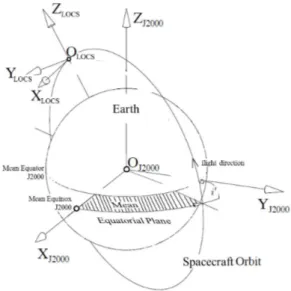
2.2 Coordinate and reference systems . . . . 17

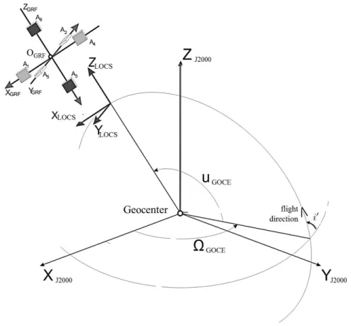
2.2.1 Geocentric, non-rotating reference system . . . . 17

2.2.2 Geocentric, rotating coordinate systems . . . . 18

2.2.3 Local coordinate systems . . . . 21

2.3 Gravity as force and potential . . . . 22

2.3.1 Physical background . . . . 22

2.3.2 Resources for mathematical description . . . . 24

2.3.3 Gravitational potential . . . . 26

2.3.4 Normal potential and gravity . . . . 27

2.3.5 Disturbing potential . . . . 29

2.4 Field transformations . . . . 29

2.4.1 Meissl scheme . . . . 30

2.4.2 Spherical derivatives of the (differential) gravitational potential in terms of SHs . . 32

2.5 Gravitational functionals . . . . 34

2.5.1 Gravitational potential difference . . . . 35

2.5.2 Geoid undulation . . . . 35

2.5.3 Quasigeoid undulation . . . . 36

2.5.4 Gravity disturbance . . . . 37

2.5.5 Gravity anomaly . . . . 37

2.5.6 Deflection of the vertical . . . . 38

2.5.7 Gravity gradients . . . . 39

2.6 Height definitions . . . . 40

2.7 Free-air reduction . . . . 41

3 Measurement systems, models and data 43 3.1 Measurement systems . . . . 43

3.1.1 Terrestrial gravimetry . . . . 44

3.1.2 Ship- and airborne gravimetry . . . . 46

3.1.3 Satellite altimetry . . . . 48

3.1.4 GOCE satellite gradiometry . . . . 50

3.1.5 GRACE satellite mission . . . . 56

3.1.6 CHAMP satellite mission . . . . 59

3.1.7 Swarm satellite mission . . . . 60

3.1.8 Satellite Laser Ranging . . . . 60

3.2 Models . . . . 60

3.2.1 Reference ellipsoids and normal potential models . . . . 61

3.2.2 Global SH gravity field models . . . . 61

3.2.3 Regional model: GCG2011 . . . . 63

3.3 Data . . . . 63

3.3.1 Terrestrial data set . . . . 63

3.3.2 Shipborne data set . . . . 64

3.3.3 Airborne data sets . . . . 65

3.3.4 Altimetry data . . . . 65

3.3.5 GOCE SGG data . . . . 66

3.3.6 GRACE level 2 data . . . . 67

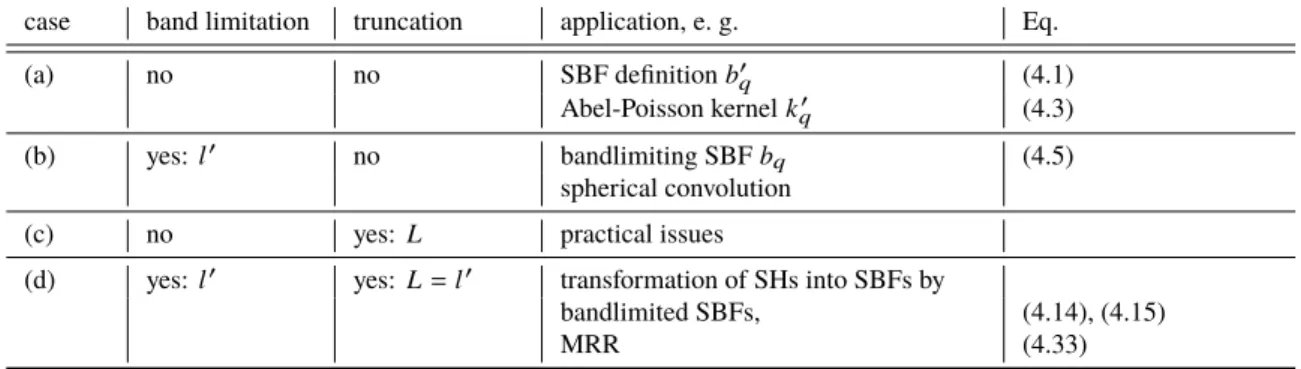
4 Spherical basis functions and multi-resolution representation 69 4.1 Series expansion in terms of SBFs . . . . 70

4.1.1 SBF: definition and properties . . . . 70

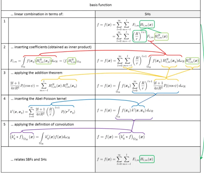
4.1.2 Relation to SHs . . . . 72

4.2 Band limitation . . . . 73

4.2.1 Bandlimiting SBF . . . . 73

4.2.2 Filtering by convolution . . . . 73

4.2.3 Truncation of series expansions . . . . 75

4.2.4 Modeling errors and energy content . . . . 78

4.2.5 Gravitational functionals in terms of SBFs . . . . 80

4.3 Multi-resolution representation . . . . 81

4.3.1 Definition of spectral and spatial resolution . . . . 82

4.3.2 Discretization of the frequency spectrum . . . . 83

4.3.3 Multi-resolution (de)composition . . . . 83

4.3.4 Types of bandlimiting SBFs . . . . 86

4.3.5 Spectral filtering by scaling and wavelet functions . . . . 88

5 Methodical settings, estimation model and spectral combination 93 5.1 Methodical settings . . . . 93

5.1.1 Computation grid and global rank deficiency . . . . 94

5.1.2 Definition of regional target, observation and computation area . . . . 96

5.1.3 Choice of area margins . . . . 97

5.1.4 Estimate of the regional rank deficiency . . . . 97

5.1.5 Choice of modeling resolution . . . . 98

5.1.6 Choice of background model . . . . 101

5.2 Estimation model . . . . 102

5.2.1 Gauß-Markov model . . . . 103

5.2.2 Extended Gauß-Markov model . . . . 105

5.3 Spectral combination via MRR . . . . 109

5.3.1 Analysis and choice of observation groups . . . . 109

5.3.2 Synthesis and spectral composition . . . . 112

6 Results, Validation and Discussion 115 6.1 Single-level approach . . . . 116

6.1.1 Simulation studies . . . . 116

6.1.2 Real data studies . . . . 132

6.2 Spectral combination via MRR . . . . 146

6.2.1 MRR decomposition . . . . 147

6.2.2 MRR composition . . . . 151

7 Summary and Outlook 163

Abbreviations and Nomenclature 171

List of Figures 177

List of Tables 179

Bibliography 181

Appendices 187

A Supplementary theory . . . . 187

B Supplementary numerical studies . . . . 191

1 Introduction

In which direction does a river flow? – Where on Earth is the height ”zero“? – What can we use as reference?

If we try to explain the need of gravity field determination in our daily live, such questions may provide food for thought: we use the Earth’s gravity field as reference for many practical applications. Precise height systems e. g., deliver the basis for engineering or mapping a country. In order to relate all height measurements to a so-called ”zero-height“, a global reference is indispensable – we therefore use gravity. Besides geodetic applications, many neighboring disciplines – especially in geophysics – require gravitational information as well, e. g. to model the Earth’s interior.

Due to density variations on the Earth’s surface, above in the atmosphere, and beneath in the interior, the gravity varies in different regions: Mountains, glaciers, water storage on land, or underwater ridges in the oceans, for instance, have diverse density features. Consequently, their heterogeneously distributed masses cause different gravitational attractions, and turn the determination of the gravity field into a very complex and demanding task.

Motivation

In this work, the main focus is on the determination of the gravitational force on the Earth’s surface, that varies from point to point. The primary aim is determining regional gravity fields as comprehensively, effectively and accurately as possible: The challenge is to develop a flexible regional approach combining any kind of real gravity data in order to deliver medium- up to high-resolution gravity field models. Hereby the overall motivation of setting up a ”regional“ approach – in contrast to a ”global“ one – directly results from the way how to measure the Earth’s gravity field:

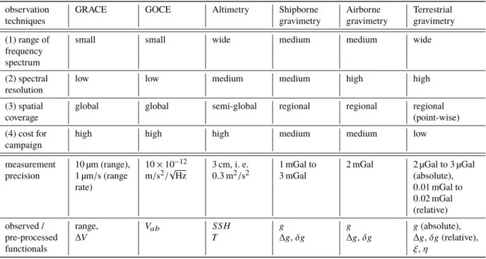
Why do we need regional in addition to global gravity field modeling? A variety of gravity measurement techniques has been developed over the last centuries, which are completely different in their spectral and spatial resolution, accuracy and geographical coverage. Each sensor type has its very specific advantages and disadvantages: Satellites detect the gravity field globally and capture long wavelengths, but the spatial resolution at the Earth’s surface is actually limited down to around 100 km due to the attenuation of the gravity field with increasing altitude. In contrast, local measurement campaigns with terrestrial, air- or shipborne gravimeters are able to detect much finer gravitational structures and deliver spatial resolutions of less than a few kilometers. While satellite observations are the main data source for global gravity models, higher-resolution observations are needed for regional refinements. Spherical Harmonic (SH) functions are established as appropriate tool for global applications, but they capture the high-resolution information of regional, heterogeneous data insufficiently. They suffer the loss of accuracy due to data gaps, different data density and quality. Here, regional approaches come into play: As the high-resolution data sets are available only in a very few parts on Earth, there is an urgent need of regional models, that approximate their invaluable information. Spherical (radial) basis functions (SBF) have global support, but a localizing character. They shall be used to capture spatially limited information and express it with high efficiency and concentration. Being both spatially and spectrally as close as possible to the observations thus requires an appropriate adaptation and set up of the functions. Figure 1.1 presents the general idea.

What are the challenges of (regional) gravity modeling approaches? Localizing Spherical Basis Function

(SBF)s seem to be an appropriate tool for regional gravity modeling, but there are a lot of open questions and

several challenges which have to be studied: After Newton, the Earth’s universal gravitation defines a global

gravity field, so that local data sets and regional models capture by nature only a finite part of the gravitational

signal, i. e. from the spatial point of view, functions with global support fit regionally limited data sets only

Figure 1.1: General idea: Modeling regional gravitational structure (depending on mass distribution) – from real (terrestrial, air- /shipborne, altimetry, GOCE, GRACE, ...) and pseudo (SH model) observations – in terms of SBFs (on top of a global SH model).

The light-blue colored background visualizes the parts which are included in the estimation model, realized in this work.

approximately, and edge effects appear. From the spectral point of view, the Earth’s gravitational potential is a continuous quantity, which theoretically could be described by series expansion up to infinity. However, on the one hand, for practical implementation series expansions have to be limited to a finite number of terms.

The cut of the infinite series expansion always provokes a truncation error; it has to be studied both in regional and in global approaches. On the one hand, the spectral content, i. e. the captured gravitational information of observations is also limited. According to these spectral restrictions, unknown series coefficients have to be determined. Typically parameter estimation is used in geodetic applications (Koch, 1999). In mathematical applications, as for instance presented by Michel (2013), numerical integration is favored. It enables the direct computation of the coefficients based on a quadrature method (Driscoll and Healy, 1994). However, estimating the unknown parameters in the overdetermined problem of regional gravity modeling has several advantages for the task of this work: Error (co-)variances of the model parameters are estimated as well, and thus, the accuracy and precision of the resulting models can be evaluated. Using the observations at their original positions avoids additional error influences, e. g. from interpolation procedures, and enables the combination of data with different resolutions, accuracies and distribution. However, some effort is required to receive a stable solution: Especially inhomogeneously distributed observations due to data gaps and the need of downward continuation processes for measurements obtained in different heights cause a bad condition of the normal equation system. Therefore regularization schemes have to be implemented, e. g. by introduc- ing prior information. In terms of regional modeling approaches using SBFs, the choice of an appropriate regularization strategy is much more sensitive and less investigated than in global approaches. Above all, the variety of basis functions (splines, wavelets, Slepians, Mascons, etc.) offers many positive features, but the selection for different applications and requirements has to be taken very carefully. Open questions append, as e. g. where to locate the functions (on a sphere, ellipsoid, on different layers inside the Earth, etc.), on which kind of point grid (geographical, Reuter, icosahedra grid, etc.), and how to determine and handle the related rank deficiency problems. The establishment of an appropriate adjustment model offers several possibilities how to combine the inhomogeneous data sets, how to implement field transformations of the observed gravity functionals and how to estimate the unknown series coefficients (e. g. by Variance Component Estimation (VCE), Least Squares Collocation (LSC), etc.). All the selections influence each other and have to be taken into account - as well as the model errors from the truncation of the series expansion, from leakage problems, and edge effects.

֒ → The primary aim of this thesis is to investigate all those challenges and to develop a proper, stable and

efficient approach, that delivers accurate, high-resolution regional gravity field models.

What are the benefits of a combination of multiple data sets via MRR? Within this approach, the spectral content of the regional models shall be enhanced by combining the different high-, medium-, and low-resolution data sets as optimally as possible. The long wavelengths of the gravity field and thus, large-scale structures of the Earth, can only be observed by global satellite observation systems, while short wavelengths are mainly detected with high accuracy by local observation systems. The idea is to combine the different data sets in specific regions in such a way that their benefits contribute as much as possible to the gravity field models.

A spectral approach, introducing the resolution-depending gravity information of the different measurement systems step-by-step to the regional model, shall deliver a Multi-Resolution Representation (MRR)

of the resulting gravity signal.

As visualized in Fig. 1.1, the combination model is set up by a global, low-pass filtered SH model (in terms of prior information), and several regional, consecutively band-pass filtered SBF models (supplied by different gravity data sets). Hereby, the observation techniques shall contribute information exactly in the spectral domain of their highest sensitivity, in order to exploit their content and accuracy as optimally as possible, but, as well, by means of reducing erroneous effects as efficiently as possible. The consistent spectral composition of the low- and band-pass filtered gravity field representations can be guaranteed by an appropriate mathematical approach based on a level-discretization of the frequency domain. Furthermore, the connection of the so-called resolution levels could be realized by a pyramid algorithm, which is, however, not part of this thesis. Vice versa, the resulting model can be decomposed by MRR, i. e. displayed at different resolution levels. Viewing a gravitational signal under different resolutions enables to detect valuable features of different spectral domains of our planet, such as groundwater storage, oil reserves or density layers in the interior of the Earth.

Review of different regional gravity modeling approaches

While for global gravity field modeling, the use of SHs is well-established and physically proven, they are less appropriate for high-resolution regional gravity field modeling. SHs are optimally localizing in the spectral domain and due to their global character ideally suited for representing globally distributed data sets. However, if high-resolution data sets are only available in certain geographical regions, the spectral information might not be optimally caught: The leakage of high-resolution spectral information in unobserved areas has to be taken into account which leads to a reduced accuracy of the modeled signal. To optimally exploit the content of regional data sets, various regional modeling approaches have been proposed and further developed, especially during the last two decades. They all have different advantages, challenges and are accordingly appropriate for different applications. In the following, a short overview of the most established methods, their originating idea and their main advantages is given. Table 1.1 lists and categorizes the specific features by means of the exemplary implementation by one research group. The main differences result from the type of basis function that is used:

Spherical basis functions and multi-resolution representation Within the set of basis functions, which also includes SH functions, the regional gravity field community makes use of spherical, i. e. radial basis functions. Freeden et al. (1998) (and many other publications from his working group) provide the fun- damentals of this approach, e. g. further adapted by Schmidt et al. (2007). Altogether the functions are based on Legendre polynomials and thus ensure the solution of the Laplace equation in a global case. In contrast to SHs, the SBFs are isotropic and characterized by their localizing feature. For this reason they are an appropriate tool for regional approaches to consider the heterogeneity of data sources (satellite, airborne, terrestrial, etc.), resulting from a different frequency content, sampling geometry, and observation stochastic.

They are typically located on point grids and the related unknown coefficients which have to be estimated, feature a geophysical meaning by representing the rough structure of the signal that has to be modeled in the end. The choice of several specific parameters is justified by the findings of Bentel et al. (2013b) and Naeimi (2013). Bentel et al. (2013a) studied various different radial basis functions for their application in regional gravity modeling, based on the approach of Freeden et al. (1998) and Schmidt et al. (2007), using scaling or wavelet functions. Those scale-discrete functions act as low- or band-pass filters and thus allow extracting specific domains of the frequency spectrum; from the practical numerical side, they allow implementing fast computation algorithms. Wavelets on the sphere have been studied in detail e. g. by Holschneider M. (1996);

Freeden et al. (1998); Klees and Haagmans (2000).

1In the literature also known as Multi-Scale Representation (MSR), e. g.Freeden(1999);Freeden and Michel(2001).

Due to the different spectral content of complementary observations techniques, Haagmans et al. (2002) and Schmidt et al. (2006) use the advantage of the scale-discretion and set up a MRR by combining a low-pass filtered global geopotential model with band-pass filtered satellite gradiometer and regional high-pass filtered gravity data. In view of a mathematical formulation as suggested by Freeden et al. (1998), the MRR decom- poses the target function into several band-pass filtered detail signals, each related to a certain frequency band and resolution level (e. g. Schmidt et al., 2007). Whereas Schmidt and Fabert (2008) applied the MRR in a top-down scenario by using a pyramidal algorithm, Wittwer (2009) defines a MRR as a bottom-up approach.

Following the concept of adapting SBFs to the frequency content of the signal under investigation, prior variances of the expected signal can be used to construct so-called spherical splines (Eicker, 2008; Eicker et al., 2013). Those kernels allow a high fine-tuning to the signal characteristics and are strictly positive definite, so that the problem is always uniquely solvable (Michel, 2013, p. 163). Further, the properties of the kernels are independent of the chosen point grid on which they are defined, and thus can be placed very flexibly in any region of interest.

Multipole wavelets In contrast to the previous discussed scale-discrete wavelet functions, Panet et al. (2006) use Poisson multipole wavelets. The principle idea to create different scales, i. e. resolution-depending sen- sitivities, is, to locate the sources at different depths (Holschneider et al., 2003). Hereby, the scale corresponds to the distance of multipoles (which are based on series expansion in terms of Legendre polynomials) to the Earth’s surface. Thus, multipoles can physically be interpreted as masses in the Earth’s interior. The main advantages are their locality in phase which leads to quasi-diagonal matrices that are easy to invert, and their definition in the whole space which supports especially the combination of heterogeneous data at different altitudes (Panet et al., 2006). The research groups using multipole wavelets further distinguish between a set of analysis coefficients defined either on a discrete sequence of scales, each containing a fix set of positions, or on different scales and positions as well. The latter method enables a higher spatial flexibility but the computation is much more time consuming.

Mascons The principle idea of simulating mass concentrations that cause differences in the gravitational potential, is applied in the approach of Mascons by Rowlands et al. (2005). The region of interest is modeled by a uniform layer of mass, e. g. a spherical cap or block, which is added to a mean field. Thus, the variations between the mass elements are scaled by differential potential coefficients (Chao et al., 1987) which have to be estimated. Each set of parameters is defined for a specific epoch so that the localization both in space and time is the main advantage of this approach: On the computation side, correlations between regional solutions decrease, and on the application side, regional mass variations and related gravity field changes can be detected very well. As Mascons are optimally adapted to one observation technique, they are not appropriate for combined gravity fields from heterogeneous observation data.

Slepian functions For an optimal concentration of a gravitational signal both in space (or time) and in the spectral domain, Simons (2009) developed an approach using Slepian functions (Slepian and Pollak, 1961).

Those functions are defined within a geographical domain and within a certain frequency bandwidth. The maximum spatial concentration of the strictly band-limited functions in a specific circular region can be found by the maximum energy ratio to respective functions on the whole sphere. The Slepians thus are based on an orthogonal set of SHs and the related unknown “concentrated” coefficients are obtained from the eigenvalue equation of the maximum energy ratio.

Least Squares Collocation The statistical method of LSC has been developed in the 1970s and 1980s (Krarup, 1969; Moritz, 1978; Koch, 1977). The aim is to find the most accurate approximation results on the basis of the available noisy or noise-free data (Moritz, 1972), e. g. approximating stochastic variables in a stochastic process or observed functionals of the Earth’s gravity field (Tscherning, 2015). Compared with the previous mentioned approaches, the use of LSC for regional gravity modeling is the eldest and most experienced. It combines filtering of the input data by removing erroneous noise, adjustment of the unknown parameters, and prediction of a signal, i. e. computing a functional at any desired point. One of the key advantages is, that it provides together with regional gravity field and geoid models from different gravity data types, error information in the form of full covariance matrices. The covariances are assumed to be known and describe the relation between observations and output quantities. For instance Pail et al.

(2009) and Arabelos and Tscherning (2010) adapted the approach for regional refinements of global gravity

models and Tscherning and Arabelos (2011) developed a powerful software package for regional gravity

field determination. Reguzzoni and Sansò (2012) discuss in detail a possible method for the combination of

high-resolution and satellite-only gravity field models.

1 1

(Freeden et al., 1998) (Holschneider et al., 2003) (Chao et al., 1987) (Slepian and Pollak, 1961) (Krarup, 1969) Realization e. g. Scaling functions

by Schmidt et al. (2006), Splines by Eicker et al. (2013)

e. g. Poisson wavelets by Panet et al. (2006)

e. g. block Mascons by Rowlands et al. (2005)

e. g. by Simons (2009) e. g. by Pail et al. (2009);

Tscherning and Arabelos (2011)

Basis Legendre polynomials Legendre polynomials Legendre polynomials Legendre polynomials Legendre polynomials

Unknowns Scaling coefficients scales Mascon parameters: scale

factor on the set of differential coefficients

eigenvalues coefficients of prediction

Location/ spatial reference of unknowns

Reuter grid

(equidistributed grid points on a sphere, on the Earth’s surface or above)

Icosahedron

(hierarchical icosahedral meshes on spheres with different radii, in the Earth’s interior)

geographical blocks (e. g.

4

× 4

) on a sphere, on the Earth’s surface, beneath or above)

spherical area, defined by center and radius, on the Earth’s surface

input data

Adjustment model and regularization

extended Gauß-Markov Model (GMM), using VCE;

prior information from a global SH model

geometric progression of scales; forward modeling with Gaussian probability (least squares);

prior information by using a generalized inverse

estimation of Mascon parameters;

constraints between Mascons that are close in space and time

estimating eigenvalues from the maximum energy ratio between spatially and spectrally localizing and global functions;

inverse problems linear in the data: truncated Slepian basis (at Shannon number, i. e. sum of eigenvalues)

least squares adjustment by expressing the relation between observations and output signal through covariances

consideration of model errors/

(in)completeness

error propagation including signal (truncation error) and noise

covariance matrix of data noise; covariance matrix of coefficients

correlations between the Mascons w.r.t. signal

noise covariance direct computation of covariances between

observations and output signal Advantages and

disadvantages

(+) highly localizing, (+) strict band limitation possible,

(-) oscillations due to spatial truncation

(+) defined in the whole space (+) quasi-diagonal matrices easy to invert,

(-) non-band limited, non-compact support

(+) high localization both in space and time (high resolution models),

(+) direct gravity computation (no truncation errors from any conversion to SHs),

(-) prior information: strong spatial constraints

(+) optimal spatial and spectral concentration,

(+) reduced number of functions,

(-) numerical instabilities due to small eigenvalues

(+) full covariance information directly provided

(+) flexible for combination of any observation data

(-) large equation systems to solve (depending on number of observations)

Examples of prominent (gravity field or further) applications

height systems, detection of data gaps, ...

3D analysis of the Earth’s interior, lithosphere structure studies, geoid models, ...

mass variations on land (glacier), in the ocean, surface water variations, ...

localized gravitational (mass change) or geomagnetic anomalies, ...

static, combined, regional

gravity field models, ...

In Fig. 1.2, the basis functions are arranged w.r.t. their spectral and spatial localization property. According to the uncertainty principle a perfect localization both in the spectral and in the spatial domain is not possible. While the SHs are optimally localizing in the spectral domain, the Dirac function (visualized as infinite small peak) is optimally localizing in the spatial domain. Consequently, SHs are appropriate for representing the signal of globally distributed data, while the Dirac function would optimally represent the signal measured at a single point.

In order to represent the signal of geographically limited regions, the above presented regional approaches (except the method of LSC) use basis functions, which are all a compromise in-between an optimal spatial and spectral localization (Freeden et al., 1998).

Figure 1.2: Schematic arrangement of basis functions w.r.t. their spectral and spatial lo- calization property.

Altogether, the resulting regional models are not able to resolve the low parts of the frequency spectrum from spatially limited observation sets. In order to cover a broad range of the gravity field signal and to optimally exploit the strengths of each approach, the chosen regional model e. g. can be placed on the top of a high accurate global gravity model, usually based on global satellite observations modeled by SH basis functions.

Hereby, satellite-only combination models, such as the Gravity Observation COmbination (GOCO) series (Pail et al., 2010) including data from Gravity Recovery And Climate Experiment (GRACE), from Gravity field and steady-state Ocean Circulation Explorer (GOCE), and from other satellite-related data sources, are distinguished, as well as combination models, such as Earth Gravitational Model 2008 (EGM2008) (Pavlis et al., 2012) including terrestrial and altimetric gravity field data. The latter enhance the spatial resolution apparently on a global scale, but in fact only in regions where a reasonable terrestrial data basis is available.

Research objectives

In this thesis a method of regional gravity field modeling is presented from the combination of various observation techniques via MRR, that enables on the one hand to extract the maximum spectral content out of each measurement system, and on the other hand to manage different observation positions, accuracies and resolutions. Hereby, the focus is on a flexible approach for the combination of real data considering all their specific features, by enhancing the approach of Spherical basis functions. This leads to the first research objective, handled in this thesis:

1. Developing a regional modeling approach using SBFs

Why are SBFs appropriate functions for regional modeling? The main advantage of SBFs in contrast to SHs is their highly localizing character. Both types of globally supporting basis functions are developed in series expansion based on Legendre polynomials. As SHs are eigenfunctions of the Laplace operator (Freeden et al., 1998, p. 36), they are the best choice for gravity field modeling approaches from data with full global coverage. The resulting model of the gravitational potential satisfies the Laplace condition and thus has a physical meaning. Further, the series expansion can be adapted very flexibly to any kind of observation type, e. g. to various gravitational functionals or to measurements at different heights, by applying field transformations. Thus, they are an excellent tool for the combination of different data sets.

Since SBFs and SHs can be related to each other, gravity field solutions in SHs can be transformed into solutions in terms of SBFs and vice versa. Consequently, global gravity field modeling by SBFs makes use of all positive (and negative) features of the well-established SH approach. However, for regional application of SBFs, several additional challenges have to be considered, as e. g. the handling of rank deficiencies, edge effects, truncation errors, etc.

What are the advantages of the SBF approach compared with other regional approaches? The task is,

to implement a regional modeling approach which manages the difficulties of SBFs and takes their benefits,

compared with and as an alternative to other regional approaches, especially in terms of combining different

data sets (see 2. objective). For this case, the spectral flexibility of the functions shall be exploited: acting

as low- and band-pass filters they allow an adaptation to the spectral content of the observation data, as exactly as it is known. Spatially, they can be adapted very flexibly to the observations as well, e. g. by locating their origins anywhere within the appropriate area at the Earth’s surface, or along satellite tracks.

The resulting challenge is here, to balance the localization in spatial and spectral domain. As a strict band limitation, i. e. an exact frequency cut, enables the spectral combination of different data sets at appropriate resolution levels, a MRR can be applied to construct the output signal. This unique feature of the SBF approach enables to realize the second objective of this work:

2. Combining different data sets via MRR as optimally as possible

What is the additional value of a combination? As the different measurement systems are sensitive in different frequency domains, they deliver data with different spectral resolutions. In order to model the gravitational signal as completely and as highly resolved as possible, the maximum information of the observations shall be exploited.

Why is MRR an appropriate combination tool? A close to optimum spectral combination can be achieved by MRR: the frequency domain is split into several resolution levels and the appropriate gravitational signal is modeled from the data obtained by the measurement techniques which are sensitive in this bandwidth.

Adding the so-called detail signals in the end, delivers the full gravitational signal between the lowest and the highest resolution of all contributing observations. Missing long wavelengths parts can be filled up with information from global models. Thus, not only a high-resolution regional gravity model is obtained containing as much spectral content as possible, but also information depending on the spectral resolution can be derived from the single detail signals. Different geophysical processes have different spectral sensitivities; potential relations could be derived from such a MRR of the gravitational signal.

Vice versa to the bottom-up approach, any final gravitational signal could be set up by a top-down algorithm as well, starting with the highest-resolution data set and introducing step-by-step lower-resolution observations. Schmidt et al. (2015) theoretically described such a pyramid algorithm by computing the lower levels not only from new observations but also by using the information of the higher levels, considering potential correlations. In this work the bottom-up approach is presented due to its much easier implementation.

3. Enhancing the approach for the use of real data

What can we learn from simulation studies? Besides real input data, simulated data, e. g. functionals computed from a global SH model, can be used to estimate gravitational signals. Comparing finally the resulting output model with the input model completes the so-called ”closed-loop“ scenario. The aim is to minimize the differences between in- and output. As the input data and comparison data relate to the same origin, the differences answer two questions: (1) How accurately does the regional approach fit the real data? (2) Are the chosen modeling parameters and settings appropriate? Simulating observations in different heights or at different noise levels, approximates the characteristic of real data more and more and enables to indicate the stability of the approach.

What are the challenges of real data? As in most cases the stochastic of real observations is just poorly known, the objective of this work is to develop the approach at the same time as robust and flexible as possible. Especially data gaps and missing knowledge of the exact frequency content of the measurements are additional challenges that have to be considered.

Depending on the application, the selection of data sets and/or the choice of the region have to be made:

The availability, the height, the type, the accuracy, the spatial and the spectral resolution of the data are important criteria, further, the type and resolution of appropriate prior information in order to close data gaps, and finally the location and size of the area to be modeled – depending on the data coverage, edge effects and desired spectral resolution of the resulting gravity signal. As the focus of this work lies on the combination of various different measurement techniques, the regional gravity modeling approach shall not be enhanced in the sense of finding the best model fit to each single data set, but in the sense of finding an optimal fit in order to extract as much information as possible, i. e. to take benefit from all data sets.

All the challenges, mentioned in the last point, shall be studied and considered – together with the findings from simulation studies – in order to reach the first two objectives. This leads to the overall topic of this thesis:

Enhanced regional gravity field modeling from the combination of real data via MRR.

Outline

The thesis is structured in seven main Chapters (including the Introduction). Each Chapter is divided and subdivided in several sections.

Chapter 2 The fundamentals are presented in Chapter 2. They contain both, the study of appropriate lit- erature, but as well, based on appropriate literature, further development of relations which are relevant and important for this work. In the first two sections, Sec. 2.1 and Sec. 2.2, the underlying spaces, dimensions, bases, and coordinate systems are defined. They span the mathematical background. Section 2.3 introduces the physical background. Gravity and gravitational potential are described under the modeling aspect, together with their well-known representation in terms of SHs using Legendre functions. Hereby, new aspects are derived, since the here presented regional gravity modeling approach is established on Legendre Polynomials.

Further, field transformations in Sec. 2.4 are studied in order to relate various gravitational functionals under the aspect of their spectral sensitivity. A selection of gravity related quantities, obtained from first and second order derivatives of the potential, is finally presented in Sec. 2.5. Relevant height definitions and reductions complete this chapter.

Chapter 3 The different functionals stem from a variety of measurement systems. They are presented in the first part, Sec. 3.1, of Chapter 3. In Sec. 3.2, a selection of existing models, computed from observables of diverse measurement systems, are presented. In this thesis, global models serve as reference for regional observation techniques, as reference for regional models according to Fig. 1.1, and for regularization pur- poses. From comparisons of the here computed regional and other regional or global gravitational models, the approach can either be validated, or different information can be identified. In Sec. 3.3 the specific data sets used in this work, and their pre-processing are described. Since the aim is to extract as much information as possible from the measurements, the observations shall be kept in their most original and less pre-processed state.

Chapter 4 The fundamentals of the regional modeling approach are formulated in Chapter 4. It thus com- prises the core of this work. In Sec. 4.1, the SBFs are introduced and related to SH basis functions. From theoretical investigations of representing non-bandlimited functions, in Sec. 4.2, the transition to bandlimiting SBFs is discussed. Spherical convolution and referring filtering characteristics are the key elements. Further, the truncation of series expansions and corresponding errors are discussed. Finally, the SBFs are adapted to various gravitational functionals. In the third part, Sec. 4.3, the principle of MRR is introduced. The favorable filtering characteristics of SBFs are used for representing signals at different spectral resolutions.

The framework for the MRR is hereby an appropriate splitting of the frequency spectrum into resolution levels.

Chapter 5 Another key role in this work plays Chapter 5. In the first part, Sec. 5.1, several tools and settings for establishing the enhanced regional gravity modeling approach are presented. Hereby, a kind of “recipe”

is given for a reasonable, well-balanced parametrization. Especially restricting investigations from global gravity field representations to regional applications are discussed in detail. In the second part, in Sec. 5.2, the estimation model is set up. It is subdivided into a single-level estimation method, computing gravitational functionals from a combination of various observations in specified regions at one resolution level, and a multi-level estimation method, presenting the spectral combination at different resolution levels within the framework of a MRR.

Chapter 6 In Chapter 6, the enhanced regional modeling approach is applied to numerical studies. Besides presenting the results, classified in a variety of different study cases, different methodical parametrization is discussed. Hereby, the complexity increases with investigating a larger number of influencing factors. In principle, two categories are distinguished: Section 6.1 investigates results from the single-level estimation model, while Sec. 6.2 investigates results from the spectral combination model via MRR. First of all, within simulation studies, the stability, consistency and efficiency of the approach shall be judged and verified. Based on those findings, real data studies are discussed with the aims of computing high-resolution regional gravity fields, and regionally refining existing global models. The beneficial peculiarities and the potential of the MRR approach are compared with the single-level approach. Due to the large diversity, only a selection of results can be studied. Within the different study cases, different error influences are identified and discussed in detail.

Chapter 7 The benefits, compromises, and weaknesses of the enhanced regional gravity modeling approach

are finally summarized in Chapter 7. With recommendations and ideas for further studies, this thesis closes.

2 Fundamentals

The Earth’s gravitational potential V , resulting from attractions between masses, delivers together with the centrifugal potential Z, resulting from the Earth’s rotation, the total gravity potential W = V + Z. From any potential equipotential surfaces can be derived, i. e. surfaces with constant potential. According to this is favorable property, the ”geoid“ is the most important equipotential surface in geodesy. Its according potential W = W

serves as mathematical description of the figure of the Earth (Hofmann-Wellenhof and Moritz, 2005, p. 47), i. e. it is ideally suited for many geodetic applications, such as providing a reference for height systems.

The gravitational potential V is the fundamental quantity for all following considerations in this thesis due to several reasons: From the mathematical point of view, this scalar potential satisfies the Laplace equation and can be expressed as harmonic function outside the Earth’s attracting masses. Consequently, essential advantages are inferred for modeling and measuring aspects: A variety of gravitational functionals, as e. g.

gravity gradients, gravity anomalies or geoid heights can be derived from the (differential) potential. As mentioned, it further allows to quantify equipotential surfaces. Those unambiguous, well-observable surfaces deliver the basis for detecting density, i. e. mass variations at the Earth’s surface.

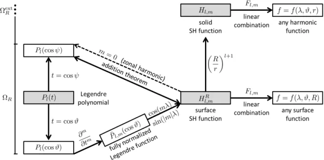
The following sections give an overview of all gravity related quantities used in this work: Definitions, derivations and relations shall be explained. Special emphasis is given on the way how to describe the gravitational quantities by functional models for the global case. Hereby SHs are used as most popular basis functions. The fundamental part of all basis functions regarded in this thesis are Legendre polynomials. They and their derivatives are the key elements of the later adapted SBFs. Further, this chapter identifies common features between SHs and SBFs. It is, thus, a mixture of reviewing relevant literature, but in equal measure deriving new relations, which contribute to the basis for setting up the regional modeling approach in Chapters 4 and 5, the core of this work.

The chapter is structured as follows: First of all, the underlying spaces, dimensions, bases, and coordinate systems are introduced, spanning the mathematical background. Second, gravity and gravitational potential are introduced under the modeling aspect, together with their well-known representation in terms of SHs using Legendre functions. From the modeling perspective, normal and disturbing potential are briefly introduced, as well. The field transformations in the third part establish the relations between various gravitational functionals.

The Meissl scheme hereby provides a reasonable structure and is extended to the specific requirements in this work. A selection of gravity related quantities, obtained from first and second order derivatives of the potential, is finally presented in the fourth part. Some remarks on related height definitions and reductions used in this work complete this chapter.

2.1 Spaces, dimensions and bases

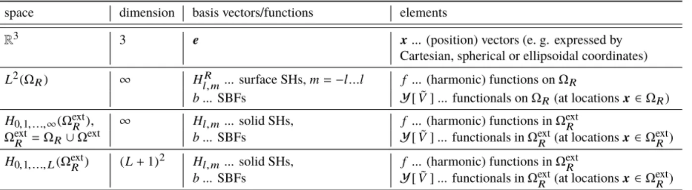
In this work, all coordinate systems and functions are determined in relation to vector spaces and only real valued functions are used. Table 2.1 gives an overview of the relevant spaces, examples for their basis and elements used here. The structure of this section follows the table, starting with describing vectors in the well-known Euclidean space, transferring the investigations to the description of functions/functionals on a sphere, and finally describing elements in the exterior of a sphere, as well.

Vector space

The coordinate systems are defined in the metrical, three-dimensional Euclidean space R

(e. g. Heinhold

and Riedmüller, 1971, pp. 79). It needs exactly three non-collinear basis vectors e ∈ R

(here e

, i ∈ { 1, 2, 3 } )

to span this vector space. Any element, e. g. the position vector x ∈ R

, is uniquely defined within R

and

Table 2.1: Overview of spaces, their basis vectors/functions, and exemplary elements.

space dimension basis vectors/functions elements

R

3 e x ... (position) vectors (e. g. expressed by

Cartesian, spherical or ellipsoidal coordinates) L

( Ω

) ∞ H

... surface SHs, m = − l...l f ... (harmonic) functions on Ω

b ... SBFs Y [ ˜ V ] ... functionals on Ω

(at locations x ∈ Ω

) H

( Ω

), ∞ H

... solid SHs, f ... (harmonic) functions in Ω

Ω

= Ω

∪ Ω

b ... SBFs Y [ ˜ V ] ... functionals in Ω

(at locations x ∈ Ω

) H

( Ω

) (L + 1)

H

... solid SHs, f ... (harmonic) functions in Ω

b ... SBFs Y [ ˜ V ] ... functionals in Ω

(at locations x ∈ Ω

)

can be expressed as linear combination of the three basis vectors, i. e.

x = X

i=1

x

e

. (2.1)

Each component x

(coefficient, linear factor, respectively) can be interpreted as scaling factor of a projection of x onto e

.

If the basis vectors are unit vectors and orthogonal to each other (e. g. e

= (1, 0, 0)

, e

= (0, 1, 0)

, e

= (0, 0, 1)

), they form an orthonormal basis, i. e.

D e

, e

E

R³

= e

e

= δ

, i, j ∈ { 1, 2, 3 } , δ

=   

0 for i , j

1 for i = j (2.2)

k e k

= p

h e, e i

= 1 . (2.3)

In Eq. (2.2) the inner or scalar product is applied on two vectors e

, e

∈ R

; Eq. (2.3) presents the norm of a vector e ∈ R

. In case of orthogonal basis vectors, the elements of the Euclidean space can be described, for instance, by Cartesian coordinates (see Sec. 2.2.2).

Function space

A function f with a certain numerical function value f ( x) at a location with position vector x, is defined in a function space (Lanczos, 1997, p. 166), cf. Tab. 2.1.

... on a sphere: In contrast to the specific finite-dimensional space R

, functions are in the following defined in the L

normed vector space. On a sphere Ω

with radius R and surface elements dω

the space is introduced as L

( Ω

). According to Eq. (2.1), each element, e. g. a function f ∈ L

( Ω

) with x ∈ Ω

f = f ( x) = X

i=0

c

b

( x) , (2.4)

can be expressed by a set of an infinite number of basis functions b

and coefficients c

, i. e. a linear combination of basis functions.

If the scalar product of two basis functions exists, the L

space, also denoted space of square integrable functions, is a Hilbert space. The scalar product of two basis functions b

, b

(cf. Freeden et al. (1998), pp. 57) and the norm of a basis function b read

D b

, b

E

L²(ΩR)

= Z

ΩR

b

(x )b

( x)dω

= : D b

, b

E

ΩR

(2.5)

2In the following, the short formf(x)is used, for instance, for describing a functionf = f(x)in the text, related to the literature. Basis functionsb can either be one-point functions with function valuesb(x)depending onx, or two-point functions withb=b(x,x_q), additionally depending on the location of the function’s center with position vectorx_q.

k b k

=

 

 

Z

ΩR

| b(x) |

dω

 

 

1 2

= : k b k

< ∞ (2.6)

with x ∈ Ω

. For basis functions b

, b

∈ L

( Ω

) spanning an orthonormal base, the scalar product (2.5) becomes δ

=   

0 for i , j

1 for i = j , i, j ∈ N

. Referring to Freeden (1999), p. 39, 81, the spherical convolution of a basis function b and an element f ∈ L

( Ω

) is defined as

( f ∗ b)

(x ) = Z

ΩR

f ( x)b( x)dω

= h f , b i

. (2.7)

It is equivalent to the inner product of f and b, cf. Eq. (2.5). In the sequel of this thesis, basis functions which are used for convolution, are denoted kernel functions or kernels.

... on and above a sphere: Functions which further shall describe properties of the exterior (ext) of a sphere Ω

, i. e. Ω

:= Ω

∪ Ω

, are defined in a space H

( Ω

) (Schmidt et al., 2007). Compared to the L

space, in this expanded space the basis functions b ∈ H

( Ω

) and their linear combinations cannot be orthogonal.

2.2 Coordinate and reference systems

From the motivation of regional gravity field modeling it becomes clear, that the Earth’s gravity field is a position-dependent quantity. But which coordinates are appropriate in order to express the gravitational potential V (or any functional of it) at different locations? For either describing a physical phenomenon within specific models, or for measuring specific quantities, various coordinate systems are indispensable and have favorable characteristics. That is, depending on the geometrical, instrumental or practical problem, different observation techniques rely on their own specific reference systems. In order to observe and describe the dynamic system Earth from space, an inertial reference system is appropriate. Consequently, for gravity field modeling from the combination of various heterogeneously defined observables and their approximation by an appropriate model, transformation equations are needed. The most appropriate systems and their relations, i. e. transformations, to each other are presented in the following sections.

(1) A geocentric non-rotating system, (2) geocentric rotating systems, mainly used for global gravity field representations, and (3) local Earth- and satellite-bound coordinate systems, suitable for specific measurement systems, are distinguished. All systems are defined in the three-dimensional Euclidean space R

.

2.2.1 Geocentric, non-rotating reference system

The fundamental system in which Newton’s physical laws hold, is a non-rotating, inertial reference system.

Such a system is for instance appropriate for describing the movement of Earth-observing spacecrafts, inde-

pendently of the Earth’s rotation.

The satellite missions, from which data are used in this work, relate to a right-handed system specified by the epoch of Julian Date of 2000 (J2000): the origin O

is defined in the center of mass (geocenter), and the axes X

intersection of mean ecliptic plane with the

mean equatorial plane at J2000 (counted positively towards the vernal equinox), Z

orthogonal to the mean equatorial plane at

J2000,

Y

orthogonal to the X

- and Y

-axes, span a right-handed system (Cesare, 2008, p. 11).

The example of the J2000 inertial reference system is shown in Figure 2.1. Within this system, a local oriented reference system (LOCS) is displayed as well

(see Sec. 2.2.3). Figure 2.1: Inertial reference and local orbital coordinate system, adapted from Cesare (2008). i means the inclina- tion angle of the spacecraft orbit.

2.2.2 Geocentric, rotating coordinate systems

For describing phenomena on the Earth, rotating, Earth-bound coordinate systems are appropriate. In contrast to non-rotating, inertial systems, they are non-inertial; apparent (or pseudo) forces apply, as e. g. the centrifugal or the Coriolis force. In order to model gravitational functionals related to the Earth’s surface, the following four Earth-bound, geocentric coordinate systems are most convenient.

Cartesian coordinate system

The fundamental terrestrial coordinate system is defined by 3 rectangular axes X, Y, Z: They span a three-dimensional, right-hand oriented Cartesian coor- dinate system, see Fig. 2.2. (The local north-oriented coordinate system (LNCS), also visualized in Fig. 2.2, will be introduced in Sec. 2.2.3.) The XY Z-system rotates with the Earth and regards all masses, i. e.

solid, fluid, and gaseous ones. The origin is defined in the center of mass. The coordinates of the Cartesian system are specified as

x along the X-axis (intersection of mean equatorial plane and mean meridian plane trough Greenwich),

y along the Y -axis (intersection of mean equatorial plane and meridian plane

orthogonal to the plane through Greenwich), z along the Z-axis (mean rotation axis).

The coordinates x, y, z are counted in metric values.

The location of any point P can be described by P(x, y, z) = P( x) with x = [x, y, z]

; the distance ds between two points is defined by the square root of ds

= dx

+ dy

+ dz

.

Figure 2.2: Cartesian coordinate system with spherical coor-

dinates and local north-oriented coordinate system (LNCS),

adapted from Koop (1993, p. 183).

Spherical coordinate system

As many geodetic problems, computations and applications are formulated and executed on a sphere, spherical coordinates are introduced with

λ geocentric longitude (angle [0

· · · 360

[, measured in equatorial plane, counted positively east-wards from meridian plane through Greenwich)

ϕ geocentric latitude (angle [ − 90

· · · 90

], measured in meridian plane, counted positively

north-wards from equatorial plane to the normal through the corresponding point on the sphere), (ϑ co-latitude, respectively polar distance angle 90

− ϕ [0

· · · 180

], measured in meridian plane,

counted positively south-wards from North to South pole), and r radial distance from the geocenter (counted in metric units),

see Fig. 2.2. A point P(λ, ϕ, r ) = P(x) then can be identified by its geocentric position vector

x = r · r = r · [ cos ϕ cos λ, cos ϕ sin λ, sin ϕ ]

= r · [x, y, z]

. (2.8) Hereby r denotes the unit vector and r = | x | = R + h the radial distance of the point P with height h over the sphere Ω

with radius R. The element of distance ds is now given as

ds

= dr

+ r

dϑ

+ r

sin

ϑdλ

, (2.9)

and the surface element dω

on the sphere Ω

(cf. Sec. 2.1) is defined as

dω

= R

sin ϑdϑdλ . (2.10)

The spherical distance angle ψ between two surface points can be computed by ψ = arccos

cos ϑ cos ϑ

+ sin ϑ sin ϑ

cos( λ

− λ)

(2.11) (e. g. Torge, 2003, p. 60). The origin of the spherical coordinate system is located in the center of mass, equivalently to the origin of the Cartesian system.

Transformation: Cartesian – spherical coordinates The transformation equations from Cartesian x, y, z to spherical λ, ϕ, r coordinates yield

λ = arctan y

x

, ϕ = arctan *

, z p x

+ y

+

- , (2.12)

r = q

x

+ y

+ z

.

Ellipsoidal coordinate system

While approximating the Earth as a sphere is practical or sufficient for many geodetic applications, some

require a more precise approximation: the geometrical figure of a rotating ellipsoid (ellipsoid of revolution,

spheroid) is used, e. g., for national position coordinates or for the normal gravitational potential, which is

described later in Sec. 2.3.4. The deviation from a sphere is expressed by the flattening f

, depending on the

major and minor semi-axes a and b.