Kalman Filtering with State Constraints Applied to Multi-sensor Systems and Georeferencing

Veröffentlichungen der DGK

Ausschuss Geodäsie der Bayerischen Akademie der Wissenschaften

Reihe C Dissertationen Heft Nr. 856

Sören Vogel

Kalman Filtering with State Constraints Applied to Multi-sensor Systems and Georeferencing

München 2020

Verlag der Bayerischen Akademie der Wissenschaften

ISSN 0065-5325 ISBN 978-3-7696-5268-0

Diese Arbeit ist gleichzeitig veröffentlicht in:

Wissenschaftliche Arbeiten der Fachrichtung Geodäsie und Geoinformatik der Universität Hannover ISSN 0174-1454, Nr. 364, Hannover 2020

Veröffentlichungen der DGK

Ausschuss Geodäsie der Bayerischen Akademie der Wissenschaften

Reihe C Dissertationen Heft Nr. 856

Kalman Filtering with State Constraints Applied to Multi-sensor Systems and Georeferencing

Von der Fakultät für Bauingenieurwesen und Geodäsie der Gottfried Wilhelm Leibniz Universität Hannover

zur Erlangung des Grades Doktor-Ingenieur (Dr.-Ing.) genehmigte Dissertation

Vorgelegt von

Sören Vogel, M.Sc.

Geboren am 07.04.1988 in Leimen

München 2020

Verlag der Bayerischen Akademie der Wissenschaften

ISSN 0065-5325 ISBN 978-3-7696-5268-0

Diese Arbeit ist gleichzeitig veröffentlicht in:

Wissenschaftliche Arbeiten der Fachrichtung Geodäsie und Geoinformatik der Universität Hannover ISSN 0174-1454, Nr. 364, Hannover 2020

Adresse der DGK:

Ausschuss Geodäsie der Bayerischen Akademie der Wissenschaften (DGK) Alfons-Goppel-Straße 11 ● D – 80539 München

Telefon +49 – 331 – 288 1685 ● Telefax +49 – 331 – 288 1759 E-Mail post@dgk.badw.de ● http://www.dgk.badw.de

Prüfungskommission:

Vorsitzender: Prof. Dr. Philipp Otto Referent: Prof. Dr.-Ing. Ingo Neumann

Korreferenten: Prof. Dr.-Ing. Hans-Berndt Neuner (TU Wien) Prof. Dr.-Ing. Steffen Schön

Tag der mündlichen Prüfung: 05.08.2020

© 2020 Bayerische Akademie der Wissenschaften, München

Alle Rechte vorbehalten. Ohne Genehmigung der Herausgeber ist es auch nicht gestattet,

die Veröffentlichung oder Teile daraus auf photomechanischem Wege (Photokopie, Mikrokopie) zu vervielfältigen

ISSN 0065-5325 ISBN 978-3-7696-5268-0

Active research on the development of autonomous vehicles has been carried out for several years now. However, some significant challenges still need to be solved in this context. Particularly relevant is the constant guarantee and assurance of the integrity of such autonomous systems. In order to ensure safe manoeuvring in the direct environment of humans, an accurate, precise, reliable and continuous determination of the vehicle’s position and orientation is mandatory. In geodesy, this process is also referred to as georeferencing with respect to a superor- dinate earth-fixed coordinate system. Especially for complex inner-city areas, there are no fully reliable methods available so far. The otherwise suitable and therefore common Global Navigation Satellite System (GNSS) ob- servations can fail in urban canyons. However, this fact does not only apply exclusively to autonomous vehicles but can generally also be transferred to any kinematic Multi-Sensor System (MSS) operating within challenging environments.

Especially in geodesy, there are many MSSs, which require accurate and reliable georeferencing regardless of the environment. This is indispensable for derived subsequent products, such as highly accurate three-dimensional point clouds for 3D city models or Building Information Modelling (BIM) applications. The demand for new georeferencing methods under aspects of integrity also involves the applicability of big data. Modern sensors for capturing the environment, e.g. laser scanners or cameras, are becoming increasingly cheaper and also offer higher information density and accuracy. For many kinematic MSSs, this change leads to a steady increase in the amount of acquired observation data. Many of the currently methods used are not suitable for processing such amounts of data, and instead, they only use a random subset. Besides, big data also influences potential requirements with regard to possible real-time applications.

If there is no excessive computing power available to take into account the vast amounts of observation data, recursive methods are usually recommended. In this case, an iterative estimation of the requested quantities is performed, whereby the comprehensive total data set is divided into several individual epochs. If the most recent observations are successively available for each epoch, a filtering algorithm can be applied. Thus, an efficient estimation is carried out and, with respect to a comprehensive overall adjustment, generally larger observation sets can be considered. However, such filtering algorithms exist so far almost exclusively for explicit relations between the available observations and the requested estimation quantities. If this mathematical relationship is implicit, which is certainly the case for several practical issues, only a few methods exist or, in the case of recursive parameter estimation, none at all. This circumstance is accompanied by the fact that the combination of implicit relationships with constraints regarding the parameters to be estimated has not yet been investigated at all.

In this thesis, a versatile filter algorithm is presented, which is valid for explicit and for implicit mathematical relations as well. For the first time, methods for the consideration of constraints are given, especially for implicit relations. The developed methodology will be comprehensively validated and evaluated by simulations and real- world application examples of practical relevance. The usage of real data is directly related to kinematic MSSs and the related tasks of calibration and georeferencing. The latter especially with regard to complex inner-city environments. In such challenging environments, the requirements for georeferencing under integrity aspects are of special importance. Therefore, the simultaneous use of independent and complementary information sources is applied in this thesis. This enables a reliable georeferencing solution to be achieved and a prompt notification to be issued in case of integrity violations.

Keywords: Recursive State-Space Filtering, State Constraints, Implicit Functions, Georeferencing, Integrity

Bereits seit einigen Jahren wird aktiv an der Entwicklung von autonomen Fahrzeugen geforscht. Allerdings gilt es in diesem Zusammenhang noch einige signifikante Herausforderungen zu lösen. Besonders relevant ist dabei die ständige Gewährleistung und Sicherstellung der Integrität solcher autonomen Systeme. Um ein sicheres Manövrieren in der direkten Umgebung von Menschen gewährleisten zu können, ist eine genaue, präzise, zu- verlässige und kontinuierliche Positions- und Orientierungsbestimmung des Fahrzeuges zwingend erforderlich.

Im Bezug zu einem übergeordneten erdfesten Koordinatensystem wird dieser Vorgang in der Geodäsie auch als Georeferenzierung bezeichnet. Besonders für komplexe innerstädtische Gebiete existieren jedoch noch keine vollumfänglich zuverlässigen Lösungsmethoden. Die ansonsten geeigneten und daher auch gebräuchlichen Beobachtungen eines Global Navigation Satellite Systems (GNSS) können in dieser Hinsicht in engen Häuser- schluchten versagen. Diese Tatsache gilt jedoch nicht nur ausschließlich für autonome Fahrzeuge, sondern lässt sich im Allgemeinen auf jedes kinematische Multisensorsystem (MSS) übertragen.

Gerade auch in der Geodäsie existieren eine Vielzahl solcher MSS, welche eine stets genaue und zuverlässige Georeferenzierung unabhängig von der jeweiligen Umgebung erfordern. Für daraus abgeleitete Folgeprodukte, wie z.B. hochgenaue dreidimensionale Punktwolken für Anwendungen im Rahmen von 3D Stadtmodellen oder Building Information Modelling (BIM), ist dies unverzichtbar. Mit dem Bedarf an neuen Methoden für eine Georeferenzierung unter Aspekten der Integrität, geht zeitgleich auch die Anwendbarkeit von Massendaten einher. Moderne Sensoren zur Erfassung der Umgebung, wie z.B. Laserscanner oder Kameras, werden im- mer preiswerter und weisen zudem in Relation dazu eine immer höhere Informationsdichte und Genauigkeit auf. Dies führt bei zahlreichen kinematischen MSS zu einem stetigen Anstieg der erfassten Beobachtungsdaten.

Viele derzeitige Methoden sind dafür nicht ausgelegt beziehungsweise verwenden stattdessen nur eine zufällige Untermenge der eigentlich verfügbaren Informationen. Zusätzlich beeinflusst dies auch potentielle Ansprüche hinsichtlich möglicher Echtzeitanwendungen.

Steht keine überdurchschnittliche Rechenleistung zur Berücksichtigung der großen Datenmengen zur Verfü- gung, bieten sich in der Regel rekursive Verfahren an. Dabei wird eine iterative Schätzung der gesuchten Größen durchgeführt, wobei die umfassende Gesamtmenge an Beobachtungsdaten in mehrere einzelne Epochen aufge- teilt wird. Liegen aktuellste Beobachtungen sukzessive pro Epoche vor, kann ein Filteralgorithmus angewendet werden. So wird ebenfalls eine effiziente Schätzung durchgeführt und es können in Relation zu einer um- fassenden Gesamtauswertung im Allgemeinen größere Beobachtungsmengen berücksichtigt werden. Solche Filterverfahren existieren bislang jedoch fast ausschließlich für explizite Beziehungen zwischen den verfügbaren Beobachtungen und den gesuchten Schätzgrößen. Ist dieser mathematische Zusammenhang implizit, was durch- aus bei vielen praktischen Fragestellungen der Fall ist, existieren nur sehr wenige Methoden beziehungsweise im Falle der rekursiven Parameterschätzung gar keine. Dieser Umstand geht mit der Gegebenheit einher, dass das Zusammenwirken von impliziten Zusammenhängen mit Restriktionen hinsichtlich der zu schätzenden Parameter bislang noch überhaupt nicht untersucht wurde.

Im Rahmen dieser Arbeit wird daher ein vielseitig einsetzbarer Filteralgorithmus präsentiert, welcher sowohl für explizite als auch für implizite mathematische Zusammenhänge gilt. Zusätzlich werden erstmalig Möglichkeiten zur Berücksichtigung von Restriktionen auch und insbesondere für implizite Beziehungen gegeben. Die entwi- ckelte Methodik wird anschließend umfassend anhand von Simulationen und praxisrelevanten realen Anwen- dungsbeispielen validiert und kritisch beurteilt. Die Verwendung von Echtdaten steht dabei in direktem Zusam- menhang zu kinematischen MSS und den damit verbundenen Aufgaben der Kalibrierung und Georeferenzierung.

Letztere insbesondere im Bezug auf komplexe innerstädtische Umgebungen. In einem derart anspruchsvollen Umfeld sind die Anforderungen an die Georeferenzierung unter Integritätsaspekten von besonderer Bedeutung.

Dies wird in dieser Arbeit durch die gleichzeitige Nutzung unabhängiger und komplementärer Informationsquel- len realisiert. Dadurch kann eine zuverlässige Georeferenzierung erreicht werden und eine zeitnahe Benachrich- tigung bei Integritätsverletzungen erfolgen.

Schlagwörter: Rekursive Zustandsschätzung, Restriktionen, Implizite Funktionen, Georeferenzierung, Integrität

List of Figures XI

List of Tables XIII

Acronyms XV

1 Introduction 1

1.1 Motivation . . . . 1

1.2 Objective and Outline . . . . 3

2 Fundamentals of Recursive State-space Filtering 5 2.1 Parameter Estimation . . . . 5

2.1.1 Gauss-Markov Model . . . . 6

2.1.2 Gauss-Helmert Model . . . . 9

2.1.3 Recursive Parameter Estimation . . . . 12

2.2 Recursive State-space Filtering . . . . 13

2.2.1 Iterated Extended Kalman Filter for Gauss-Markov Models . . . . 15

2.2.2 Iterated Extended Kalman Filter for Gauss-Helmert Models . . . . 17

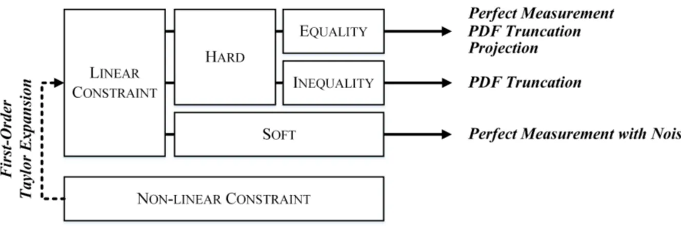
2.3 State Constraints . . . . 19

2.3.1 Hard Constraints . . . . 20

2.3.2 Soft Constraints . . . . 23

2.3.3 Non-linear Constraints . . . . 23

3 Methodological Contributions 27 3.1 Versatile Recursive State-space Filter . . . . 27

3.2 Kalman Filtering with State Constraints for Gauss-Helmert Models . . . . 28

3.2.1 Implicit Pseudo Observations . . . . 30

3.2.2 Constrained Objective Function . . . . 31

3.2.3 Improvement of Implicit Contradictions . . . . 32

3.3 Recursive Gauss-Helmert Model . . . . 34

3.4 Example of Application . . . . 35

3.4.1 Monte-Carlo Simulation and Consistency . . . . 38

3.4.2 Results . . . . 39

3.4.3 Conclusions . . . . 49

4 Kinematic Multi-sensor Systems and Their Efficient Calibration 51 4.1 Kinematic Multi-sensor Systems . . . . 51

4.2 Calibration of Laser Scanner-based Multi-sensor Systems . . . . 53

4.2.1 Motivation . . . . 53

4.2.2 Experimental Setup . . . . 55

4.2.3 Classical Methods . . . . 56

4.2.4 Novel Recursive Calibration Approach . . . . 60

4.2.5 Comparison and Discussion . . . . 61

5.2 Experimental Setup . . . . 72

5.2.1 Kinematic Laser Scanner-based Multi-sensor Systems . . . . 72

5.2.2 Scenarios and Measuring Process . . . . 74

5.2.3 Additional Object Space Information . . . . 78

5.3 State of the Art Methods . . . . 80

5.4 Novel Information-based Georeferencing Approach . . . . 83

5.4.1 Basic Idea . . . . 83

5.4.2 Transformation of the Laser Scanner Observations . . . . 85

5.4.3 Assignment of the Laser Scanner Observations . . . . 85

5.4.4 Application of the Versatile Recursive State-space Filter . . . . 88

5.5 Comparison and Discussion . . . . 92

5.5.1 Mapping Within an Inner Courtyard . . . . 94

5.5.2 Georeferencing of an Autonomous Vehicle Within an Urban Canyon . . . . . 96

5.5.3 Conclusions . . . . 102

6 Conclusions 105 6.1 Summary . . . . 105

6.2 Outlook . . . . 107

A Appendix 109 A.1 Pseudocode of the Versatile Recursive State-space Filter . . . . 109

A.2 Analysis for the Selection of a Suitable Measurement and Process Noise . . . . 110

Bibliography 113

Acknowledgments 121

Curriculum Vitae 123

2.1 Flowchart of the explicit IEKF . . . . 16

2.2 Flowchart of the implicit IEKF . . . . 19

2.3 Flowchart of the explicit IEKF with PMs . . . . 20

2.4 Impact of selecting the weight matrix in the PRO method . . . . 21

2.5 Flowchart of the explicit IEKF using the PRO method . . . . 22

2.6 Basic principle of the PDF truncation method . . . . 22

2.7 Flowchart of the explicit IEKF using the PDF truncation method . . . . 23

2.8 Flowchart of the explicit IEKF with SCs . . . . 24

2.9 Linearisation errors in case of non-linear state constraints . . . . 24

2.10 Overview of different methods for considering state constraints . . . . 25

3.1 Schematic overview and flow diagram of the versatile recursive state-space filter . . . 29

3.2 Flowchart of the implicit IEKF with PMs or SCs . . . . 30

3.3 Flowchart of the implicit IEKF with a COF . . . . 32

3.4 Simplified representation of iterative loops for improved linearisation and compliance with near-zero contradictions and state constraint equations . . . . 33

3.5 Flowchart of the implicit IEKF with PRO method and contradiction loop . . . . 33

3.6 Flowchart of the implicit IEKF with PDF truncation method and contradiction loop . 34 3.7 Schematic representation of an ellipse . . . . 36

3.8 Mean of the RMSE and the related confidence intervals . . . . 41

3.9 Temporal progression of the mean RMSE and related confidence intervals without con- sideration of constraints . . . . 42

3.10 Temporal progression of the mean RMSE and related confidence intervals with considera- tion of constraints . . . . 42

3.11 Standard deviations of the semi-major axis and the semi-minor axis . . . . 43

3.12 NEES for different recursive approaches . . . . 43

3.13 Mean of the maximum contradictions within each epoch . . . . 44

3.14 Mean of the RMSE with regard to biased eccentricity . . . . 45

3.15 Effect of wrong prior information when using SCs . . . . 46

3.16 Effect of wrong prior information when using PDF truncation . . . . 47

3.17 Mean RMSE for both semi-axes depending on measurement noise for soft and inequality constraints . . . . 48

3.18 Mean RMSE for various measurement noises when using SCs and wrong prior informa- tion . . . . 48

3.19 Mean RMSE for various factors when using inequality constraints and wrong prior infor- mation . . . . 49

4.1 Exemplary MSS on car roof with several sensors fixed to each other on a platform . . 52

4.2 Strongly simplified process chain of a kinematic MSS with its elementary tasks . . . 54

4.3 Laser scanner-based MSS with sensors and schematic representation of the MSS with related coordinate systems . . . . 55

4.4 Visualisation of the laser scanner-based MSS during its calibration . . . . 56

4.5 The basic calibration procedure with regard to the measurement execution and the subse-

quent adjustment strategies . . . . 57

4.6 Schematic representation of the transformations to be applied during the calibration . 59 4.7 Sequence of one single run during MC simulation . . . . 64

4.8 Histograms of the estimated translations in Z-direction . . . . 66

4.9 Sequence of one single run during 10-fold cross-validation . . . . 67

4.10 Results of the k-fold cross-validation with k = 10 . . . . 68

5.1 Overview of the two kinematic laser scanner-based MSSs . . . . 73

5.2 Map-based representation of the two application scenarios . . . . 74

5.3 Images of the measured area in a spacious inner courtyard . . . . 75

5.4 Images of the measured area in an urban canyon . . . . 76

5.5 Measurement configuration to provide a highly accurate reference trajectory . . . . . 77

5.6 Part of the DTM for the different measurement areas . . . . 79

5.7 Illustration of the three-dimensional building model with LoD-2 . . . . 79

5.8 Simplified overview of three typical environments in which a kinematic MSS operates 84 5.9 Simplified process of the information-based approach for georeferencing a laser scanner- based MSS in urban areas by means of a flowchart . . . . 84

5.10 Schematic illustration of the general principle for assigning the laser scanner point cloud to the building model . . . . 86

5.11 Process of assigning laser scanner observations . . . . 88

5.12 Representation of the estimated trajectories with respect to the building model . . . . 92

5.13 Transformed point clouds for the scenario in the inner courtyard based on the estimated poses . . . . 95

5.14 Time variation of the estimated pose and their estimated standard deviations . . . . . 96

5.15 Time variation of different pose and position information . . . . 98

5.16 Transformed point clouds for the scenario in the urban canyon based on the estimated poses . . . . 99

5.17 Visualisation of the RMSE over all epochs by considering the original Riegl pose as addi- tional information as well as the assigned object space information . . . . 100

5.18 Visualisation of the RMSE over all epochs by considering the artificial pose as additional information as well as the assigned object space information . . . . 101

A.1 Mean RMSE for various factors when using recursive GHM without constraints . . . 110

A.2 Mean RMSE for various factors when using recursive GHM without constraints . . . 111

3.1 Compliance and non-compliance with the measurement equation and constraint equation

in the case of implicit relationships . . . . 30

3.2 Overview of the investigated methods with regard to their respective properties . . . 37

3.3 Mean relative run times with related standard deviations . . . . 39

3.4 Mean of the estimated semi-major axis and semi-minor axis together with corresponding standard deviations . . . . 40

3.5 Classification of the methods presented according to possible advantages, disadvantages or neutrality . . . . 50

4.1 Compilation of possible sensor types for kinematic MSSs . . . . 53

4.2 Compilation of possible platform types for kinematic MSSs . . . . 53

4.3 Estimated calibration parameters if all available observations are used . . . . 63

4.4 Estimated standard deviations if all available observations are used . . . . 63

4.5 Necessary absolute and relative run times by using 7000 individual 3D point observa- tions . . . . 64

4.6 Median of the absolute and relative run times with related standard deviations of the MC simulation . . . . 65

4.7 Median of the estimated calibration parameters . . . . 65

4.8 Median of the estimated standard deviations of the calibration parameters . . . . 65

5.1 Summary of the specific circumstances and key information for the two scenarios . . 93

5.2 Overview of the standard deviations used for each of the two scenarios . . . . 94

BIM Building Information Modeling . . . 1

BLUE Best Linear Unbiased Estimate . . . 6

C-GHM Constrained Gauss-Helmert Model . . . 11

C-GMM Constrained Gauss-Markov Model . . . 9

CCR Corner Cube Reflector . . . 76

COF Constrained Objective Function . . . 29

CPU Central Processing Unit . . . 49

DHHN2016 Deutsches Haupthöhennetz 2016 . . . 78

DMI Distance Measurement Indicator . . . 73

DoF Degrees of Freedom . . . 8

DSKF Dual State Kalman Filter . . . 107

DTM Digital Terrain Model . . . 78

EKF Extended Kalman Filter . . . 13

EnKF Ensemble Kalman Filter . . . 13

ETRS89 European Terrestrial Reference System 1989 . . . 74

GHM Gauss-Helmert Model . . . 3

GMM Gauss-Markov Model . . . 6

GNSS Global Navigation Satellite System . . . 1

GPS Global Positioning System . . . 52

GPU Graphics Processing Unit . . . 2

ICP Iterative Closest Point . . . 81

IEKF Iterated Extended Kalman Filter . . . 15

IMU Inertial Measurement Unit . . . 1

KF Kalman Filter . . . 13

LKF Linear Kalman Filter . . . 97

LoD Level of Detail . . . 78

LS Least-Squares . . . 5

MAP Maximum a Posteriori Probability . . . 14

MC Monte-Carlo . . . 27

MHE Moving Horizon Estimation . . . 24

MMS Mobile Mapping System . . . 1

MMSE Minimum Mean Square Error . . . 14

MPE Maximum Permissible Error . . . 54

MSS Multi-Sensor System . . . 1

NEES Normalised (State) Estimation Error Squared . . . 38

NLOS Non-Light-Of-Sight . . . 72

PCS Platform Coordinate System . . . 52

PDF Probability Density Function . . . 14

PF Particle Filter . . . 13

PM Perfect Measurement . . . 20

PPS Pulse Per Second . . . 52

PRO Projection . . . 21

RANSAC Random Sample Consensus . . . 87

RMSE Root-Mean-Square Error . . . 40

RTG Research Training Group . . . 3

SC Soft Constraint . . . 19

SCKF Smoothly Constrained Kalman Filter . . . 24

SLAM Simultaneous Localisation and Mapping . . . 81

SOCS Sensor Own Coordinate System . . . 54

SVM Support Vector Machine . . . 82

UAV Unmanned Aerial Vehicle . . . 1

UKF Unscented Kalman Filter . . . 13

UTM Universal Transverse Mercator . . . 74

V2I Vehicle-to-Infrastructure . . . 82

VCM Variance-Covariance Matrix . . . 5

WCS World Coordinate System . . . 56

1 Introduction

1.1 Motivation

The use of domestic robots (e.g. robotic vacuum cleaners) has increased steadily in recent years. As a result, it has become a widespread routine that such mainly autonomously acting systems are moving in the immediate environment of humans (Bogue, 2017). The risk potential for these small robots to in- jure humans is, in this context, quite low. However, the situation will be completely different, if in the upcoming years more and more fully autonomous cars will be involved in public road traffic. Already today, local public transport buses and taxis operate autonomously in defined areas, with a growing trend (Fagnant and Kockelman, 2015; Mallozzi et al., 2019; Boudette, 2019). At present, the presence of a trained operator is still mandatory to ensure safety. Unexpected collisions can have serious consequences in this context, which must be prevented. For this reason, vehicles are already equipped with a variety of different sensors. In addition to vehicle-specific sensors, these are mainly those that are used for posi- tioning and orientation of the vehicle to its environment (e.g. Global Navigation Satellite System (GNSS) antennas or Inertial Measurement Units (IMUs)). Furthermore, there exist sensors that are increasingly used for environmental perception, such as laser scanners and cameras. In combination, they ensure the integrity

of the vehicle. The accurate, precise, reliable and complete pose

estimation of such a system is of great importance. Its exact determination must be known continuously at all points in time. This must be ensured independently of the environment.

However, these requirements are of great importance not only for autonomous vehicles. In general, these demands can also be applied to any kinematic Multi-Sensor System (MSS). After all, a modern vehicle with all its sensors is nothing else than such a kinematic MSS. Therefore, accurate information about the current position and orientation is not only necessary to ensure the integrity of a vehicle, but it is also essential for other purposes. In this context, it can generally also refer to the georeferencing of an MSS with respect to a superordinate coordinate system. For example, accurate and precise pose estimation is also indispensable when using Mobile Mapping Systems (MMSs) on the ground and in the air. These MMSs are mobile platforms containing several of the above-mentioned sensors in order to acquire spatial data of the environment (Wang et al., 2019). Such systems usually do not operate autonomously, but even in case of, i.e. an Unmanned Aerial Vehicle (UAV), their pose to a fixed coordinate system must be precisely known at all times (Colomina and Molina, 2014). Only under these conditions, it is possible to derive highly accurate maps and three-dimensional models of the reality from the acquired data (Glennie, 2007).

This, in turn, is the basis for obtaining, for example, an up-to-date Building Information Modeling (BIM) system (Borrmann et al., 2018) or 3D city models (Vosselman and Dijkman, 2001).

Although numerous approaches and methods already exist, independence with respect to the environment is still a major challenge. Urban areas, in particular, cause difficulties. So-called urban canyons lead to the fact that the otherwise frequently used pose information based on GNSS and IMU observations is

1Integrity, in this context, means that the complete, safe and accurate operability of the vehicle within certain predefined thresh- olds can be guaranteed at all times, and that information is provided in a timely manner if these thresholds are exceeded (Hegarty et al., 2017).

2combination of position and orientation in the relevant dimension

often too inaccurate (Zhu et al., 2018). Shadowing as well as multipath and drift effects are the reasons for this. Such unreliable georeferencing is risky, especially in highly frequented urban environments. This circumstance has led to the fact that other sensors for georeferencing, such as laser scanners and cam- eras, as well as additional map information, are already being considered more intensively in the systems mentioned. Thus, the acquired data cannot only be used to map the environment but also to actively contribute to the improvement of georeferencing. However, this leads simultaneously to new challenges.

Especially the increased use of laser scanners in such kinematic MSSs leads to an enormous increase in the amount of data collected. Besides, automotive laser scanners (such as solid-state scanners), for ex- ample, have recently become less expensive, which makes them even more suitable for more frequent use in cars for the future (Randall, 2019). There are already multiple automotive laser scanners available that have a small and lightweight design and a remarkable level of accuracy (Velodyne LiDAR, 2018b;

Ibeo Automotive Systems, 2020; Robosense, 2020). At the same time, the resolution, range and density of these three-dimensional sensors are increasing. The availability of at least 500 000 points per second is already common. Slightly larger sensors than such automotive laser scanners already capture about 2.2 million points per second (Velodyne LiDAR, 2018a). For this reason, the terminology of big data is quite appropriate in this context. Big data requires the need for efficient algorithms to realise potentially real-time capable systems. To process these vast amounts of point cloud data at all, usually, only a random subset of the total collected data is currently used (Elseberg et al., 2013b). Although there are approaches that perform spatial or temporal subsampling, there is no specific assessment of the individual observed quantities with regard to their contribution to an improved estimation. Thus, a more structured reduction of the entire data set is achieved, but important observations might be lost. Since this identification of relevant observations is quite challenging, depending on the application, it is advisable to use as much information as possible. Batch processing, where the data is used within an overall adjustment, is often applied for this purpose, but reaches its limitations with such increasing amounts of 3D points. Although such batch methods provide excellent results, they usually have to be performed in post-processing on powerful com- puters. Otherwise, enormous mobile computing power is required or, for example, the use of Graphics Processing Units (GPUs). However, this is in contradiction to the demands for online approaches, such as those needed for autonomous driving. Current applications of this kind require recursive approaches.

Especially suitable for such tasks is the use of recursive state-space filtering. This methodology covers decades of development and deals with the estimation of arbitrary and not directly measurable states, by the fusion of arbitrary observation data via a suitable mathematical model (Kalman, 1960). Applications of such filters are extensive. However, these are primarily based on explicit

mathematical relationships between the observations and the parameters to be estimated. This mathematical limitation is in contrast to a multitude of issues in various fields of expertise (Heuel, 2001; Perwass et al., 2005), and especially in geodesy (Steffen and Beder, 2007; Dang, 2007; Ning et al., 2017). Often, when dealing with geometri- cal issues, mathematically implicit

relationships occur. Although there are approaches but they are rare.

This becomes evident, for example, from the fact that the use of constraints regarding the state param- eters in connection with implicit relationships has not yet been investigated. However, the presence of appropriate additional information when using constraints is always recommended and generally has a beneficial impact on the estimation results (Simon, 2010). For example, the integration of various (geo- metric) constraints regarding the previously mentioned challenging urban setting for autonomous driving might be useful. In addition, there is still a need to develop and assess these methods with regard to compliance with integrity aspects (Wörner et al., 2016; Reid et al., 2019). Therefore, possible solutions should consider the inclusion of new independent and complementary sources of information. This will further improve redundancy, and any loss of integrity can be identified and reported in a timely manner.

In summary, due to the availability of inexpensive modern sensor technologies, the amount of data for various current topics is constantly increasing. Consequently, there is a demand to develop new recursive methods for the reliable georeferencing of kinematic MSSs in challenging urban environments. This allows ensuring the integrity of, e.g. autonomous vehicles or to accurately map environments when using MMSs. Solutions are based on applications from the field of recursive state-space filtering in combination with appropriate constraints and additional information from object space.

3The observations result directly from the parameters under consideration of a functional relationship

4The observations and parameters cannot be separated from each other to either side of the equation.

1.2 Objective and Outline

The main focus of this thesis is on the development of a versatile Kalman filter. This filter should consider non-linear explicit and implicit mathematical relationships between available observations and requested state parameters. In addition, existing methods for the consideration of arbitrary non-linear state con- straints have to be applied and validated for the implicit relationships. The main focus here lies on the distinction between hard and soft constraints, and their application to prior information which is affected by a specific degree of uncertainty. It is also necessary to analyse the impact of wrong prior information with regard to the different methods for taking constraints into account. The application of the methodol- ogy in this thesis is directly related to kinematic MSSs and associated tasks, like their efficient calibration and georeferencing. In particular, this addresses current challenges in complex urban environments, as well as the development of methods for georeferencing with integrity aspects even under such difficult conditions. For this purpose, independent and complementary sources of information should be used, providing at least long-term support. However, basic applicability to any other issues should also be pos- sible. For this reason, it is also necessary to investigate the extent to which the newly developed methods within this thesis perform with vast amounts of data compared to the existing approaches. This is directly related to current and future big data applications. According to these objectives, this thesis is structured as follows.

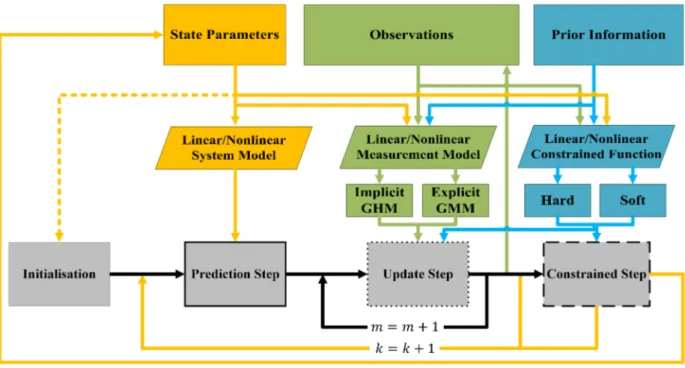
Chapter 2 gives an overview of the methods and models applied in this thesis. Firstly, this includes the fundamentals of parameter estimation and associated models. Secondly, the idea of recursive state- space filtering is presented. The corresponding methodology is provided for both explicit and implicit relationships. Thirdly, a comprehensive overview of different possibilities for the consideration of linear and non-linear state constraints is given.

The own methodological contributions of this thesis are presented in chapter 3. This includes the intro- duction of the versatile recursive state-space filter and mainly the possibilities to consider different state constraints in the context of implicit measurement equations. Furthermore, a realisation of a recursive Gauss-Helmert Model (GHM) is presented from these studies. Also, a geometric application example is presented, which serves as the validation base for the described methods.

Chapter 4 contains a detailed application of the proposed methods concerning the calibration of a kine- matic MSS. A general definition of such a system is given at the beginning, and the primary tasks involved are described. This is followed by the motivation and description of the specific calibration task. The re- sults based on the new methods are presented and discussed concerning existing standard approaches.

A second application related to the georeferencing of kinematic MSSs is described in chapter 5. In ad- dition to a motivation and a description of the experimental setup used, current methods of solving the problem are discussed together with their weaknesses. Subsequently, the newly developed approach and the respective results are presented and evaluated.

The thesis concludes with a summary of the most relevant results and findings in chapter 6. At last, an outlook is given in which remaining questions are formulated, and ideas for further research are presented.

The new methods developed in this thesis, the measurement data acquired and the findings obtained are

directly related to the Research Training Group (RTG) i.c.sens 2159, funded by the Deutsche Forschungs-

gemeinschaft (DFG, German Research Foundation). Furthermore, parts of the computations were per-

formed by the compute cluster, which is funded by the Leibniz Universität Hannover, the Lower Saxony

Ministry of Science and Culture (MWK) and DFG.

2 Fundamentals of Recursive State-space Filtering

This chapter is dedicated to the basic principles of recursive state-space filtering. As part of the parameter estimation in section 2.1, two well-known adjustment models for overdetermined equation systems are generally introduced. These models are then extended by the consideration of constraints. Based on this, the differences to the recursive state-space filtering in section 2.2 are presented. These filters are generally applied to non-linear relationships, which must be exclusively explicit in a first method and implicit in a further method. Subsequently, section 2.3 gives a detailed overview of the various possibilities for considering state constraints in Kalman filtering.

2.1 Parameter Estimation

Adjustment theory provides a fundamental structure for solving overdetermined systems of equations.

Such problems are omnipresent in many scientific communities. During a measurement process, arbitrary types of observations l

are carried out to determine the unknown parameters x

. Corresponding parameters and observations can be arbitrarily suitable physical or mathematical quantities (e.g., coordinates, angles, distances). The relationship between these observations and parameters can be formulated by any suitable mathematical real-valued functions

h (·), depending on the respective application. This becomes reason- able if the unknown parameters are not directly observable (e.g., coordinates of a new point by observed distances and angles from known points). Furthermore, a set of overdetermined equation systems can increase reliability (e.g., detection of outliers) and improve quality measures (e.g., accuracy, precision).

By contrast, overdetermined equation systems can have multiple solutions. For this reason, the optimal solution of such an equation system must be found by parameter estimation.

Different adjustment models can realise such an estimation. The correct choice of the model depends on the independent functional relationships between the observations available and the parameters requested.

A careful derivation of such functions by physical or mathematical laws is essential. However, strictly speaking, functional relations are only valid for the true observations ˜ l

and parameters ˜ x

. To overcome inconsistencies, unknown expected values E (·) are included when using the real values. Furthermore, residuals are introduced to use the real observations and parameters to the respective model (Niemeier, 2008, pp. 120 ff.). This procedure will lead to the best estimates of the values requested.

A stochastic model is used to account for the random behaviour of the observations. In a simplified approach, independent and identically distributed random variables are usually applied. It is assumed that the observed values result from additive deviations — which are random — from the true values. The uncertain observations are therefore modelled by any distribution, e.g. by the Gaussian distribution. An expected value and a Variance-Covariance Matrix (VCM) can give the distribution. This stochastic model will influence the estimation of the unknown parameters as well as their quality measures.

Furthermore, the respective adjustment model is applied with an arbitrary estimator. The most common estimator is Least-Squares (LS). Underlying concept of the optimisation criterion is to minimise the sum

1Also referred to asfunctional model

of the squared residuals between real observations l

and their related expected values E (l

) = h

(x) by the unknown parameters x (Koch, 1999, pp. 152). If the functional model h (·) is linear, the estimation is referred to as Best Linear Unbiased Estimate (BLUE) in the context of the optimality properties. The strict solution of the LS estimator is independent from the underlying distribution of the observations (Förstner and Wrobel, 2016, pp. 80 ff.). Also other (robust) estimators (e.g. Huber, Hampel) can be applied, which are based on maximum likelihood methods. Nevertheless, only the LS estimator is used in the following.

The general case of adjustment, also known as GHM, forms the basis for such adjustment models. The special case, also known as Gauss-Markov Model (GMM) and the transformation of a GHM into an equivalent GMM are presented subsequently. Such standard methods are commonly used in the geodetic community and are described in detail by (Koch, 1999; Lenzmann and Lenzmann, 2004; Jäger et al., 2005;

Wichmann, 2007; Niemeier, 2008). Furthermore, consideration of additional constraints to the requested parameters is given at least for the GMM by the authors mentioned. However, constraints in the sense of a GHM are rather an exception and are mentioned by only a few authors, such as (Rietdorf, 2005;

Lösler and Nitschke, 2010; Steffen, 2013; Heiker, 2013; Roese-Koerner, 2015).

There are two basic possibilities for realisation of LS adjustment. The particular preference depends on the existing application. Measurements can be carried out as a whole, which will result in a post- processing approach for all available observations acquired. This will be referred to as overall adjustment or batch approach. In contrast to such a batch approach, new observations can be considered epochwise as soon as they are acquired. This will result in a recursive parameter estimation

approach. This means the parameters requested are updated step-by-step by latest observations available. However, recursive parameter estimation for a GHM does not exist at all.

In general, it is assumed to receive only a well-posed normal equation system to obtain a unique inverse of a regular matrix. Singular entities, e.g., due to datum defects or linear dependencies, are not considered and would require additional special attention.

It should be noted that the different adjustment models partly use the same denominations for the non- linear functions as well as individual vectors and matrices. This multiple use is intended to ensure clarity.

However, — if not mentioned otherwise — new variables can be assumed when a new adjustment model is introduced.

2.1.1 Gauss-Markov Model

Unconstrained Gauss-Markov Model

The GMM, also referred to as adjustment of observations, represent an explicit relation between stochastic observations and unknown deterministic parameters. In general, the non-linear GMM is defined by the n × 1 observation vector l and the u × 1 parameter vector x as

E (l) = h (x) , (2.1)

or without expected values of the observations and more detailed

l

+ v

= h

(x

, x

, . . . , x

) . (2.2)

The residuals within the vector v are assumed to be Gaussian with expected value E (v) = 0

v ∼ N (0, Σ

) with Σ

= σ

· Q

= σ

· P

, (2.3) where Σ

is the known positive-definite VCM of the observations, Q

the related cofactor matrix, σ

the a priori variance factor and P the weight matrix. Altogether they describe the weighting of the observations among each other and are referred to as stochastic model. A linear functional model h (·) is required for

2Also referred to assequential parameter estimation(Niemeier, 2008, pp. 314 ff.)

the adjustment. Linearisation of Equation (2.2) can be performed for non-linear models by Taylor series expansion up to the linear segment, which leads to the matrix form

l + v = h (x

)

| {z }

l0

+ A · (x − x

)

| {z }

∆x

with A = ∇

h (x)

(2.4a)

= l

+ A · ∆x with ∆l = l − l

. (2.4b)

The design matrix A is assumed to be of full rank and the partial derivatives are evaluated at the initial parameters x

. It should be noted that in the following process only the parameter vector x is used instead of the reduced parameter vector ∆x. Therefore, the necessary updating must still be taken into account.

The same applies to the reduced observation vector ∆l and the initial observations l

. In addition, the estimated values of the individual quantities are only given from the level of the normal equations. Up to this stage, the unknown true values are given. Regardless of this, the linearisation should also apply to the estimated values. To obtain an optimal estimation of the parameters, the residuals of the objective function L

(x) are minimised according to LS estimation (cf. section 2.1). The Gauss-Newton method is used for this purpose, hence

L

(x) = v

· P · v (2.5a)

= (A · x − l)

· P · (A · x − l) (2.5b)

= x

· A

· P · A · x − 2 · x

· A

· P · l + l

· P · l → min. (2.5c) This is done by setting the partial derivative of the objective function with respect to the optimisation variable x equal to zero (Wichmann, 2007, pp. 106)

∇

L

(x) = 2 · A

· P · A · x − 2 · A

· P · l =

0. (2.6) This leads to the optimal estimation of the parameters by using LS adjustment (Koch, 1999, pp. 158)

ˆ x =

A

· P · A

| {z }

NGMM

−1

· A

· P · l, (2.7)

where N

is the normal equation matrix. The estimated residuals ˆ v can be obtained by

ˆ v = A · ˆ x − l (2.8)

to receive the adjusted observations ˆ l

ˆ l = l + ˆ v. (2.9)

The cofactor matrix Q

with the co-/variances of the estimated parameters ˆ x can be obtained by the inverse of the regular normal equation matrix N

Q

= N

=

A

· P · A

. (2.10)

Taking into account the a posteriori variance factor σ ˆ

= ˆ v

· P · ˆ v

n − u , (2.11)

the estimated VCM Σ ˆ

for the estimated parameters results in

Σ ˆ

= ˆ σ

· Q

. (2.12)

In addition, the following also applies

Σ

= σ

· Q

, (2.13)

where the VCM Σ

refers to the a priori variance factor. This VCM is of interest if the Degrees of Freedom (DoF) of the adjustment task are low or if the estimation cannot be trusted for other reasons.

Strict recommendations on when to prefer which VCM do not exist. This depends on the specific task and the present (measurement) configuration. In the context of this thesis appropriate conditions are assumed.

For this reason, Σ

will not be given in the following.

Constrained Gauss-Markov Model

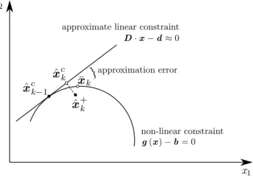
The parameters x might be restricted by s independent non-linear equality constraints

g (x) = b, (2.14)

with independent real-valued non-linear functional relations g (·) and the related constant s × 1 vector b.

Similar to the non-linear functional model in Equation (2.2), the non-linear constraint function g (·) needs to be linearised by Taylor expansion. A truncation of the Taylor expansion after the linear term leads to the following substitution

C · x = d with C = ∇

g (x)

, (2.15a)

d = b − g (x

) + C · x

, (2.15b)

where C is the u × s matrix of equality constraints and d is the related constant s × 1 vector. Such an extension by constraints can be reasonable in case of suitable prior information regarding mathematical relationships between specific parameters. A common example of using equality constraints is to ensure a normalised normal vector of a plane. To apply such additional information, the objective function in Equation (2.5c) must be extended

L

(x, λ) = L

(x) + 2 · λ

(C · x − d) → min (2.16a)

= x

· A

· P · A · x − 2 · x

· A

· P · l + l

· P · l

+ 2 · λ

(C · x − d) → min, (2.16b)

with the s×1 vector λ of Lagrangian multipliers. The solution is again achieved through the related partial derivatives of the Lagrangian according to the Gauss-Newton method. These derivatives are set equal to zero with respect to x and λ (Koch, 1999, pp. 170 ff.)

∇

L

(x, λ) = 2 · A

· P · A · x − 2 · A

· P · l + 2 · C

· λ =

0, (2.17)

∇

L

(x, λ) = 2 · (C · x − d) =

0. (2.18)

On this basis, Equation (2.7) need to be extended into a block structure A

· P · A C

C 0

| {z }

N_C-GMM

"

ˆ x λ ˆ

#

=

A

· P · l d

, (2.19)

where N

is the extended normal equation matrix. As Roese-Koerner (2015, pp. 16) mentioned,

Lagrange multipliers do not have a physical unit and often a multiple is used to ensure convenient equa-

tions. The linear system of Equation (2.19) has an unique solution if the bordered normal equation matrix

N

is regular (N

need to be of full rank) (Wichmann, 2007, pp. 113). The cofactor matrix Q

with the co-/variances of the estimated parameters ˆ x can be obtained by the inverse of the normal equation matrix N

.

The extension with regard to the VCM Σ ˆ

results from Equation (2.12), whereby σ ˆ

results under con- sideration of the s constraints as follows

σ ˆ

= ˆ v

· P · ˆ v

s + n − u . (2.20)

Finally, it should be noted that within this Constrained Gauss-Markov Model (C-GMM) only equality and no inequality constraints can be taken into account.

2.1.2 Gauss-Helmert Model

Unconstrained Gauss-Helmert Model

The general case of adjustment becomes applicable, as soon as n × 1 stochastic observations and u × 1 unknown deterministic parameters are strictly interconnected by an arbitrary real-valued function h (·) . Such a non-linear implicit relation can be formulated by equality constraints

h ( E (l) , x) =

0, (2.21)

or by using residuals instead of the expected values of the observations

h

(l

+ v

, l

+ v

, . . . , l

+ v

, x

, x

, . . . , x

) = 0,

(2.22) To obtain a linear functional model approximate values l

and x

to both observations and parameters need to be selected carefully for Taylor series expansion (Lenzmann and Lenzmann, 2004). The following applies

h (l + v, x) = h (l

+ ∆l + v, x

+ ∆x) with ∆l = l − l

(2.23a)

≈ h (l, x)

| {z }

w0

+ ∇

h (l, x)

| {z }

B

· (∆l + v) + ∇

h (l, x)

| {z }

A

·∆x (2.23b)

= w

+ B · (∆l + v) + A · ∆x (2.23c)

= w

+ B · ∆l

| {z }

w

+ B · v + A · ∆x (2.23d)

= B · v + A · ∆x + w =

0, (2.23e)

where B is the q × n condition matrix with partial derivatives of the q condition equations with re- spect to the observation vector l, and w refers to the q × 1 vector of contradictions. According to Lenzmann and Lenzmann (2004), note that the partial derivatives are evaluated at the location

of

l = l

+ v, (2.24)

x = x

+ ∆x, (2.25)

where the residuals v and the reduced parameter vector ∆x will continuously change during the estimation.

To obtain an estimate for l, v, x and ∆l minimising of the objective function L

(v, ∆x, λ) with respect to LS estimation (cf. section 2.1) can be performed by Lagrangian multipliers

L

(v, ∆x, λ) = v

· P · v − 2 · λ

(B · v + A · ∆x + w) → min. (2.26)

3Also referred to asdevelopment point

Setting the related partial derivatives with respect to v, ∆x and λ equal to zero

∇

L

(v, ∆x, λ) = 2 · P · v − 2 · B

· λ =

0 ⇔ v = P

B

· λ, (2.27)

∇

L

(v, ∆x, λ) = −2 · A

· λ =

0 ⇔ A

· λ = 0, (2.28)

∇

L

(v, ∆x, λ) = −2 · (B · v + A · ∆x + w) =

0 ⇔ B · v + A · ∆x + w = 0, (2.29) leads to the solution of the restricted minimisation problem by the linear normal equation system in block structure

"

B · P

· B

A

A

0

#

| {z }

NGHM

"

λ ˆ

∆ˆ x

#

= −w

0

. (2.30)

Depending on the selection of reasonable approximate values for l

and x

, several iterations for repeated linearisation are required to obtain accurate estimates for the unknown parameters. Assuming that the inverse of N

exist, the estimates for each iteration are

Q

= B · P

· B

, (2.31)

ˆ k = Q

I − A ·

A

· Q

· A

· A

· Q

· (−w) , (2.32)

ˆ v = Q

· B

· ˆ k, (2.33)

ˆ l = l

+ ˆ v, (2.34)

as well as

∆ˆ x =

A

· Q

· A

· A

· Q

· (−w) , (2.35a)

ˆ x = x

+ ∆ˆ x. (2.35b)

The cofactor matrix Q

with the co-/variances of the estimated parameters ˆ x can be derived either by inverting the entire regular normal equation matrix N

N

=

"

Q

Q

Q

x

−Q

#

, (2.36)

or by applying the law of error propagation

to the estimated parameters in Equation (2.35a), which leads to

Q

=

A

· Q

· A

. (2.37)

Also here the extension results to the a posteriori VCM Σ ˆ

according to Equations (2.11) and (2.12).

Again, the a priori VCM Σ

can be obtained according to Equation (2.13), whereby the same applies with regard to its use as for GMM.

Constrained Gauss-Helmert Model

Similar to the C-GMM, the parameters x of the GHM might be also restricted by s independent non-linear equality constraints

g (x) = b, (2.38)

4Also referred to aspropagation of uncertainty

which can be transformed according to Equation (2.15) into linear constraints

C · x = d. (2.39)

According to (Roese-Koerner, 2015, pp. 19 ff.) the parameter vector x needs to be divided into the approximation value x

and the reduced parameter vector ∆x, which leads to

C (x

+ ∆x) = d

(2.40a)

C · ∆x = d

− C · x

=: d. (2.40b)

The consideration of suitable prior information for a Constrained Gauss-Helmert Model (C-GHM) makes it necessary to extend the objective function in Equation (2.26) to

L

( v, ∆ x, λ

, λ

) = L

( v, ∆ x, λ) − 2 · λ

( C · ∆ x − d ) → min (2.41a)

= v

· P · v − 2 · λ

(B · v + A · ∆x + w)

− 2 · λ

(C · ∆x − d) → min. (2.41b)

As in the unconstrained GHM, the related partial derivatives with respect to v, ∆ x, λ

and λ

of the Lagrangian are set equal to zero

∇

L

(v, ∆x, λ

, λ

) = 2 · P · v − 2 · B

· λ

=

0

⇔ v = P

B

· λ

,

(2.42)

∇

L

(v, ∆x, λ

, λ

) = −2 · A

· λ

− 2 · C

· λ

= 0

⇔ A

· λ

+ C

· λ

= 0, (2.43)

∇

L

(v, ∆x, λ

, λ

) = −2 · (B · v + A · ∆x + w) =

0

⇔ B · v + A · ∆x + w = 0, (2.44)

∇

L

(v, ∆x, λ

, λ

) = − (C · ∆x − d) =

0

⇔ C · ∆x = d, (2.45)

leads to the solution of the constrained minimisation problem by the linear normal equation system in block structure







B · P

· B

A 0 A

0 C

0 C 0







| {z }

N_C-GHM







λ ˆ

∆ˆ x λ ˆ







=





−w 0 d





. (2.46)

Again, several iterations for repeated linearisation are required and the cofactor matrix Q

can be derived by inverting the regular normal equation matrix N

N

=







Q

Q

Q

Q

1ˆx

−Q

Q

Q

k1ˆk2

Q

xˆk2

−Q

2ˆk2







. (2.47)

By substitution and transformation of Equations (2.42) and (2.43) the corresponding residuals read

ˆ v = −P

· B

B · P

· B

· (A · ∆ˆ x + w) , (2.48)

with which the estimated VCM Σ ˆ

for the estimated parameters ˆ x can be obtained according to Equations

(2.12) and (2.20).