Eective One-Dimensional Models from Matrix Product States

from Matrix Product States

Masterarbeit

zur Erlangung des akademischen Grades Master of Science

vorgelegt von

Frederik Keim

geboren in Tettnang

Lehrstuhl für Theoretische Physik I Fakultät Physik

Technische Universität Dortmund

2012

Datum des Einreichens der Arbeit: 28. September 2012

product state formalism is introduced. It exploits tranlational invariance to to work di- rectly in the thermodynamic limit. The method is tested on the analytically solvable Ising model in a transverse magnetic eld. Results for ground state energy and dispersion are given as well as a way to nd a real space representation for the local creation operator.

From this, the one particle contribution to the spectral weight is calculated.

Kurzfassung

In dieser Arbeit wird eine variationelle Methode zur Ableitung eektiver eindimensionaler

Modelle vorgestellt, die auf dem Formalismus der Matrixproduktzustände basiert. Durch

Ausnutzung von Translationsinvaranz kann direkt im thermodynamische Limes gearbeitet

werden. Die Methode wird anhand des Ising Modells in einem transversalen Magnetfeld

getestet, das exakt lösbar ist. Es werden Ergebnisse für die Grundzustandsenergie und

die Einteilchen-Dispersion angegeben, sowie ein Weg den lokalen Erzeuger im Ortsraum

zu konstruieren. Damit wird der Einteilchen-Beitrag zum spektralen Gewicht berechnet.

Contents V

List of Figures VI

List of Tables VII

1 Introduction 1

1.1 Motivation . . . . 1

1.2 Existing methods . . . . 1

1.3 The approach . . . . 3

1.4 Structure of the thesis . . . . 3

2 Model and general approach 5 2.1 The transverse eld Ising model . . . . 5

2.2 Introduction to matrix product states . . . . 9

2.3 Eective models . . . 21

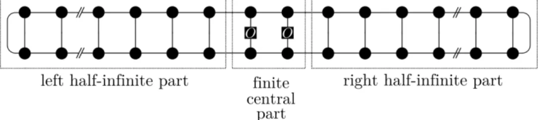
3 Ground state energy 23 3.1 Matrix product states for innite systems . . . 23

3.2 Variational ground state search . . . 30

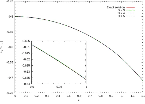
3.3 Results . . . 37

3.4 Existing methods . . . 38

4 Dispersion 39 4.1 Description of excitations . . . 39

4.2 Algorithm . . . 46

4.3 Results . . . 47

4.4 Existing methods . . . 51

5 Local creation operator and spectral weight 53 5.1 Local creation operator . . . 53

5.2 Spectral weight . . . 55

6 Conclusions and outlook 63 6.1 Summary of method . . . 63

6.2 Summary of results . . . 63

6.3 Outlook . . . 64

Bibliography 65

2.1 Construction of left-canonical MPS . . . 10

2.2 Graphical representation of local matrices A

. . . 12

2.3 Tensor network representation of local matrices A

at the edges and in the bulk of the chain. The matrcies at the edges are simply vectors and therefore have only one matrix index α

and α

respectively. Complex conjugates that arise in the description of bra-vectors are depicted with a downward pointing physical index. . . 12

2.4 Application of matrix product operator . . . 16

2.5 System buildup in numerical renormalization groups . . . 17

2.6 Superblock in standard DMRG . . . 18

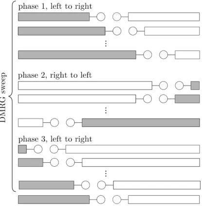
2.7 DMRG sweep . . . 20

3.1 Splitting scheme for innite systems . . . 23

3.2 Diagram for local MPO . . . 29

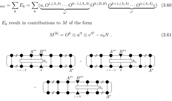
3.3 Central contributions to M matrix . . . 34

3.4 Ground state energy per lattice site E

/L . . . 37

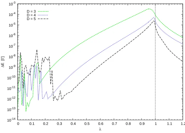
3.5 Deviation of ground state energy from exact result . . . 38

4.1 Results from naive dispersion approach . . . 41

4.2 Eigenvalues of the norm matrix N

. . . 43

4.3 Tensor network for norm element N

. . . 43

4.4 Representative contributions to the matrix element h

. . . 44

4.5 Dispersion for λ = 0.5 . . . 48

4.6 Dispersion for λ = 0.9 . . . 49

4.7 Dispersion for λ = 1.0 . . . 49

4.8 Excitation gap energy ∆ . . . 50

4.9 Deviation of ∆ from exact result . . . 50

5.1 Eigenvector v

of momentum space EVP . . . 54

5.2 Coecients v

of creation operator (linear) . . . 55

5.3 Coecients v

of creation operator (log.) . . . 56

5.4 Sepctral weight S

for λ = 0.5 . . . 58

5.5 Sepctral weight S

for λ = 0.9 . . . 58

5.6 Sepctral weight S

for λ = 0.999 . . . 59

5.7 Correlation length . . . 60

2.1 Examples on tensor network notation . . . 12

3.1 Local variation algorithm . . . 36

3.2 Extended ground state search algorithm . . . 36

4.1 Alorithm for calculating the energy dispersion . . . 46

4.2 Comparison of result quality for E

and ω

. . . 47

Introduction

1.1 Motivation

One of the main elds of research in quantum many body physics are systems of strongly correlated electrons. Sometimes, mostly for one-dimensional models, special properties of a given model allow for an analytical solution. However, the number of such models is small and in general one will have to resort to numerical calculations. The exponential growth of the Hilbert space dimension with the number of particles strongly limits the size of a system that can be analyzed by exact diagonalization.

There are various approaches to work around these limitations. Renormalization group methods try to concentrate the computational power of a classical computer on a fraction of the Hilbert space in which the physics takes place that one is interested in. Dierent methods mainly dier in the criterion that is used to decide what information to keep and what to discard. A very prominent example is the density matrix renormalization group method (DMRG) [1].

These methods usually directly produce the results of simulated quantum measurements.

A dierent approach is to map a given Hamiltonian onto an eective Hamiltonian that is diagonal in the subspace of interest and can be used to derive futher physical properties of the system. A group of such methods are e.g. continuous unitary transformations (CUT), which come in dierent variants depending on the model and the specic goal. Examples are perturbative CUT (pCUT) [2, 3] and graph based CUT (gCUT) [4]. A problem of these methods is however, that the interaction range accessable is strongly limited by the computational ressources of today's classical computers.

In this thesis a method will be presentend, that combines ideas from both approaches: A variational ansatz is used to obtain not only the ground state energy, but also the dispersion relation and a real space representation of the local creation and annihilation operators.

This provides an eective model for the one particle space that can be used in further studies.

1.2 Existing methods

Although the main goal of the method is the derivation of an eective model in the spirit

of CUTs, its algorithms are that of a renormalization method and it has to be seen in the

context of DMRG and matrix product state related methods.

The rst breakthrough of renormalization group methods was Wilsons solution of the Kondo problem in a single impurity Anderson model [5] in 1975. His Numerical Renormal- ization Group (NRG) very successfully used the energy as a criterion to select the correct part of the Hilbert space. Later it became evident, that energy alone is not always the relevant criterion. This led to S.R. White's DMRG method [1]. He could show that using the eigenvalues of a density matrix is in a certain sense optimal (cf. Sect. 2.2.5). The DMRG is still one of the most powerful methods to obtain the properties of ground states and low lying excited states of one-dimensional systems

Today, there are a multitude of extensions to DMRG, some of which are closely related to the method presented here. Extensions to standard DMRG cover the calculation of dy- namical properties in both frequency space (DDMRG) [6] and real-time (tDMRG) [7, 8].

High precision DMRG results for ground state energies and excitation gaps are often used as benchmark today. However, calculating an energy dispersion is rather extensive [8, 9].

Since the original formulation of DMRG in inherently one-dimensional, the poor perfor- mance in two or more spatial dimensions has always been a drawback. This is due to the interactions becoming longranged when mapping a two dimensional system onto a one- dimensional chain. Eorts in overcoming this resulted in a momentum space formulation of DMRG [10, 9] that also provied a method of calculating dispersions. The 2D perfor- mance however was still moderate.

The concept of matrix product states (MPS) is also a very powerful tool that predates DMRG and has been introduced under dierent circumstances by dierent people, e.g. in Refs. [11, 12, 13]. Östlund and Rommer discovered in 1995 [14], that in a translationally invariant system the DMRG automatically leads to a MPS form in the thermodynamic limit. The MPS can be rederived purely variationally, without any reference to DMRG.

Although they did not take the thermodynamic limit in their calculations [14, 15], their work is the basis for innite systems DMRG (iDMRG) [16, 17] and related methods.

The reformulation of the successful DMRG method in terms of MPS or, more general, tensor networks created much interest and resulted in serveral related methods based on tensor networks. G. Vidal's innite time-evolving block decimation (iTEBD) algorithm [18]

exploits translational invariance to very eciently simulate the time evolution of innite one-dimensional systems using the Suzuki-Trotter decomposition of the time evolution operator. Evolution in imaginary time eectively cools down the system and provides a good ground state approximation.

Other MPS based approaches for innite chain systems that use transfer matrices were developed by Bañuls et al. [19] and Ueda et al. [20]

The MPS formulation also paved the way for successful extension to higher spatial di- mensions of the DMRG. Projected entangled pair states (PEPS) [21, 22] replace every physical lattice site with a number of virtual spin- 1/2 systems, corresponding to the num- ber of nearest neighbours a site has. These auxillary spins form maximally entangled states across every bond. The physical state in form of an MPS is the obtained by projecting the auxillary systems onto the Hilbert space of the physical sites.

Combining conscepts of PEPS and iTEBD allows the simulation of innite two-dimensional systems using iPEPS [23].

Another approach that is closely related to the method presented here was recently pro-

posed by Pirvu et al. [24]. It uses a momentum eigenstate ansatz for a MPS and is well

suited to obtain accurate dispersion relations.

1.3 The approach

In this thesis a variational method to derive eective models is introduced. To our knowl- edge, this has not been done before. The method uses the matrix product formalism, which can also be used to describe a variety of other variational methods e.g. Wilson's NRG [25].

If translational invariance is assumed, matrix porduct states present a very ecient way to work in the thermodynamic limit, thus ridding the results of nite size errors.

The ground state search algorithm is closely related to the above mentioned DMRG method [26]. Unlike DMRG however, the method can use intermediate results from this ground state search to obtain the energy dispersion of the elementary excitations with about the same precision as the ground state energy itself. Moreover, as a byproduct of the dispersion relation, a real space representation of the local second quantization creation operator is found.

One of the key elements of the new method is that often high-dimensional minimization can be replaced by more robust iterated diagonalization. At the moment, it allows to compute static and momentum dependent properties at zero temperature.

The results are to be considered as proof of concept only. The current implementation is in GNU octave script, which presents a severe limitation of eciency. Due to a lack of time, some parts of the algoritm are rather crude. A lot of optimizations are to be made in the future in order to understand if the remaining problems arise from the method itself or from the model that is investigated.

An implementation in C++ and the use of more eecient algorithms such as the Lanczos algorithm for diagonalization should considerably boos the accuracy of the results.

The calculations were done with double precision, most of them on workstation computers.

1.4 Structure of the thesis

The thesis is structured as follows: In Chap. 2 the model that is used to test the new method is introduced and a general overview of the idea of matrix product states (MPS) is given.

In Chap. 3 to 5, the method is developed and the results are presented and compared to the exact solution and to some results obtained from other methods. Chapter 3 shows how the ground state energy per lattice site for innite systems can be calculated with an MPS representation of the ground state. In Chap. 4 a way to describe local excitations is intoduced and results for the one-particle dispersion are given. In Chap. 5 a method to derive a real space representations of the local creation operator is described, that allows for the computation of the one-particle spectral weight and further studies of one particle properties.

Finally, in Chap. 6 the method and the results are summed up and an outlook on future

investigations is given.

Model and general approach

2.1 The transverse eld Ising model

2.1.1 Exact solution

In this thesis, the presented method is tested on the one-dimensional quantum Ising model in a transverse magnetic eld (ITF) as used, e.g., by P. G. De Gennes to describe tunneling in ferroelectric crystals [27]. In this section a quick reminder of the analytic solution and the closed expressions for ground state energy, dispersion relation, and the one-particle spectral weight are given.

The model is dened by the Hamiltonian H = −Γ X

j

S

− J X

j

S

S

, Γ, J > 0 (2.1) where S

and S

are the common spin-

operators. The model describes a spin chain with nearest neighbour interaction along the x-axis in a perpendicular external eld. It is analytically solvable and well understood. The ratio of the coupling constants

λ := J

2Γ , λ ∈ [0,∞) (2.2)

serves as control parameter that denes the system behaviour. In the strong eld (or free spin) limit (J = 0), the ground state aligns all spins along the external eld and elemen- tary excitations are spin ips. In the weak eld (or Ising) limit ( Γ = 0 ), the ground state is ferromagnetic and twofold degenerate. Then, elementary excitations are domain walls, separating sections with dierent ground state realizations. As λ approaches 1, the corre- lation length diverges and a quantum phase transition occours at λ = 1 .

In the Ising regime, the ground state has an intrinsic long range order, wherefore this regime is also called the ordered phase. This order disappears for λ < 1, so that the strong eld regime is also referred to as disordered phase.

As Pfeuty has shown in Ref. [28], the model can be solved analytically by mapping the spins to spinless fermions.

By introducing the spin ladder operators

S

:= S

± iS

, (2.3)

in terms of which the spin operators read S

= 1

2 (S

+ S

), S

= 1

2i (S

− S

), S

= S

S

− 1

2 , (2.4)

the Hamiltonian becomes H = X

j

Γ

2 − Γ X

j

S

S

− J 4

X

j

S

+ S

S

+ S

. (2.5)

In the strong eld limit, this can be interpreted as a quasiparticle model. Since a spin can only be ipped once, only one excitation can exist on a site, which is a fermionic property.

On the other hand, all spin operators on dierent sites commute. This results in mixed commutation and anticommutation relations

{S

, S

} = 1, [S

, S

] = 0 j 6= i . (2.6) Excitations with these properties are commonly called hardcore bosons. Note, however that in the strong eld limit, the ground state aligns all spins upwards. Hence S

does not create an excitation but annihilates one. Therefore, another set of operators is dened by

α

:= S

, α

:= S

, (2.7) so that α

creates and α

annihilates a quasiparticle. This transformation preserves the hardcore properties. In normal order H now reads

H = − X

j

Γ

2 + Γ X

j

α

α

− J 4

X

j

α

+ α

α

+ α

. (2.8)

In one dimension a Jordan-Wigner transformation [29, 30]

c

= exp



iπ X

i<j

α

α



 α

c

= α

exp



−iπ X

i<j

α

α





α

= exp



−iπ X

i<j

c

c



 c

α

= c

exp



iπ X

i<j

c

c





can be used to map the hardcore bosons to spinless fermions. The c

satisfy the canonical anticommutation relations [30]

{c

, c

} = δ

, {c

, c

} = {c

, c

} = 0 . (2.9) In the case of open boundary conditions this results in

H = − LΓ 2 + Γ

L

X

j

c

c

− J 4

L−1

X

j

(c

− c

)(c

+ c

) , (2.10) where L is the number of lattice sites in the chain. For periodic boundary conditions, the second sum runs from 1 to L with L + 1 := 1, giving rise to an additional subextensive term, coupling the last and the rst site of the chain. For both open and periodic boundary conditions, the error in letting both sums run to L and neglecting the corrections becomes small if L is large. Thus in the thermodynamic limit H reads

H = − LΓ 2 + Γ

L

X

j

c

c

− J 4

L

X

j

(c

− c

)(c

+ c

) . (2.11)

By a Fourier transform φ

= 1

√ L

X

j

exp(iqr

)c

φ

= c

1

√ L

X

j

exp(−iqr

)

c

= 1

√ L

X

q

exp(−iqr

)φ

c

= 1

√ L

X

q

φ

exp(iqr

) one arrives at

H = X

q

− Γ 2 + J

4 e

+ X

q

Γ − J

4 cos(qa)

φ

φ

− J 4

X

q

(φ

φ

e

− φ

φ

e

) (2.12)

= −Γ X

q>0

φ

φ

A

iB

−iB

−A

φ

φ

(2.13) Note that the constant terms in the rst line are cancelled out by the anti-commutator required to obtain the matrix form in the second line. In this, a is the lattice constant so that r

= aj and

A

:= 1 − λ cos(qa), B

:= λ sin(qa) . (2.14) For simplicity a will be normalized to 1 . Finally a Bogolyubov transform [31]

φ

φ

=

i cos Θ

− sin Θ

sin Θ

−i cos Θ

η

η

(2.15) leads to the diagonal form

H = Γ X

q>0

η

η

Λ

0 0 −Λ

η

η

(2.16a)

= Γ X

q

Λ

η

η

− Γ 2

X

q

Λ

. (2.16b)

From the requirement that the o-diagonal elements vanish, the conditions tan(2Θ

) = B

A

(2.17a)

Λ

= p

1 + λ

− 2λ cos q (2.17b)

follow. This yields the one-particle energy dispersion and the ground state energy per lattice site in the thermodynamic limit, cf. Ref. [28]:

ω

= ΓΛ

= Γ p

1 + λ

− 2λ cos q (2.18a)

E

L = − Γ

2L X

q

Λ

= − Γ(1 + λ) π

Z

2

0

s

1 − 4λ

(1 + λ)

sin

(q) dq . (2.18b) It is easy to see that the excitation energy gap ∆ follows as

∆ = min

q

ω

= Γ|1 − λ| (2.19)

and vanishes at the quantum critical point λ = 1 .

The excitations created by η

are nonlocal quasiparticles called magnons since they are disturbances in the magnetic conguration of the ground state. For convenience these magnons will simply be referred to as particles.

The lower boundary of the two-particle energy continuum is given by Ω

:= min

q1

(ω

+ ω

)

(2.20) which is strictly greater than ω

except at criticality where Ω

= ω

.

2.1.2 Spectral weight

An important quantity in comparing theoretical models to experiments is the so called dynamical structure factor (DSF) [32]

S

(ω,q) := 1 2πL

X

ij

Z

−∞

dt e

D

S

(t)S

(0)

E (2.21)

with α, β ∈ { x, y, z , + , −} . The DSF describes the intensity distribution in inelastic neutron scattering. Angular brackets denote the ground state expectation value in the zero temperature case.

At the moment, the presented method does not provide frequency or time dependent quantities. However, since the energy spectrum is discrete (except for λ = 1) the one- particle DSF can be obtained from the spectral form of the DSF in Ref. [33] as

S

(ω,q) = δ(ω − ω

) S

(q) . (2.22) This is expected to describe the low energy physics adequately. The one-partice spectral weights S

(q) are given by

S

(q) := Ω

(q) Ω

(q) (2.23a) with Ω

(q) = 1

√ L

X

j

hψ

|S

|ψ

i e

. (2.23b) These depend only on the wave vector q and can be calculated as shown in Sect. 5.2. In Eq. (2.23) |ψ

i denotes the ground state and |ψ

i := a

|0i a state with one particle of momentum q created by a yet to be dened creation operator a

. From the exact solution above for the ITF follows a

= η

. As an example the spectral weight S

(q) will be calculated. From Eq. (2.23) it follows as

S

(q) = 1 L

X

ij

hψ

|S

|ψ

ihψ

|S

|ψ

i e

. (2.24) In Ref. [33], Hamer et al. conjecture an exact result for the ITF, extrapolated from high order series expansions

S

(q) = (1 − λ

)

4 ω(q,λ) . (2.25)

Though not rigorously proven, it is in very good agreement with our results and is therefore used as a reference.

As will be shown later, the present method is not yet able to correctly handle ground state

degeneracy. Therefore, studies are concentrated on the disordered regime, i.e. λ ∈ [0,1] .

2.2 Introduction to matrix product states

In this section a short introduction to the idea of matrix product states (MPS) is given.

General properties are shown and the notation used in this thesis is presented. As the name suggests, MPS are a matrix based formulation of Schrödinger picture quantum mechanics.

The concept as such was introduced in dierent contexts. Baxter used it 1968 to calculate dimerisation of spins on a plain [11]. In the context of quantum spin chains it recieved a lot of attention through the work of Fannes et al. [12, 13]. And much research has been done in this eld since Östlund and Rommer found that MPS provide a powerful mathematical framework for renormalization methods.

The approach to the topic is based on a review by Schollwöeck, Ref. [26].

2.2.1 Denition and construction

The key to the concept of MPS is the singular value decomposition (SVD) of a matrix.

Theorem 2.1 (Singular value decomposition) For every m × n complex (or real) matrix Ψ there is a unique decomposition

Ψ = U SV

, (2.26)

such that U is a m ×min(m,n) column-orthogonal matrix, V is a n × min(m,n) column- orthogonal matrix and S is a min(m,n) × min(m,n) real diagonal matrix with S

≥ 0 , S

≥ S

for i > j , holding the so called singular values of Ψ .

Note that U

U = 1 and V

V = 1. Either U or V is a square matrix and therefore unitary.

If Ψ is square, then both U and V are unitary and U

U = U U

= V

V = V V

= 1.

Now consider an arbitrary state |ψi of a quantum system:

|ψi = X

σ1,σ2,...,σL

c

|σ

,σ

, . . . ,σ

i . (2.27) The σ

can be any quantum numbers characterizing a state of the system. Because the ITF described above is a linear chain model of spatially xed spins, the σ

will from here on just be the z-component of spin i . Therefore, all σ

take d possible values where d is the dimension of the local Hilbert space of a single spin

.

Thus, there are d

coecients c

, L being the number of spins in the chain. As these coecients are (possibly time-dependent) C-numbers, they can be understood as the components of a d

-dimensional vector or as the elements of a d × d

matrix Ψ

c

= Ψ

. (2.28) Now the SVD is applied to this Ψ yielding

c

= Ψ

1),(σ2,...,σL)

=

U

S

V

(σ1),(σ2,...,σL)

=

d

X

α1=1

U

S

V

1,(σ2,...,σL)

. (2.29)

1In case of the ITF there ared= 2possible states. However, the MPS formalism and also the method developed in this thesis can be applied to other models wherefore they are introduced more generally.

Theorem 2.1 states that U

and S

are of dimension d × d and V

is of dimension d × d

.

U

has d rows addressed by the index σ

, each row corresponding to a physical state of lattice site (quantum number) 1. The index σ

is therefore called the physical index. U

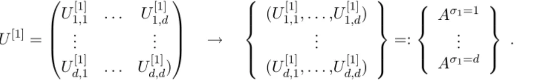
can also be interpreted as a set of d matrices of dimension 1 × d , cf. Fig. 2.2

U

=









U

. . . U

... ...

U

. . . U

)









→



 



 



(U

, . . . ,U

) ...

(U

, . . . ,U

)



 



 



=:



 

  A

...

A



 

 

. (2.30)

Next, the product S

V

is dened as a new d

× d

dimensional matrix Ψ

S

V

α1,(σ2,...,σL)

:= Ψ

1,σ2),(σ3,...,σL)

(2.31) that can again be decomposed by SVD. The index in square brackets marks both the step in the decomposition process and the lattice site that the leftover U

is associated with.

Carried out over all σ

this results in c

= Ψ

1),(σ2,...,σL)

= h

U

S

V

i

(σ1),(σ2,...,σL)

(2.32a)

=

d

X

α1=1

U

S

V

1,(σ2,...,σL)

(2.32b)

=: X

α1

A

1

Ψ

1,σ2),(σ3,...,σL)

(2.32c)

= X

α1

X

α2

A

1

U

1,σ2),α2

S

V

2,(σ3,...,σL)

(2.32d)

=: X

α1,α2

A

A

Ψ

2,σ3),(σ4,...,σL)

= · · · (2.32e)

= X

α1,α2,...,αL−1

A

A

· · · A

· · · A

A

(2.32f) Figure 2.1 shows how the big blob c

is decomposed into sets of local matrices A

that are associated with one lattice site each.

Figure 2.1: Left to right decomposition of the coecient vector c

into local sets of matrices A

. The colors indicate which matrices in Eq. (2.32) are associated with which lattice site.

The set of equalities (2.32) shows that every coecient c

for a given physical

conguration {σ

,σ

, . . . ,σ

} of the system can be obtained by choosing the right matrix

A

for every site and carrying out the matrix product. This leads to the

Denition: Matrix product state (MPS): Each state |ψi of a quantum mechani- cal system can be written as

|ψi = X

σ1,σ2,...,σL

A

· A

· · · A

|σ

,σ

, . . . ,σ

i (2.33) where A

is a set of local matrices with one element for each possible state of the quantum number σ

.

Note that no explicit knowledge about the basis |σ

,σ

, . . . ,σ

i is required other than ex- istence and ortho normality (which will be assumed as given).

By construction the dimension of the matrices A

is d

×d

, i.e. the maximum dimension in at i =

, growing exponentially with L . In some cases the Schmidt rank r

(number of non-zero singular values of Ψ

) can be smaller than the full dimension of S

, which leads to somewhat smaller matrix sizes.

The true potential of the MPS formalism is however, that by choosing a xed maximum matrix size of D , the number of parameters for a variational description can be reduced from O(d

) to O(LdD

) . This happens in a systematic fashion, because all the sites in the bulk of the chain are inuenced by this truncation in the same way.

An intuitive way of truncating the matrix size is to keep only the D largest singular values S

in each step. This is also optimal in a certain sense as will be shown in Sect. 2.2.5.

Obviously, the approximation is the better, the faster the decrease in the S

is. This approach is however inherently asymmetric as apparent from the construction method shown above. The truncation on bond (`) − (` + 1) inuences the sites to the right but not those to the left whose matrices have already been truncated.

2.2.2 Tensor network notation

As the formulation of the required matrix products in terms of sums over multiple indices, e.g. Eq. in (2.32), is rather cumbersome, a graphical, more intuitive representation is introduced.

The tensor network notation describes n -dimensional tensors as objects (e.g. circles, squares) with n legs sticking out, one for each free index.

An element of a local matrix A

`

is addressed by three indices σ

, α

and α

. This can also be understood as a tensor of rank 3 , giving rise to the pictogram for local matrices A

in Fig. 2.3.

In a tensor network solid lines connecting two objects represent indices that are contracted, i.e. summed over.

The example in Tab. 2.1 shows the computation of the trace Tr(AB) of a matrix product in tensor network notation where A and B are matrices of suiteable dimensions. The result is an object with zero free indices, i.e. a scalar.

In this notation, the expansion coeent in Eq. (2.33) looks like

c

= . (2.34)

Figure 2.2: Graphical representation of re-casting the left SVD factor U

into a set of d local matrices A

.

Figure 2.3: Tensor network representation of local matrices A

at the edges and in the bulk of the chain. The matrcies at the edges are simply vectors and therefore have only one matrix index α

and α

respectively. Complex conjugates that arise in the description of bra-vectors are depicted with a downward pointing physical index.

Table 2.1: Examples on tensor network notation

A, B 2 indices each

(AB)

= X

k

A

B

2 indices

Tr(AB) = X

j

(AB)

0 indices

2.2.3 General properties

The form of the MPS constructed in (2.32) is called left-canonical, as it is constructed

from left to right. By construction this form is also left-normalized, i.e. at each site i the

matrices A

satisfy

d

X

σi=1

A

A

= U

U

= 1 ∀ i , (2.35) but in general

X

σi

A

A

= U U

6= 1 . (2.36) Equation (2.35) implies that

hψ|ψi = 1 . (2.37)

While the left-canonical construction is intuitive, it is by no means the only possibility.

One can as well start the decomposition from right to left and in this case interpret the V

as a set of d local matrices B

c

= Ψ

1,...,σL−1),(σ_L)

(2.38a)

= X

αL−1

U

1,...,σL−1),αL

S

V

(2.38b)

= X

αL−1

Ψ

1,...,σL−2),(σL−1,αL−1)

B

= · · · (2.38c)

= X

α1,...,αL

B

1

B

· · · B

B

L,1

(2.38d)

= . (2.38e)

The representation obtained this way is then right-normalized:

d

X

σi=1

B

B

= V

V

= 1 ∀ i . (2.39) A third possibility is the mixed-canonical representation, where the decomposition is car- ried out form both the left and the right side. In this case, there is a leftover matrix S

containing the singular values on the bond between the left-canonical and the right- canonical parts.

c

= . (2.40)

To see how Eq. (2.35) and (2.39) imply normalization of the state consider the norm hψ|ψi

hψ|ψi = (2.41a)

= X

σ1,σ2,...,σL

c

c

= c

c

(2.41b)

= X

σ1,σ2,...,σL

(A

· · · A

)(A

· · · A

) (2.41c)

= X

σL

A

· · · X

σ1

A

A

!

| {z }

1

· · · A

= 1 (2.41d)

and for right-canonical MPS analogously. For mixed-canonical MPS the norm is hψ|ψi = Tr

"

X

σ1,σ2,...,σL

B

· · · B

S

A

· · · A

A

· · · A

S

B

· · · B

#

(2.42a)

= (2.42b)

= Tr(S

S

) . (2.42c)

From here on the local matrices will be labelled M

if the left- or right-canonical proper- ties are not used explicitly.

This shows, that the matrix product representation is not at all unique. And there are still many more gauge degrees of freedom which change the representation but not the state

|ψi . On each bond an invertible matrix X

can be introduced and the transformation M

→ M

X

, M

→ (X

)

M

(2.43) leaves the MPS invariant. Fixing all X

and the boundary conditions makes the state unique.

So far, only a chain with open boundary conditions (OBC) has been discussed. In this case, the matrices at the edges of the chain were simply vectors, thus making the complete product a scalar value c

. Since the matrices at each site i carry information about the interaction with all sites to the left (or to the right), in a chain with periodic boundary conditions (PBC) all matrices must have dimensions greater than 1 . For translationally invariant systems all matrices are of the same size. This will make the product itself a matrix instead of a scalar. The solution to obtain a scalar again is rather intuitive, looking at the tensor network

→ . (2.44)

The example on tensor networks in Tab. 2.1 shows that the long line coupling the end of the chain to its rst site corresponds to the trace operation. Thus for PBC, the coecients are

c

= X

σ1,σ2,...,σL

Tr(M

· · · M

) . (2.45) This form also holds for OBC, since the trace of a scalar is still the same scalar.

Thus for OBC the coecients are automatically scalars and PBC can be expressed by a trace operation which can be seen from the tensor network. There are however, other possible boundary conditions e.g. antiperiodic, xed or linear combinations of any of these.

Particularly for variational algorithms it is desireable to have the same xed matrix size

D on each lattice site independently of the boundary conditions. This leads to a more

general ansatz.

Denition: General ansatz for variational MPS: Each physical state |ψi of a one- dimensional system can be approximated variationally by

|ψ

i =

D

X

α,β=1

X

σ1,σ2,...,σ_L

a

M

· M

· · · M

b

|σ

,σ

, . . . ,σ

i (2.46) where the M

are D×D matrices and the a

and b

are D -dimensional column vectors.

The choice of the vectors a

and b

, which may depend on each other, provides the neces- sary degrees of freedom to implement various boundary conditions. For instance, the trace operation for PBC follows from a choice of, e.g., a

= e

and b

= δ

e

where the e

are Cartesian unit vectors. A concrete method to derive the a

and b

for particular boundary conditions will not be elaborated at this point, because it is not required for the presented method.

As an example let us consider the overlap hφ|ψi of two dierent states of the system, where the state |ψi is described by local matrices M

and |φi is described by M ˜

. Then

hφ|ψi = X

σ1,σ2,...,σL

c

c

(2.47a)

= X

σ1,σ2,...,σL

Tr( ˜ M

· · · M ˜

) Tr(M

· · · M

) , (2.47b) which is true for both OBC and PBC. In this form, there are d

products of 2L matrices each, so that the overall computational eort is O(Ld

) which is exponentially expensive.

However, most of the operations are unnecessary, because only two matrices change in each product. Therefore, a better way is to evaluate the expression as

hφ|ψi = (2.48a)

= X

σ1,σ2,...,σL

Tr( ˜ M

· · · M ˜

) Tr(M

· · · M

) (2.48b)

= X

σ1,σ2,...,σL

Tr h

( ˜ M

· · · M ˜

) ⊗ (M

· · · M

) i

(2.48c)

= Tr

"

X

σ1

M ˜

⊗ M

!

· · · X

σL

M ˜

⊗ M

!#

, (2.48d)

where ⊗ denotes the tensor product.

In this way, there is one product of L matrices of dimension D

× D

, which results in a total computational eort of O(dLD

) and the actual growth is only linear in the system size.

While the form in Eq. (2.48d) follows naturally from Tr(A)Tr(B) = Tr(A ⊗ B), this shows that the tensor product is the correct form of product to use when contractig over physical indices.

2.2.4 Matrix product operators (MPO)

Now that the matrix product form for quantum states has been dened, a compatible denition for operators is needed. States are dened by their expansion coecients

c

= hσ

,σ

, . . . ,σ

|ψi = M

· · · M

, (2.49)

where the M

are tensors of order 3. Correspondingly, operators are dened by their matrix elements which for a product of local operators are given by

hσ

, . . . ,σ

| O ˆ |σ

, . . . ,σ

i = W

· · · W

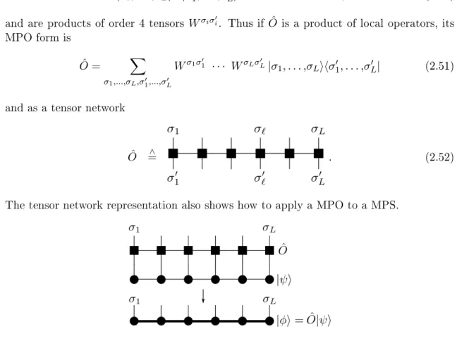
, (2.50) and are products of order 4 tensors W

. Thus if O ˆ is a product of local operators, its MPO form is

O ˆ = X

σ1,...,σL,σ⁰₁,...,σ⁰_L

W

· · · W

|σ

, . . . ,σ

ihσ

, . . . ,σ

| (2.51) and as a tensor network

O ˆ =

. (2.52)

The tensor network representation also shows how to apply a MPO to a MPS.

Figure 2.4: Application of a matrix product operator to a matrix product state As shown in Fig. 2.4, the network is contracted over the physical indices σ

, where the product form to be used is the direct matrix product

|φi = ˆ O |ψi = X

σ1,σ2,...,σL



 X

σ⁰₁

W

⊗ M



 · · ·



 X

σ_L⁰

W

⊗ M



 |σ

,σ

, . . . ,σ

i

= X

σ1,σ2,...,σL

N

· · · N

|σ

,σ

, . . . ,σ

i , (2.53) in analogy to the overlap in Eq. (2.48). This means that the dimension of the local ma- trices N

describing the new state |φi are of dimension D · D

× D · D

, where D

is the dimension of the operator matrices W

. This multiplication of matrix dimensions is denoted by the thicker lines in the diagram.

At this point one usually has to solve two issues: First, how to explicitly construct the matrices W

and sencond, how to reduce the matrix dimension of N

to D × D. There are systemic ways to do this. The construction and use of general MPOs is known as MPO formalism and the latter as MPS compression. Both are discussed in Ref. [26].

However, this general case is not really applicable for our method, as it deals with innte

systems. Also, as will be shown in detail in Chap. 3, it is not necessary.

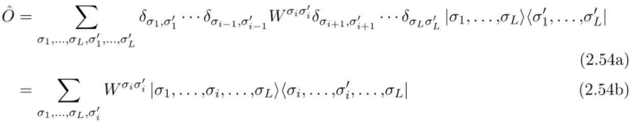
As a simple example, take the case of a matrix element hφ| O ˆ |ψi , where O ˆ is nontrivial only on a single lattice site i . In this case the MPO form is simple

O ˆ = X

σ1,...,σL,σ₁⁰,...,σ⁰_L

δ

1

· · · δ

i−1

W

δ

i+1

· · · δ

L

|σ

, . . . ,σ

ihσ

, . . . ,σ

| (2.54a)

= X

σ1,...,σL,σ_i⁰

W

|σ

, . . . ,σ

, . . . ,σ

ihσ

, . . . ,σ

, . . . ,σ

| (2.54b)

In the local Hilbert space of a single site the operator O ˆ and therefore W

is just a d × d matrix O . Thus

hφ| O ˆ

|ψi = (2.55a)

= Tr



 X

σ1

M ˜

⊗ M

!

· · ·



 X

σiσ⁰_i

O

0 i

i

M ˜

⊗ M



 · · · X

σL

M ˜

⊗ M

! 

 . (2.55b) Because the Hamiltonian (2.1) only consists of products of local operators, this is all that is required for our method at this point.

2.2.5 Connection to DMRG

For readers familiar with the DMRG method it is insctructive, to see how the two concepts connect. This section also shows, that DMRG's density matrix criterion is equivalent to truncating the singular values on each bond in a MPS construction and that this approach is optimal in a certain sense.

In his paper from 1992 [1], White started from two main ideas: First, in truncating the dimension of a Hilbert space, it is best not to keep the lowest energy states but the most probable ones. Secondly, an approximate state | ψi ˜ optimally represents the expectation values, i.e., the physics of the real state |ψi , if the deviation

S :=

|ψi − | ψi ˜

2

(2.56)

between them is minimal. Both lead to the same DMRG formalism that can be elegantly formulated using MPS.

We recall the way chain models are usually handled in numerical renormalization methods.

A given system of length ` is recursively expanded to size ` + 1 by adding a single lattice site as shown in Fig. 2.5.

Figure 2.5: Handling of chain models in numerical renormalization methods:

The system is built up by adding one site at a time.

Once the dimension of the Hilbert space reaches a certain limit, the basis of the newly formed block A

is truncated using a suiteable criterion. A major drawback in Wilson's NRG for chain models was the poor handling of the boundary conditions in the build up of such blocks. White solved this by means of his superblock ansatz.

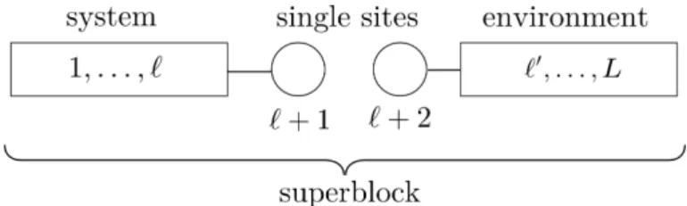
In addition to increasing the system size in each step, he added another block called environment. System and environment together form the superblock (see Fig. 2.6). Then, the Hamiltonian of this superblock is diagonalized and its states are projected onto the system block. This has the advantage that at the time site ` + 1 it is added to the system, is not a free end but a site in the bulk of a larger system.

Figure 2.6: Expansion scheme in standard DMRG: In each step one (or two) sites are added. System and environment are combined into the superblock.

Note that, as Fig. 2.6 shows, one can also add an additional site to the environment block at each step. A comment on terminology is in order at this point. In applications, the physical system of interest is the superblock (sometimes also called world). The splitting in system and environment is methodical, not physical.

The question is now how to project the superblock states onto the extended system block and how to truncate the system block basis to avoid exponential growth. Both questions lead to the use of the density matrix, more precisely to the reduced density matrix of the system block (of length ` + 1 ).

For simplicity the superblock will be assumed to be in a pure state |ψi , but the argument also holds for mixed states [34]. Let { |ii} with i = 1, . . . ,d

be a complete orthonormal basis of the system's Hilbert space and { |ji} with 1, . . . ,d

one of the environment's Hilbert space. Then the superblock state is given by the product state

|ψi =

d_S

X

i d_E

X

j

ψ

|ii ⊗ |ji = X

ij

ψ

|ii |ji with ψ

= hj|hi|ψi . (2.57)

Consider an observable operator that acts only on the system block and is the identity on the environment. Its spectral representation is

A

= A

⊗ 1

= X

ii⁰j

A

|ii |jihj|hi

| . (2.58)

Its expectation value with respect to |ψi is

hAi = hψ|A

⊗ 1

|ψi = hψ|



 X

ii⁰j

A

|ii |jihj|hi

|



 |ψi (2.59)

= X

i⁰⁰j⁰⁰

X

i⁰⁰⁰j⁰⁰⁰

X

ii⁰j

ψ

ψ

A

hj

|hi

|ii |jihj|hi

|i

i |j

i (2.60)

= X

ii⁰j

A

ψ

ψ

= X

ii⁰

A

X

j

ψ

ψ

(2.61)

= Tr(ρA) . (2.62)

The last equality denes the object

ρ

= X

j

ψ

ψ

(2.63)

as the reduced density matrix of the system block. This matrix holds all information of the superblock state |ψi needed to compute the expectation value of any A that acts only on the system.

Let the eigenvalues of ρ be w

and the corresponding eigenvectors |u

i . The |u

i form a valid basis of the system block Hilbert space because as a density matrix ρ is hermitian and positife-semindenite. The w

are assumed to be ordered w

≥ · · · ≥ w

. By denition of the density matrix, the eigenstates with the largest w

are the most probable states. If, in accordance with the initial idea, the D most probable states

of the system block are kept, the approximate superblock state can be rewritten as

| ψi ˜ =

d_E

X

j D<d_S

X

α

a

|u

i |ji = X

α

|u

i X

j

a

|ji = X

α

a

|u

i |v

i . (2.64) Thus, the expansion coecient ψ ˜

with respect to the complete basis |ii |ji is given by

ψ ˜

:= hj|hi| ψi ˜ = X

α

a

hi|u

ihj|v

i = X

α

a

u

v

. (2.65) Note that this has the form of an element in a product of three matrices (U AV

)

, where A is a diagonal matrix with A

= a

. In terms of the expansion coecients the deviation S becomes

S = X

ij

ψ

− ψ ˜

2

= X

ij

ψ

− X

α

u

a

v

2

(2.66) or on a matrix level

S =

Ψ − U ˜ A ˜ V ˜

2

F

(2.67)

where the F denotes the Frobenius norm. This form of Ψ ˜ looks very much like the SVD from theorem 2.1. Indeed, linear algebra proves S to be minimal if U ˜ A ˜ V ˜

is chosen as the SVD of ψ ˜

interpreted as d

× d

matrix. Details can, e.g., be found in Ref. [35].

By construction, V ˜

describes the environment block and U ˜ the system block. The a

are the singular values on the bond connecting the two parts. Also, by the properties of the SVD U U

= 1 and V

V = 1. This is exactly the form of a mixed canonical MPS as seen

2In DMRG literatureD is referred to asmmost times.