When does a disaster become a systemic event? Estimating indirect economic losses from natural disasters

Estimating indirect economic losses from natural disasters

Sebastian Poledna

, Stefan Hochrainer-Stigler

, Michael Gregor Miess

, Peter Klimek

, Stefan Schmelzer

, Johannes Sorger

, Elena Shchekinova

, Elena Rovenskaya

, Joanne Linnerooth-Bayer

, Ulf Dieckmann

, and Stefan Thurner

1

International Institute for Applied Systems Analysis, Schlossplatz 1, 2361 Laxenburg, Austria

2

Complexity Science Hub Vienna, Josefst¨ adter Straße 39, 1080 Vienna, Austria

3

Section for Science of Complex Systems, Medical University of Vienna, Spitalgasse 23, 1090 Vienna, Austria

4

Santa Fe Institute, 1399 Hyde Park Road, Santa Fe, NM 87501, USA

5

Institute for Advanced Studies, Josefst¨ adter Straße 39, 1080 Vienna, Austria

6

Faculty of Computational Mathematics and Cybernetics, Lomonosov Moscow State University (MSU), Moscow, Russia and

7

Vienna University of Economics and Business, Welthandelsplatz 1, 1020 Vienna, Austria

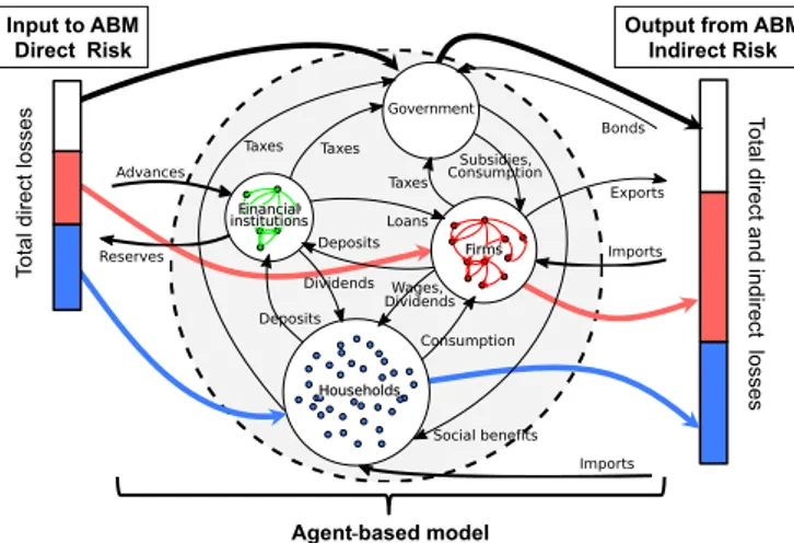
Reliable estimates of indirect economic losses arising from natural disasters are currently out of scientific reach. To address this problem, we propose a novel approach that combines a probabilistic physical damage catastrophe model with a new generation of macroeconomic agent-based models (ABMs). The ABM moves beyond the state of the art by exploiting large data sets from detailed national accounts, census data, and business information, etc., to simulate interactions of millions of agents representing each natural person or legal entity in a national economy. The catastrophe model introduces a copula approach to assess flood losses, considering spatial dependencies of the flood hazard. These loss estimates are used in a damage scenario generator that provides input for the ABM, which then estimates indirect economic losses due to the event. For the first time, we are able to link environmental and economic processes in a computer simulation at this level of detail.

We show that moderate disasters induce comparably small but positive short- to medium-term, and negative long-term economic impacts. Large-scale events, however, trigger a pronounced negative economic response immediately after the event and in the long term, while exhibiting a temporary short- to medium-term economic boost. We identify winners and losers in different economic sectors, including the fiscal consequences for the government. We quantify the critical disaster size beyond which the resilience of an economy to rebuild reaches its limits. Our results might be relevant for the management of the consequences of systemic events due to climate change and other disasters.

Keywords: resilience

large-scale data-driven modeling

economic simulator

natural hazard modeling

environmental-economic coupling

I. INTRODUCTION

Total economic losses from natural and man-made dis- asters in 2017 are estimated to be USD 306 billion.

With hurricanes Harvey, Irma and Maria, which have made 2017 the second costliest hurricane season on record, the US was hit particularly hard. Due to climate change, economic losses from extreme events – such as floods, droughts, and other climatic disasters – will further in- crease, and events that have been considered rare until now will become more common in the future [1]. How- ever, the resulting economic losses to a national econ- omy are difficult to quantify. While direct losses due to the immediate destruction of homes, firms, infrastruc- tures and lives can be reliably estimated with existing data, estimates of indirect losses – which arise as eco- nomic consequences of physical destruction – are much harder to obtain, and no consensus on their validity exists [2]. The primary reason for this is that natural disasters affect the economy in multiple ways and along several

1 http://www.swissre.com/media/news_releases/nr20171220_

sigma_estimates.html

dimensions [3, 4]. For example, a flood event might de- stroy or damage the physical capital of a firm, causing output losses and worker layoffs. This, in turn, can trig- ger further output losses to suppliers and customers of that firm, potentially leading to more layoffs. The asso- ciated reduction in household income additionally lowers consumption, potentially further enhancing output losses and increasing layoffs. Subsequently, however, the recon- struction of damaged or destroyed capital can have the opposite effect: companies involved in reconstruction ac- tivities experience growth and expand their workforce, which results in higher income that ripples through the economy and leads to economic growth via Keynesian multiplier effects. Hence, natural disasters simultane- ously cause both indirect losses and indirect gains. We refer to these losses and gains as indirect economic ef- fects.

2

To avoid double counting, we measure losses or gains as the change in gross domestic product (GDP) relative to a baseline scenario. This definition differs from [5], who additionally at- tributes employment losses (e.g. due to the closure of damaged facilities) to direct losses, and defines indirect losses as all eco- nomic consequences except for damages (direct losses) and em- ployment losses caused by the disaster.

arXiv:1801.09740v1 [q-fin.EC] 29 Jan 2018

Indirect economic effects of average natural disasters, as measured by changes in GDP, are typically small. Net effects may even be close to zero in the short term, where losses and gains of natural disasters can cancel each other out [6]. Still, there are winners and losers, since effects may differ substantially across industries and economic sectors, and almost never cancel for companies and indi- viduals [7]. Several empirical studies even find small but positive short- to medium-term overall effects for moder- ate natural disasters of certain types, especially for mod- erate floods [7–14]. However, the evidence on the sign and magnitude of indirect economic effects of natural disasters in general remains mixed and conflicting, see [11–13] for recent surveys. This situation is echoed in meta-analyses such as [15], which reports that disasters on average have an insignificant impact in terms of in- direct costs, and [16], which finds some evidence that a part of the negative impact of natural disasters reported in studies is caused by a publication bias. Moreover, [17] shows that the impacts of natural disasters on differ- ent components of GDP (such as investment, government and private consumption, exports, imports) differ widely in timing, direction and extent. More aggregate analy- ses might mask these differences, and it may be difficult to find clear and large net aggregate impacts on GDP.

Severe natural disasters (systemic events), on the other hand, are not believed to have neutral or positive eco- nomic effects on an aggregate level [7–9, 12, 18, 19]. In- direct economic losses from these systemic events may be amplified by several mechanisms such as post-disaster in- flation, network effects like supply chains affecting firms that were not initially impacted by the event, as well as physical and financial resource constraints regarding the productive capacity of the economy [3]. Despite these general arguments, empirical evidence on indirect economic effects of systemic events, particularly regard- ing severe floods in developed economies, is scarce and largely inconclusive [7–10, 20, 21].

Indirect economic effects from natural disasters are dif- ficult to model with traditional approaches such as input- output (IO) models [22–28], computable general equilib- rium (CGE) models [29–34], and econometric analyses [7–19, 35] because of the over-simplifying nature of these approaches [36]. IO models have a tendency to overes- timate indirect economic losses and gains [2]. This was demonstrated, for example, for the case of job gains from reconstruction following the Northridge earthquake in California in 1994: [37] showed that the IO estimates by [38] significantly exceeded actual data for the Los Angeles area following the earthquake [2]. Furthermore, IO mod- els cannot incorporate the reactions of economic agents to a disaster. By design, CGE models are overly optimistic regarding the flexibility of an economy to react to natural disasters [3]. This is due to the underlying assumption that price clearing mechanisms bring the economy back to a general equilibrium after a certain time and are sub- ject only to modest constraints such as adjustment costs in the investment function. However, real-world price

formation is sticky and imperfect. Production functions typically assumed in CGE models

often overstate the flexibility of substitution between factors of production (labor, capital, material input). Econometric analysis of indirect economic effects faces the problem that statis- tical, historical relationships used to derive model pa- rameters are likely to be disrupted by the disaster [2].

The latter study points out an array of factors that may challenge the implicit socio-economic assumptions of the approach, including: the temporary nature of measures taken directly after the disaster event, permanent eco- nomic changes (e.g. in the production function), pur- chase and sale patterns, as well as labor force migration or overtime hours in the reconstruction phase. Indicative of this, [6] demonstrates that the regional econometric model results in [39] over-estimated the economic impact of Hurricane Andrew, which hit the US in 1992, by 70-85

% [2].

In summary, traditional approaches so far have failed to provide unambiguous conclusions about the indirect economic effects of natural disasters, in particular re- garding systemic events. This means that, given the characteristics of these traditional approaches, today it is still largely impossible to relate the size of initial dam- ages of natural disasters to the expected subsequent indi- rect economic effects, or to clearly disentangle expected losses and growth effects on a sectoral level. To address this problem, we propose a novel approach that combines a probabilistic physical damage catastrophe model with a new generation of macroeconomic agent-based models (ABMs). The ABM we adopt moves beyond the state of the art by exploiting large data sets from detailed na- tional accounts, census data, and business information, etc., to simulate the interactions of millions of agents rep- resenting each natural person or legal entity, such as cor- porations, government entities and institutions in a na- tional economy. It has been shown that this model is able to forecast numerous macroeconomic variables including major variables such as GDP, inflation, consumption and investment better than standard forecasting approaches [40].

We apply our method to estimate indirect economic losses from flood events in Austria, for which the men- tioned data is available in highly detailed, complete and consistent form (see SI

). The ABM is geolocalized in the sense that the location of capital stock, e.g. firms and infrastructure, is known. The geospatial distribution of capital across Austria is shown in Fig. 1. The physi- cal damage catastrophe model (damage scenario genera- tor) allows us to generate realistic virtual natural disaster events (floods) of controlled size. It is based on a copula approach that assesses realistic hazard frequency and in- tensity, and takes into account spatial dependencies and

3

Constant elasticity of substitution (CES) functions.

4http://www.complex-systems.meduniwien.ac.at/people/

spoledna/supporting_information_poledna_et_al_2018.pdf

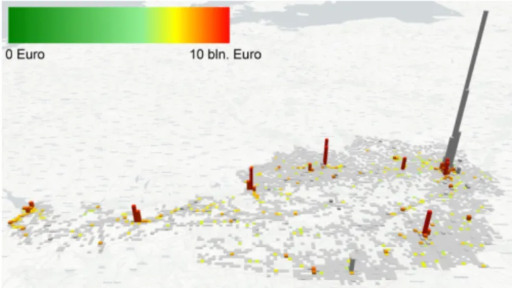
FIG. 1. Geospatial distribution of capital across Austria. Af- fected capital in flooding zones of a 250-year event is shown in a color scale from green to red, where green indicates small damages and red large damages up to 10 bln. Euro. Gray indicates capital stock not affected by the flood. For exam- ple, capital stock in Vienna (the large bar in the northeast) is not affected due to extensive flood protection measures, and is therefore shown as grayed out.

the dependency on the severity of the events (see SI). Af- ter generating a geolocalized flood event of a given size at the beginning of year 2014,

the affected dwellings, firms and infrastructure are destroyed (the affected cap- ital in flooding zones of a 250-year event is depicted in Fig. 1). On this basis, the detailed indirect economic effects across economic sectors and industries are studied in the ABM over several consecutive years.

RESULTS

Moderate disasters do not always have a negative impact on economic growth

Fig. 2 shows the indirect economic effects resulting from a 100-year (blue line) and a 250-year (red line) flood event that destroys dwellings and productive capital.

The total direct losses (damages) amount to about 0.6

% (100-year event) and 1.2 % (250-year event) of Aus- trian capital stock, respectively. Fig. 2(a) shows the cu- mulative change in the GDP growth rate relative to the baseline scenario

in percentage points (pp).

The qual-

5

This year is chosen to simulate the flooding event since 2013 it is the last year for which the main data source – the symmetric IO tables for the Austrian economy – is available to calibrate the model.

6

The event occurs at the beginning of the year 2014.

7

The baseline scenario describes a continuation of current trends for the Austrian economy. The baseline scenario serves as the benchmark against which we evaluate the indirect economic ef- fects of the different flooding scenarios.

8

A percentage point (pp) is the unit for the arithmetic difference of two percentages. For example, moving up from 10% to 12% is

2013 2014 2015 2016 2017 2018 2019 2020 2021 2022 2023 Year

-6 -5 -4 -3 -2 -1 0 1 2 3 4

Cumulative change in GDP-growth rate [pp]

(a) Baseline

100-year event 250-year event 1500-year event

2013 2014 2015 2016 2017 2018 2019 2020 2021 2022 2023 Year

-3 -2.5 -2 -1.5 -1 -0.5 0 0.5 1 1.5 2

Cumulative change in unemployment rate [pp]

(b)

2013 2014 2015 2016 2017 2018 2019 2020 2021 2022 2023 Year

-4 -2 0 2 4 6 8 10 12 14

Change in government debt-to-GDP ratio [pp]

(c)

FIG. 2. Indirect economic gains and losses of a 100- (blue),

250- (red) and 1,500- (black) year flood event. Time labels on

the x-axis indicate the end of each year, and the gray verti-

cal bar marks the first year after the flood. The panels show

the effects as percentage point changes relative to the base-

line scenario, in which no disaster happens. (a) Cumulative

changes in GDP-growth rates. (b) Cumulative changes in the

unemployment rate. (c) Changes in the government debt-to-

GDP ratio. Shaded areas cover one standard deviation above

and below the mean values, as obtained from 50 independent

Monte-Carlo simulations.

itative behavior of the two scenarios is similar: starting from small negative effects immediately after the disaster, cumulative effects on economic growth then become pos- itive in the short to medium term (2014-2018), and turn negative in the long term. These effects are most pro- nounced with an about 0.5 pp cumulative GDP growth rate increase (250-year event) relative to the baseline sce- nario in the second year after the flood (2015). In the long term, primarily due to a multiplier-accelerator mecha- nism [41] (see below), the effects decline to an almost neutral impact (100-year event), and to a reduction of GDP growth of approx. 0.8 pp (250-year event), respec- tively. This behavior, i.e. positive short- to medium-term and negative long-term effects of moderate size, is in line with the literature [7, 8, 10, 14, 35]. Fig. 2(b) demon- strates that – as to be expected according to Okun’s law – the change in the unemployment rate is inversely cor- related to economic growth, but at a slightly lower am- plitude: for the 250-year event, a cumulative decline of almost 0.5 pp two years after the flood (2015) is followed by a cumulative growth in the unemployment rate up to a maximum of about 0.5 pp in the long term. Fig. 2(c) de- picts the government debt-to-GDP ratio and shows that the dynamics of the growth and unemployment rates, as well as the transfer we assume to be provided by the gov- ernment to fully compensate households for their losses of dwellings as catastrophe relief, all lead to an initial rise in this ratio of about 2 pp. For three years after the flood (2015-2018), the government debt-to-GDP ra- tio temporarily falls slightly below its initial level, but in the long run stabilizes at an increase by more than 2 pp relative to the baseline scenario (250-year event).

Severe disasters have pronouncedly negative economic effects immediately after the event and in

the long term

A severe-disaster scenario that simulates a 1500-year flood event is shown in Fig. 2 (black lines). The to- tal direct losses correspond to approximately 10 % of the capital stock in Austria. The indirect economic ef- fects after this shock are qualitatively different from the moderate-disaster scenarios. The initial overall effect on GDP growth is pronouncedly negative, with a cumula- tive reduction of GDP growth by about 5 pp, see Fig.

2(a). Due to reconstruction, growth picks up fast in the year after the disaster, and surpasses cumulative GDP growth of the baseline scenario by the second year after the flood (2015), culminating in a temporary economic boost of about 2 pp of additional cumulative GDP growth in 2016. The multiplier-accelerator mechanism [41], as well as production, capacity and credit constraints (see SI) drag growth downwards after this point, leading to

a 2 pp increase, but it is a 20 percent increase in what is being measured.

2013 2014 2015 2016 2017 2018 2019 2020 2021 2022 2023 Year

-5 -4 -3 -2 -1 0 1 2 3 4 5 6 7 8

Cumulative change in GDP-growth rate by sector [pp]

Real estate Construction Manufacturing

FIG. 3. Cumulative growth effects on sectoral GDP after a 250-year flood event for selected economic sectors in per- centage points (pp) relative to the baseline scenario. Shaded areas cover one standard deviation above and below the mean values. Sectors shown: construction sector (black), manufac- turing sector (red) and real estate sector (blue). The gray vertical bar indicates the year of the flood.

negative long-term cumulative growth effects of approx.

1.7 pp. The unemployment rate reacts strongly to the se- vere disaster, with a cumulative initial increase of more than 1.5 pp, and is followed by a reduction up to al- most 2 pp in 2015 during the reconstruction phase, see Fig. 2(b). After this pronounced disruption of the labor market, the unemployment rate rises again by a cumula- tive change of approx. 0.5 pp (2020) due to the cyclical dynamics, and stabilizes at a level close to the baseline scenario in the long term. Immediately after the disas- ter, a large initial government transfer to households to compensate for their losses of housing stock,

as well as substantial decreases in government revenues and GDP, lead to a 10 pp rise of the government debt-to-GDP ra- tio, see Fig. 2(c). Even though this ratio shortly returns to its initial level due to the positive economic effects of reconstruction, the downturn because of over-production three years after the flood event implies a subsequent rise in this ratio by almost 10 pp, leaving government finances substantially deteriorated in the long term.

9

We assume – in line with past experiences of political processes

regarding catastrophe relief by the Austrian government – this

transfer to be limited to about a third of the total losses in

dwelling stock.

Effects differ substantially across industries and economic sectors

While moderate flood events can have positive aggre- gate effects in the medium term, impacts are expected to differ significantly across economic sectors. Fig. 3 confirms this conjecture. It shows the effects for the most severely impacted sectors as a result of the 250-year event. The real estate sector (blue line) suffers substan- tially from the destruction of residential capital stock:

sectoral output is reduced by more than 4 pp. Despite reconstruction works improving the initial situation, the cumulative growth change in this sector remains nega- tive, with a cumulative loss in growth of about 2 pp in the long run. The construction sector (black line) imme- diately profits from the reconstruction of dwellings and productive capital with a sectoral GDP growth of almost 6 pp in the first year after the flood (2014). After the fast ramp-up of reconstruction during the first years af- ter the flood, peaking in an about 6.5 pp increase in the second year after the flood (2015), this effect gradually wears off in the following years, turns slightly negative by year seven after the flood (2020) and remains rather sta- ble at this level thereafter. The restoration of productive capital takes more time. The largest cumulative increase for the manufacturing industry (red line) of about 1 pp is reached in year two after the flood (2015), since this sector supplies a major part of the material input for the re-installment of losses in productive capital. Follow- ing the general downturn due to over-production and the thereby induced economic cycle, we see that cumulative GDP growth of this sector in the long term (2019-2023) is lower by almost 1 pp than in the baseline scenario. The effects on all sectors can be found in Table S7 in the SI.

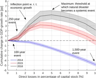
Loss of resilience – when disasters become systemic events

Fig. 4 shows the cumulative changes in GDP growth (relative to the baseline scenario) as a function of the sizes of direct damages of the event for different times after the disaster: one year (2014), two years (2015), and three years (2016) after the flood event. As can be ex- pected, the larger the direct damage, the larger the de- cline of GDP growth immediately after the flooding dis- aster (2014) is. In the second year after the flood event (2015), the effects of increased economic activity induce positive overall GDP growth. Within this second year, a large part of the initial damage can already by com- pensated, i.e. cumulative growth effects in the second year are slightly positive, but remain below 1 % for dis- asters smaller than a 250-year event. For larger events, the economy shows a remarkable growth that is induced by reconstruction after the disaster, which clearly out- weighs the direct losses. This growth is limited by dif- ferent constraining factors (see SI) and starts to decline with respect to the direct losses inflicted by the disas-

0 1 2 3 4 5 6 7 8 9 10

Direct losses in percentage of capital stock [%]

-6 -5 -4 -3 -2 -1 0 1 2 3 4 5 6 7 8

Cumulative change in GDP-growth rate [pp]

2014 2015 2016

Inflection point w. r. t.

economic growth

250-year event

100-year event

1,500-year event Maximum: threshold at which natural disaster becomes a systemic event

FIG. 4. Cumulative changes in GDP growth relative to the baseline scenario as a function of the direct damage as a per- centage of GDP. Results are shown for three different years after the disaster: 2014, 2015 and 2016. Shaded areas cover one standard deviation above and below the mean values.

Immediately after the event (2014), all disaster sizes are asso- ciated with negative growth relative to the baseline scenario.

In contrast, for the years 2015 and 2016 there exist inflection points and maxima for GDP growth, indicating the existence of direct damage sizes that, respectively, are “optimal” in terms of economic growth and determine a threshold where natural disasters become systemic events.

ter: the inflection point of the curve occurs at about a 2.4 % loss of capital stock. The cumulative changes in GDP growth in this year show a maximum in the re- gion where the initial damage causes about 3-4 % direct losses in the capital stock. At this maximum, the growth effects lose momentum and indirect losses start to dom- inate beyond the maximum. The situation is similar for two years after the event (black line): while the posi- tion of the inflection point remains at about 2.4 %, the growth stimulus is somewhat more pronounced, and the maximum is located at approximately 5 % direct losses.

At this point economic growth is severely restrained, the ability for resilience is lost, and the natural disaster be- comes a systemic event.

DISCUSSION

We present a novel approach for estimating the indirect

economic losses caused by natural disasters by combining

a probabilistic physical damage catastrophe model with

a macroeconomic ABM. The method has been applied

to flood scenarios in Austria. The ABM is calibrated

to the Austrian economy (households, non-financial and

financial firms and a government sector) at a scale of

1:1, i.e. every economic agent in Austria (about 10 mil-

lion) is represented in the model. The ABM incorpo- rates an input-output model with 64 industries, where all goods and services are produced endogenously, and depicts the relevant constraints regarding productive ca- pacities and financing conditions at the level of individual agents. This allows us to estimate the indirect economic effects of natural disasters that are caused by the un- folding sequence of economic events following the initial destruction of productive capital and dwellings. In par- ticular, the model shows the indirect economic effects of simulated disaster shocks of controlled size on the Aus- trian economy in terms of cumulative GDP growth and other major macroeconomic variables

The model produces realistic results in a number of aspects. Specifically, results correspond well with recent empirical findings of studies including sectoral detail and different types of disasters such as [7, 8, 10, 14, 18, 35].

We find that moderate losses due to 100- and 250-year flood events have small but positive short- to medium- term impacts, while they lead to negative long-term ef- fects of similar magnitude. These results correspond par- ticularly well with [10], which shows that floods of mod- erate magnitude in developed economies, while resulting in positive short- to medium-term effects, have slightly negative cumulative effects in the long run. Short- to medium-term results are further supported by a firm- level empirical study on flooding disasters in Europe [14], which finds higher average firm asset and employment growth for regions affected by flooding disasters. Com- parable impacts are also obtained by [7, 8], which report aggregate short- to medium-term positive growth effects of floods, and by [18], which shows that natural disas- ters have positive short-term growth effects in developed economies. Negative long-term effects for climatic disas- ters are also reported in [35].

Our study is the first to estimate the indirect economic impacts of severe floods in a developed economy on an empirical basis, at the same time taking account of com- plex economic interactions and dynamics with our mod- eling approach. Simulations of severe disasters, such as a 1,500-year flood event in Austria, induce a pronouncedly more negative long-term economic impact on the Aus- trian economy. These results, in line with a theoreti- cal analysis conducted by [42], demonstrate that nega- tive indirect effects from severe disasters are primarily due to constraints on the productive capacity of the ex- isting capital stock, credit provision and government fi- nances, which impede immediate reconstruction and thus impose a ceiling on positive growth effects. Empirical findings regarding severe floods are largely inconclusive:

[7–10, 20, 21] all report no, insignificant or (once con- trolled for) vanishing effects for systemic floods in par- ticular. Especially regarding the most detailed study on flooding disasters [10], a lack of data on severe floods in developed countries seemed not to have permitted the obtaining of results for this country group.

A unique feature of this analysis is that disaster im- pacts are disaggregated across 64 industry sectors and si-

multaneously tracked over time, demonstrating how pos- itive aggregate economic consequences may result in win- ners and losers subject to particular dynamics. The sec- toral decomposition of results reveals that, while some sectors providing the means for the reconstruction of cap- ital stock might profit (predominantly the construction sector, to a lesser extent the manufacturing sector), oth- ers that are particularly hit by the disaster suffer from large losses that take several years to be compensated (especially the real estate sector). We compute the dis- tribution of losses and their dynamics over time across sectors at a higher level of detail than previous stud- ies. Models featuring endogenous dynamics such as CGE models, even though they depict up to 35 industry sectors as in [30], typically are comparative static CGE models

[30–32], while fully dynamic CGE models usually depict only one output good as in [29]. Furthermore, they often are confined to regions smaller than a national economy [31, 32]. Sectoral empirical studies such as [7, 8, 10] – be- sides being limited methodologically as set forth above – typically divide the economy into two to three aggregate sectors (agriculture, industry and/or service sector). IO models applied to comparable contexts, such as [23], usu- ally exploit the full range of national IO tables (mostly around 60-70 industries), but lack the endogenous non- linear dynamics present in the ABM.

We show that disasters trigger cyclical economic re- sponses that follow a classic multiplier-accelerator mech- anism as described in [43]. The cycle is caused by an over- shooting of investment during the reconstruction phase leading to an economic boom, which is followed by a downturn due to a lack of demand once the restora- tion of capital stock has been completed. As reported in [7, 8, 10], indirect economic effects immediately af- ter the event are predominantly negative due to initial losses of capital stock, income, as well as demand and supply of goods. The positive economic stimulus due to reconstruction occurs with a delay of at least a quar- ter, because some time is necessary to compensate for lost capital stock and income. This impulse in turn trig- gers an economic cycle. In the long term, the conse- quences of this cycle tend to outweigh the positive eco- nomic impact induced by reconstruction activities. Such a cyclical mechanism – which is different from Schum- peter’s creative-destruction or productivity effect, which has been the focus of several studies

– has received little

10

I.e. they compare an initial equilibrium state before the disaster and another equilibrium state after the disaster without consid- eration of the dynamics between these two economic equilibria.

11

We do not consider this productivity effect in the present study,

since its empirical relevance is unclear and subject to extensive

debate in the literature, where different empirical studies present

mixed evidence on growth effects and associated increases in cap-

ital productivity after a natural disaster. For further discussion

on the productivity effect see [3], for empirical studies presenting

positive growth effects attributed to the productivity effect see

[44] and [45], whose findings are contradicted by several other

empirical studies, see [19, 20, 35, 46, 47].

Bonds

Social benefits Advances

Reserves

Taxes Taxes

Loans Deposits

Deposits Taxes

Imports Imports Exports

Consumption Dividends Wages,

Dividends Subsidies, Consumption

-

FIG. 5. Schematic overview of the ABM structure showing the institutional sectors (households, non-financial and finan- cial firms and a general government), and their interactions.

The stacked bars show an example of the distributions of di- rect (left) and indirect (right) total losses to the government (white), firms (red), and households (blue).

attention in the literature up to now, with the exception of a theoretical analysis in [48].

This study is the first to combine a probabilistic phys- ical damage catastrophe model with a macroeconomic ABM to quantitatively relate disaster sizes with the indi- rect economic impacts. We find a non-trivial behavior of the cumulative GDP growth effects as a function of the direct damage size. We determine a threshold beyond which the full productive capacity of an economy has been exploited to restore destroyed capital stock. At this point, which is at around 5 % of destroyed capital stock, resilience is lost, and economic growth is dominated by direct losses. Previous studies such as [42] have hith- erto investigated this matter on a theoretical and more aggregate basis only.

We believe that in times of increased frequency and severity of potential climate-change-related natural disas- ters, it is expedient to anticipate their short- to long-term economic implications, direct as well as indirect ones. In particular, it is important to identify potential economic losers of these events, so as to optimally prepare for a fair and efficient post-crisis management.

MATERIALS AND METHODS Agent based model of a small economy We employ an ABM – developed in [40] and [49] – which depicts the economy of a small nation at a 1:1 scale (about 10 million agents) (see SI for a model de- scription). The model is based on detailed data sources from national accounts, input-output tables, government statistics, census data and business surveys, and is able

to closely approximate time series of major macroeco- nomic variables (GDP, inflation, household consumption, investment). The basic structure of the model is depicted in Fig. 5. The model is calibrated to the economy of Austria in the year 2013, for which the required data is available (see SI). Large economies are still out of scope for such simulations within reasonable computing time.

Simulations were carried out on the supercomputer of the Vienna Scientific Cluster.

Flood risk estimation and damage scenario generator We estimate the disaster risk distributions for flood losses in Austria using a copula approach, and build a damage-scenario generator based on spatially explicit data to simulate losses to individual households, non- financial and financial firms and government entities across the 64 economic sectors represented in the ABM.

The damage-scenario generator simulates a shock to indi- vidual agents in the ABM, which subsequently alter their behavior and create higher-order indirect effects over a given time period (see SI).

ACKNOWLEDGMENTS

We acknowledge support from the EC H2020 project SmartResilience under grant agreement No 700621.

Computations were performed in part on the Vienna Sci- entific Cluster. We would like to thank Prof. Georg Pflug as well as Dr. Anna Timonina-Farkas for helpful com- ments in designing the modeling approach and providing useful inputs.

REFERENCES

[1] J. M. Melillo, T. Richmond, and G. Yohe, Third National Climate Assessment (2014).

[2] National Research Council, The impacts of natural dis- asters: A framework for loss estimation (National Academies Press, 1999).

[3] S. Hallegatte and V. Przyluski, The economics of natural disasters: concepts and methods, Tech. Rep. 5507 (The World Bank Policy Research Working Paper, 2010).

[4] I. Linkov, T. Bridges, F. Creutzig, J. Decker, C. Fox- Lent, W. Kr¨ oger, J. H. Lambert, A. Levermann, B. Mon- treuil, J. Nathwani, et al., Nature Climate Change 4, 407 (2014).

[5] H. C. Cochrane, in Modeling Spatial and Economic Im- pacts of Disasters (Springer, 2004) pp. 37–52.

[6] C. T. West, in Proceedings of Analyzing Economic Im- pacts and Recovery from Urban Earthquakes: Issues for Policy Makers, Conference presented by Earthquake Engineering Research Institute and Federal Emergency Management Agency, Pasadena, California (1996).

[7] N. V. Loayza, E. Olaberria, J. Rigolini, and L. Christi-

aensen, World Development 40, 1317 (2012).

[8] T. Fomby, Y. Ikeda, and N. V. Loayza, Journal of Ap- plied Econometrics 28, 412 (2013).

[9] E. Cavallo, S. Galiani, I. Noy, and J. Pantano, Review of Economics and Statistics 95(5), 1549 (2013).

[10] J. Cunado and S. Ferreira, Land economics 90, 149 (2014).

[11] E. Cavallo, I. Noy, et al., International Review of Envi- ronmental and Resource Economics 5, 63 (2011).

[12] C. Kousky, Energy Economics 46, 576 (2014).

[13] N. Shabnam, International Journal of Disaster Risk Sci- ence 5, 157 (2014).

[14] A. M. Leiter, H. Oberhofer, and P. A. Raschky, Envi- ronmental and Resource Economics 43, 333 (2009).

[15] S. Lazzaroni and P. A. van Bergeijk, Ecological Eco- nomics 107, 333 (2014).

[16] J. Klomp and K. Valckx, Global Environmental Change 26, 183 (2014).

[17] P. S. Mohan, B. Ouattara, and E. Strobl, Ecological Economics 146, 1 (2018).

[18] I. Noy, Journal of Development economics 88, 221 (2009).

[19] S. Hochrainer, World Bank Policy Research Working Pa- per 4968 (2009).

[20] I. Noy and A. Nualsri, University of Harvard Working Paper 07-28 (2007).

[21] C. R. Jaramillo, Documentos CEDE Universidad de Los Andes (2009).

[22] Y. Okuyama and J. R. Santos, Economic Systems Re- search 26, 1 (2014).

[23] S. Hallegatte, Risk analysis 28, 779 (2008).

[24] Y. Okuyama, Economic Systems Research 19, 115 (2007).

[25] A. Rose and J. Benavides, Advances in social science analysis of earthquakes, Buffalo, NY: National Center for Earthquake Engineering Research (1997).

[26] R. V. Whitman, T. Anagnos, C. A. Kircher, H. J. Lago- rio, R. S. Lawson, and P. Schneider, Earthquake Spectra 13, 643 (1997).

[27] R. Boisvert, Indirect economic consequences of a catas- trophic earthquake , 207 (1992).

[28] H. Cochrane, Menlo Park, CA: Risk Management Solu- tions (1997).

[29] H. Strulik, T. Trimborn, et al., Natural disasters and macroeconomic performance, Tech. Rep. (Vienna Uni- versity of Technology, Institute for Mathematical Meth- ods in Economics, Research Group Economics (ECON),

2016).

[30] P. K. Narayan, Applied Economics Letters 10, 721 (2003).

[31] A. Rose, G. Oladosu, and S.-Y. Liao, Risk Analysis 27, 513 (2007).

[32] A. Rose and S.-Y. Liao, Journal of Regional Science 45, 75 (2005).

[33] D. Brookshire and M. McKee, Indirect Economic Conse- quences of a Catastrophic Earthquake , 267 (1992).

[34] R. Boisvert, Report to the Federal Emergency Manage- ment Agency, Ithaca, NY: Cornell University (1995).

[35] C. Raddatz, The Wrath of God: Macroeconomic Costs of Natural Disasters (World Bank Washington DC, 2009).

[36] A. Rose, in Modeling Spatial and Economic Impacts of Disasters. Advances in Spatial Science, edited by C. S. E.

Okuyama Y. (Springer, Berlin, Heidelberg, 2004).

[37] N. Bolton and L. Kimbell, in annual meeting of the Pop- ulation Association of America (1995).

[38] H. B. Cochrane, B. Kling, D. Black, J. Schmehl, J. Curtsinger, and J. Steenson, in The Economics of Natural Hazards (Univeristy of Colorado, Boulder, 1996).

[39] C. T. West and D. G. Lenze, International regional sci- ence review 17, 121 (1994).

[40] S. Poledna, M. Miess, and S. Thurner, “Economic fore- casting with an agent-based model,” (2017), in prepara- tion.

[41] P. A. Samuelson, Review of Economic Statistics 21, 75 (1939).

[42] S. Hallegatte, J.-C. Hourcade, and P. Dumas, Ecological economics 62, 330 (2007).

[43] P. A. Samuelson, The Review of Economics and Statistics 21, 75 (1939).

[44] J. M. Albala-Bertrand, The Political Economy of Large Natural Disasters with Special Reference to Developing Countries (Oxford: Clarendon Press, 1993).

[45] M. Skidmore and H. Toya, Economic Inquiry Volume 40, Issue 4, 664 (2002).

[46] I. Noy, Journal of Development Economics 88, 221 (2009).

[47] C. R. H. Jaramillo, Universidad de los Andes, mimeo (2009).

[48] S. Hallegatte and M. Ghil, Ecological Economics 68, 582 (2008).

[49] T. Assenza, D. Delli Gatti, and J. Grazzini, Journal of

Economic Dynamics and Control 50, 5 (2015).