Macroeconomic Effects of Serbia ’ s Integration in the EU and the Euro Area
Reinhard Neck1 &Klaus Weyerstrass2
#The Author(s) 2019
Abstract In 2009, Serbia officially applied for European Union (EU) membership. In 2014, membership negotiations began. After joining the EU, Serbia will have to adopt the euro as legal tender as soon as it fulfils the relevant Maastricht criteria. So far, the quantitative consequences of such changes in the institutional framework on the macroeconomy and the major objective variables of Serbia (or another West Balkan country) have not been analyzed. In this paper, we examine likely macroeconomic effects from Serbia’s membership in the EU and the Euro Area by means of simulations with a macroeconometric model of the Serbian economy. We show that EU accession and the introduction of the euro bring about higher real gross domestic product, more employment, and more sustainable public finances. The benefits of joining the Euro Area are mainly due to increases in productivity.
Keywords Serbia . EU . Euro Area . Open economy macroeconomics . Econometric model
JEL E17 . O52 . E52 . E62
Introduction
On 22 December 2009, Serbia formally applied for European Union (EU) membership.
In March 2012, Serbia was granted EU candidate status. In September 2013, a
Electronic supplementary materialThe online version of this article (https://doi.org/10.1007/s11294-019- 09748-1) contains supplementary material, which is available to authorized users.
* Reinhard Neck reinhard.neck@aau.at
1 Department of Economics, Alpen-Adria University Klagenfurt, Universitätsstrasse 65, 9020 Klagenfurt, Austria
2 Macroeconomics and Economic Policy Group, Institute for Advanced Studies, Vienna, Austria
Stabilisation and Association Agreement (SAA) entered into force between Serbia and the EU. Formal accession negotiations started January 21, 2014.1
The primary motivation of countries in Central and Eastern Europe as well as in the Western Balkans to strive for EU integration is the prospect of economic gains. It can be taken for granted that closer economic integration brings about economic benefits in terms of higher gross domestic product (GDP) growth and more employment. Based on the empirical evidence, it can be concluded that growth effects arose mainly from higher exports and foreign direct investment. The removal of trade barriers reduced trade costs, intensified competition in the Single Market and made companies more competitive globally. The reduction in barriers for intra-EU trade also made the countries in the EU more attractive for investment by foreign companies (Vetter2013).
However, the extent of these benefits is controversial, and their magnitude was often overestimated ex ante. As a prominent example, the influential Cecchini Report (Cecchini et al. 1988) forecast that the completion of the European Single Market would raise EU-wide GDP by 4.5% to 6.5%. Most reports that were issuedex post, however, came up with much lower estimates. Empirical analyses show that the Single Market has realistically increased GDP in the EU by 2% to 3%. One reason for the differences between theex postandex anteestimations may be data problems in theex poststudy. More important, 25 years after the envisaged completion of the European Single Market, integration has still not been completed in many fields.
This applies particularly to the free movement of services, the creation of a Digital Single Market, as well as liberal professions. In 2013, the European Parliament’s Committee on Internal Market and Consumer Policy requested a new Cost of Non- Europe report in the field of the Single Market. This report considered the economic cost of market fragmentation as well as the gaps and shortcomings in five areas: the free movement of goods, the free movement of services, public procurement, the digital economy, and the body of consumer law known as the consumer acquis. The report estimated that completing the Single Market in these fields would bring potential economic gains ranging between 5% and 8.6% of EU GDP (Pataki2014).
The Model
This section outlines the macroeconometric model of the Serbian economy that was used for the simulations. A comprehensive description of an earlier version of the model is found in Weyerstrass and Grozea-Helmenstein (2013). The current version of the model is based on quarterly data for the period 1997q1 to 2018q2. Data sources are Eurostat (2018), the Serbian Statistical Office (2018) for population data and the Serbian Ministry of Finance (2018) for fiscal data.
The macroeconomic model for Serbia contains equations for the GDP expenditure components, for prices, wages, employment, unemployment, interest rates, and ex- change rates. In addition, the government sector bloc contains equations for the most important revenue and expenditure items of the consolidated general government.
1Details on the state and progress of the accession negotiations between the EU and Serbia can be found at European Commission (2018).
Detailed lists of model variables and equations are presented in anOnline Supplemental Appendix.
Unit root tests identify most variables as integrated of order one, i.e. the variables are non-stationary in levels, but the first differences are stationary.2Hence, for almost all behavioral equations, error correction models (ECM) were chosen as the most appro- priate modeling technique. An ECM combines the long run, cointegrating relationship between the levels of the variables included and the short-run relationship between the growth rates of the variables. An ECM has the following form:
Δ4yt¼αΔ4yt−1þ ∑p
i¼0 β1Δ4x1;t−iþ…þβiΔ4xi;t−i þγ yt−4−c−δ1x1;t−4−…−δixi;t−4Þ þεt:
In this specification, y is the endogenous variable, x stands for the explanatory variables, and εt denotes the error term in period t. The second term in brackets comprises the cointegrating relationship. In order to eliminate seasonal effects as far as possible, the endogenous variables are growth rates over the same quarter of the previous year in the equation denoted byΔ4. As the specification shows, the short-run dynamic of the endogenous variable is driven by short-run movements of the exoge- nous variables and by past deviations from the long-run equilibrium.
Market for Goods and Services: GDP Expenditure Components
The behavioral equation for consumption of private households is essentially based on the Keynesian consumption theory according to which consumption of private house- holds depends on current disposable income. In addition, the real long-term interest rate is included as an explanatory variable. The interest rate as a determinant of consump- tion accounts both for the fact that some households finance part of their consumption via bank loans, and for the intertemporal decision on the allocation of income to consumption in the present period and in the future. The higher the interest rate, the higher the opportunity costs of spending income on current consumption.
Gross fixed capital formation serves two objectives, namely the renewal of capital stock, and its adjustment to changes in final demand. Since it takes time to purchase and install new capital goods, it is expected, rather than actual, demand that has to be considered. According to theories based on the profitability of investment projects, the value of the capital stock equals the discounted expected future income that can be generated by using the capital stock. Therefore, the user cost of capital is crucial for the profitability of an investment project. According to the theory, the user cost of capital comprises the real long-term interest rate, the depreciation rate of the capital stock, profit taxes, investment credits, and the change in the prices of investment goods. In view of the availability of data, in the model for Serbia, the user cost of capital is
2The results of the unit root tests are not shown here for the sake of brevity, but are available from the authors upon request. For the vast majority of the time series, the Augmented Dickey Fuller test, the Phillips-Perron test and the Kwiatkowski, Phillips, Schmidt, and Shin test indicate that the time series have a unit root in levels, but the first (or fourth) differences are stationary. In some cases however, the results of the unit root tests are inconclusive. These problems are caused by the shortness of the time series.
approximated by the real long-term interest rate plus the depreciation rate of the capital stock.
In addition to the user cost of capital, investment is influenced by expected real GDP.
In the Serbian model, expected demand is approximated by real GDP one year (four quarters) ahead. For forecasting (ex-ante simulations), it is necessary to endogenize this expected demand. For this purpose, an autoregression integrated moving average (3,1,3) equation was estimated. The optimal number of autoregressive and moving average terms and the number of differences (1) were chosen based on the Akaike information criterion.
Exports of Serbian goods and services depend on foreign demand, approximated by the volume of world trade, and on the relative price of Serbian exports on the world market. The real effective exchange rate accounts for these price effects. Imports of goods and services depend on total demand in Serbia and on the relative price between Serbian and imported products. Total demand is approximated by real GDP. As in the case of exports, relative prices are approximated by the real effective exchange rate of the Serbian dinar.
Labor Market
Labor demand by companies (i.e. actual employment) is influenced by production and labor costs. In the model, production is approximated by real GDP and labor costs consist of the average real gross wage per employee. Labor supply by private house- holds is modeled via the participation rate, i.e. that part the working age (15 to 64) population that is engaged on the labor market. The participation rate depends on the real net wage rate. The real net wage positively influences labor supply, implying that the substitution effect dominates the income effect.
Prices and Wages
The consumer price index (CPI) is determined by internal and external factors. External influences are approximated by the oil price in dinar. Internal cost-push factors are the gross wage and capacity utilization. The inclusion of the latter ensures that in the medium to long run the gap between potential and actual GDP is closed. Decreasing (increasing) inflation increases (decreases) real income and stimulates (decellerates) consumption, eventually leading to closing the output gap. TheGDP deflatoris simply linked to the development of the consumer price index. In the model, nominal GDP is calculated by inflating real GDP via the GDP deflator. The deflator of private con- sumption is used to calculate nominal private consumption, which then influences the determination of value added tax revenues. It depends solely on theCPI. The deflator of public consumption is needed to deflate public consumption, since nominal public consumption is treated as a policy instrument, while real public consumption enters the determination of real GDP. It is influenced by government consumption according to fiscal statistics. This specification is based on the fact that the wage outlays for public employees are the most important determinant of the price level of public consumption.
In an extended Phillips curve equation, the wage rate is negatively influenced by the unemployment rate. In addition, wages are positively influenced by the consumer price index and labor productivity.
Interest Rates and Exchange Rates
The financial crisis of 2008/2009 showed the importance of the financial sector and its linkages to the real sector. Therefore, it was desirable to have a detailed financial market bloc in the model. However, only data on interest rates and exchange rates were available for Serbia, as is the case for many emerging economies (i.e. Organization for Economic Cooperation and Development member states). Therefore, in the rudi- mentary financial market block of our model, interest rates and exchange rates were determined.
Since the National Bank of Serbia (NBS) runs an independent monetary policy, the NBS interest rate for open market operations has been included in the model as the relevant monetary policy instrument. In model simulations and forecasts, this short- term interest rate determined by the National Bank of Serbia might be either exogenous or endogenous. For the case of a model-based monetary policy path, the model contains a Taylor rule for determining the short-term interest rate, i.e. the NBS interest rate. In this equation, the NBS interest rate for open market operations depends positively on the inflation rate and on the output gap in Serbia. This approach implies that the National Bank of Serbia follows both an inflation and an output target. Monetary policy becomes more restrictive, i.e. the interest rate is raised, if inflation rises and/or actual output exceeds potential output.
In a term structure equation, the long-term interest rate depends on the short-term interest rate. In addition, the ratio of public debt to GDP positively influences the long- term interest rate. As the financial crisis of 2008/2009 has shown, with rising public debt, the possibility of a sovereign default increases, and financial markets claim higher risk premiums on long-term interest rates to compensate for this higher risk. The implicit interest rate on outstanding public debt depends on the long-term market interest rate.
The real effective exchange rate of the Serbian dinar is determined by the nominal exchange ratevis-à-visthe euro, accounting for the fact that the Euro Area is Serbia’s most important trading partner. In addition, the real effective exchange rate is influ- enced by the inflation differential between Serbia and the average of its trading partners. However, it would have been difficult to construct an international inflation rate consistent with the regional pattern of Serbia’s external trade as reflected in the effective exchange rate. Therefore, in the real effective exchange rate equation, only inflation in Serbia has been included in addition to the nominal exchange ratevis-à-vis the euro.
Public Sector
In the public sector part, the model contains behavioral equations for the most important revenue and expenditure items of the consolidated general government. In a fiscal rule, public expenditures on goods and services depend negatively on the past change in the debt level. This rule (Bohn1998) prevents public debt from increasing forever since a rise in the debt level is counteracted in the next period by a spending restraint. In the version of the model used for the simulations for this paper, this equation was not used. Rather, public consumption according to national accounts was set exogenously. In order to account for differences between national accounts and
public finance data, the model includes a behavioral equation relating government consumption according to national accounts to government consumption according to public finance statistics. Interest payments on outstanding public debt depend on the debt level at the end of the previous quarter multiplied by the implicit interest rate on public debt. Social security benefits depend on the average gross wage, multiplied by the sum of unemployed persons and the population not of working age. The remaining government revenues, i.e. those revenues for which the model does not include a behavioral equation, explain the remaining government expenditures. This specifica- tion prevents government expenditures from exploding.
On the revenue side of the general government budget, personal income tax revenues are linked to the number of employees, multiplied by the average income tax rate and the gross wage rate. In a similar vein, revenues from corporate income taxes are explained by GDP as a proxy for company profits, multiplied by the average corporate income tax rate. Value added tax revenues are determined by nominal private consumption expenditures, multiplied by the value added tax rate. Social security contributions by employees and employers are linked to the number of employees, multiplied by the average gross wage and the average social security contribution rate. The remaining government revenues are positively related to the economic situation, which is measured by nominal GDP.
Supply Side
In the supply block, potential GDP is determined. The calculation of potential output is based on a Cobb-Douglas production function with constant returns to scale and using the production factors labor, capital, and technical progress. Since potential GDP is a measure of the long-run production possibilities of an economy, the long-run trends of the production factors enter the production function. Capital stock is the one exception, as it is assumed that it is normally fully utilized. Technical progress is defined as total factor productivity (TFP). Under these assumptions, trend employment, capital stock and the trend of total factor productivity determine potential output. The production function has the following form:
logðYPOTÞ ¼0:63 logðTRENDEMPÞ þ0:37 logðCAPRÞ þTRENDTFP:
In this equation,YPOTis potential GDP,TRENDEMPis the labor force adjusted for structural unemployment,CAPRis the real capital stock, andTRENDTFPis the long- run trend of total factor productivity. In accordance with economic theory, the produc- tion elasticities of employment (0.63) and capital (0.37) should equal the share of the production factors in total income. The production elasticities were derived from an econometric estimation where actual real GDP was regressed on actual employment, the capital stock and a time trend, assuming constant returns to scale. This estimation resulted in the following equation (standard errors in parentheses), with adjusted R2= 0.74:
log GDPð Þ ¼−1:64þ0:63 logðEMPÞ þ0:37 logðCAPRÞ þ0:006TREND:
0:028
ð Þð0:147Þ ð0:002Þ:
When using this equation to calculate potential GDP, actual employment and the time trend are replaced by trend employment and total factor productivity, respectively. To this end, trend employment is calculated by subtracting structural unemployment (the non- accelerating inflation rate of unemployment, NAIRU) from the labor force. Since struc- tural unemployment is non-observable, this variable has to be approximated. In the model for Serbia, the NAIRU is estimated by applying the Hodrick-Prescott (HP) filter to the actual unemployment rate. In order to endogenize the NAIRU for future periods, it is modeled as an autoregressive process in the simulations.
In a growth accounting exercise, total factor productivity is calculated as that part of the change in real GDP that is not due to increased labor and capital input, where both production factors are weighted with their production elasticities of 0.63 and 0.37, respectively. For potential output, the long-run trend rather than the current level of total factor productivity is relevant. Therefore, the actual TFP series is smoothed by applying the HP filter to remove short-run fluctuations that are due to the business cycle or any short-run shocks.
For Serbia, no official data on the capital stock were available. Hence, a capital stock series was constructed based on the Perpetual Inventory Method (PIM). According to the PIM, the net capital stock at the end of the current period is equal to the capital stock at the end of the previous period plus gross fixed capital formation in the current year minus depreciation in the current year.
The application of the PIM requires the determination of an initial value of the capital stock in the starting year. We decided to base the starting year value of the capital stock on international data. For Macedonia, also a successor state of former Yugoslavia, capital stock estimates exist (Roberts2002). Therefore, the starting value of the capital stock in Serbia at the beginning of 1997 was chosen based on the capital- output ratio of 1.6 as found by Roberts for Macedonia, which refers to the net capital stock, i.e. cumulative gross investment net of depreciation. The first year for which GDP data for Serbia were available is 1997. Multiplying the annual GDP figure for 1997 by the assumed capital-output ratio of 1.6 gave the initial value of the capital stock at the beginning of 1997. The capital stock was then extrapolated by applying the PIM. We assumed geometric depreciation, i.e., the market value in constant prices is assumed to decline at a constant rate in each period (e.g. Organization for Economic Cooperation and Development2001). To be precise, we assumed a depreciation rate of 10% per year, resulting in a moderately rising capital-output ratio over time.
Simulation Design
We estimated the gains from Serbia’s EU and possible Euro Area accession by running three simulations with the macroeconometric model. All simulations were performed over the period 2018 to 2040. The baseline simulation assumes that Serbia does not join the EU at all. In a second simulation, we assume that Serbia joins the EU in 2025, but does not introduce the euro until 2040. Finally, for the third simulation we assume Euro Area accession in 2028.
As discussed in the introduction, gains from economic integration arise, first, from the promotion of exports, and second, from higher foreign direct investment, bringing about technology transfer with positive effects on total factor productivity. We assume
that the prospect of EU accession itself as well as the continuous lifting of the remaining trade barriers induces positive effects even before actual EU accession.
Therefore, positive add factors are introduced to exports and TFP in several steps, starting in 2023, i.e. two years prior to the assumed EU accession. Specifically, TFP is increased (relative to the baseline) by 0.5% in 2023, 1% in 2024, 1.5% in 2025, and 2.5% from 2026 onwards. Likewise, exports are raised by 1.5% in 2023, 1.75% in 2024, 2% in 2025, 2.25% in 2026, and 2.75% from 2027 onwards, relative to the baseline. Since exports are determined endogenously in the model, the final deviation of exports from the baseline is higher than that induced by these add factors.
In principle, all EU member states are obliged to join the Euro Area as soon as they fulfil the relevant criteria as defined in the Maastricht treaty. For most small EU member states, including those from Central and Eastern Europe, Euro Area accession was not only an obligation but also one of their own policy goals, as seen by the repeated accession to the Euro Area by several Central and Eastern European EU member states over the last couple of years. Hence, it is safe to assume that Serbia will also become a member of the Euro Area eventually after EU accession. We presume that Serbia’s Euro Area accession will take place in 2028, i.e. three years after its assumed EU accession, like Slovenia in 2007.
For the entire Euro Area, the European Central Bank (ECB) is responsible for monetary policy. Hence, after Euro Area accession, Serbia will no longer have control over its monetary policy. We model this by assuming the short-term interest rate to be exogenous, as opposed to its endogenous determination based on a Taylor rule used in the other simulations. In the Euro Area accession scenario, we let the short-term interest rate in Serbia gradually converge towards the Euro Interbank Offered Rate, which we set at 3%.
In the scenarios with an independent monetary policy in Serbia, the short-term interest rate is much higher. Hence, Euro Area accession brings about an additional demand-pull impact due to the reduction in interest rates, similar to the experiences of the Southern Euro Area member states Greece, Spain and Portugal after the creation of the Euro Area.
There is evidence that in some countries, some retailers took advantage of the cash changeover to the euro to increase prices. This can be explained by the observation that it takes time for consumers to adapt to a new currency. This is particularly true for low-priced goods. In line with these considerations, based on a theoretical model, Mastrobuoni (2004) found evidence for higher inflation after the euro cash changeover. For our simulations, this additional inflationary effect of the euro changeover was taken into account by a one-off increase in the Serbian price level. Specifically, we increased the CPI level in 2028 by 1% of the simulation results without Euro Area accession. Hence, we have an additional inflation effect in the assumed year of Serbia’s Euro Area accession. Afterwards, the price level remains higher, but the deviations in inflation after 2028 are solely due to the internal dynamics in the model.
In addition to these monetary policy and price effects, we assumed that Euro Area integration would bring about additional boosts to TFP and exports. Specifically, from 2023 onwards, total factor productivity was raised by one additional percentage point relative to the EU accession scenario. Hence, the final TFP impact of EU and Euro Area accession is 3% from 2028 onwards. Exports were increased by an additional 0.5 percentage points, i.e. from 2028 the add factor amounted to 3.25% as opposed to 2.75% in the EU accession scenario.
All assumptions regarding the dates and macroeconomic effects of Serbia’s EU and Euro Area accession are, of course, to some extent arbitrary. However, these assump- tions are broadly based on empirical evidence regarding previous EU and Euro Area enlargement rounds; see, e.g., Busch et al. (2014), Zagorchev et al. (2011), and Bower and Turrini (2010) on the Eastern enlargement of the EU, or similar studies by Weyerstrass and Neck (2008) for Slovenia and Lejour et al. (2009) for Croatia.
Results
Figures1,2,3,4,5,6,7,8,9and10visualize the sim/ulation results regarding the impact of Serbia’s accession to the EU and to the Euro Area on important macroeco- nomic indicators. In the figures, the suffix “_Base”denotes the baseline with no EU and Euro Area accession, the suffix “_EU”denotes the scenario with EU accession taking place in 2023, but not followed by Euro Area accession, and the suffix
“_EURO”stands for the combined EU and Euro Area accession effects. The size of the effects clearly depends on the assumed magnitude of the initial increases in TFP and exports.
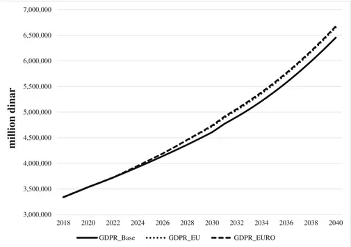
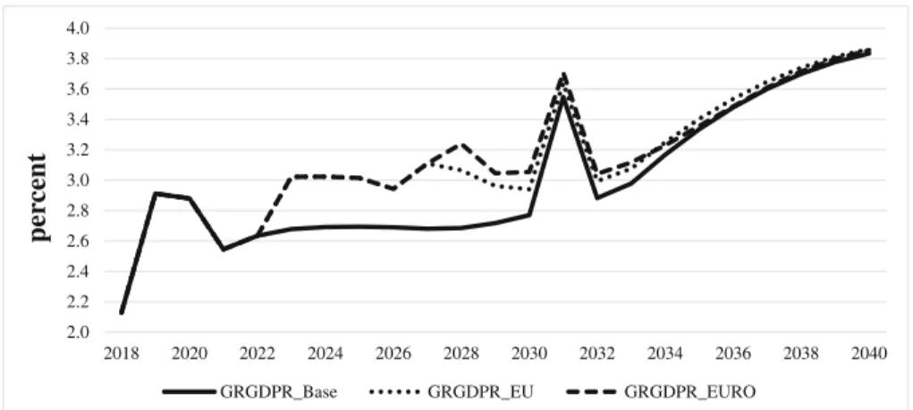
According to our simulation results, compared to the baseline, by 2040 real GDP is 3% higher in the scenario with EU accession, and 3.4% higher when Serbia also joins the Euro Area in 2023. The average real GDP growth rate amounts to 3.0% in the baseline scenario, 3.1% in the EU accession scenario, and 3.2% in the Euro Area accession scenario. The assumed higher TFP directly translates into an increase in potential GDP. Without any additional demand-side effects, this higher potential GDP leads to a reduction in capacity utilization, which reduces inflationary pressure.
3,000,000 3,500,000 4,000,000 4,500,000 5,000,000 5,500,000 6,000,000 6,500,000 7,000,000
2018 2020 2022 2024 2026 2028 2030 2032 2034 2036 2038 2040
million dinar
GDPR_Base GDPR_EU GDPR_EURO
Fig. 1 Real GDP. Source: Authors’own calculations and projections based on Eurostat (2018)
However, a lower capacity utilization also means less need for capacity- widening investment. On the other hand, we also assumed additional demand via exports, due to the reduction of trade barriers once Serbia has full access to the European Internal Market. This additional export demand has a positive multiplier effect on consumption and employment, and hence (via the acceler- ator effect) capital formation is also higher.
Net exports are affected positively in the EU accession scenario, which arises mainly from the assumed positive impacts on exports. In the Euro Area accession scenario, on the other hand, net exports deteriorate slightly. This is due to higher imports because of higher domestic demand. Furthermore, the increase in inflation induces a real appreciation of the Serbian currency.
2.0 2.2 2.4 2.6 2.8 3.0 3.2 3.4 3.6 3.8 4.0
2018 2020 2022 2024 2026 2028 2030 2032 2034 2036 2038 2040
percent
GRGDPR_Base GRGDPR_EU GRGDPR_EURO
Fig. 2 Real GDP growth rate. Source: Authors’own calculations and projections based on Eurostat (2018)
1,750,000 1,800,000 1,850,000 1,900,000 1,950,000 2,000,000
2018 2020 2022 2024 2026 2028 2030 2032 2034 2036 2038 2040
persons
EMP_Base EMP_EU EMP_EURO
Fig. 3 Employment. Source: Authors’own calculations and projections based on Eurostat (2018)
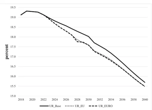
As mentioned, the labor market is influenced positively by the positive demand-side and supply-side impacts. By 2040, the number of employed persons is 0.3% higher both in the EU and the Euro Area accession scenarios as compared to the baseline. The unemployment rate drops to 15.5% in both scenarios com- pared to 15.7% in the baseline.
Due to higher demand and the assumed additional price increase in the Euro Area accession scenario, inflation is slightly higher in the two alternative
15.0 15.5 16.0 16.5 17.0 17.5 18.0 18.5 19.0 19.5
2018 2020 2022 2024 2026 2028 2030 2032 2034 2036 2038 2040
percent
UR_Base UR_EU UR_EURO
Fig. 4 Unemployment rate. Source: Authors’own calculations and projections based on Eurostat (2018)
1.5 2.0 2.5 3.0 3.5 4.0 4.5 5.0
2018 2020 2022 2024 2026 2028 2030 2032 2034 2036 2038 2040
percent
INFL_Base INFL_EU INFL_EURO
Fig. 5 Inflation rate. Source: Authors’own calculations and projections based on Eurostat (2018)
scenarios, despite the boost to potential GDP. However, this higher potential GDP restricts the additional inflation to less than 0.1 percentage points over the period 2023 (the assumed first year in which the macroeconomic effects of imminent EU accession materialize) to 2040.
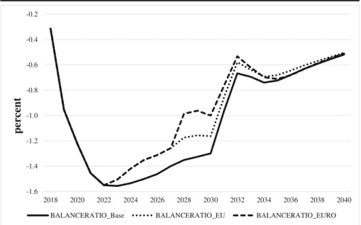
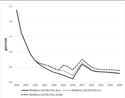
The EU and Euro Area accessions have positive effects on Serbia’s public finances, too. Without EU accession, in our simulations the debt-to-GDP ratio declines from 61.6% in 2017 to 25%. EU accession increases the decline to 23.5%, and Euro Area accession reduces the end-of-simulation-period debt ratio further to 23.0%. The increase in GDP causes higher tax revenues, and the improvement on the labor market leads to higher social security contributions by employees and employers and, correspondingly, lower expenditure on un- employment benefits. The higher revenues and reduced expenditures lead to a considerable improvement in the primary budget balance. The overall budget balance is additionally relieved by the reduced public debt, leading to lower interest outlays.
The interest rates remain on a high level in the baseline and the EU accession scenarios. The independent monetary policy pursued by the NSB thus remains relatively restrictive as a response to what is still a high rate of inflation. In the Euro Area scenario, monetary policy for Serbia is conducted by the European Central Bank. Hence, the interest rate in Serbia is substantially lower than in the case of an independent monetary policy. This effect could be observed in Euro Area countries on the Southern periphery of the EU after the composition of the Euro Area had been fixed. This drop in interest rates created additional private or public demand in Greece, Spain, and Portugal and similar effects cannot be excluded in the case of Serbia.
-1.6 -1.4 -1.2 -1.0 -0.8 -0.6 -0.4 -0.2
2018 2020 2022 2024 2026 2028 2030 2032 2034 2036 2038 2040
percent
BALANCERATIO_Base BALANCERATIO_EU BALANCERATIO_EURO
Fig. 6 Budget balance in relation to GDP. Source: Authors’own calculations and projections based on Eurostat (2018) and Serbian Ministry of Finance (2018)
Summary and Conclusions
By means of simulations with a macroeconometric model of the Serbian economy, this paper examines what macroeconomic effects can be expected from Serbia’s EU
20 25 30 35 40 45 50 55 60
2018 2020 2022 2024 2026 2028 2030 2032 2034 2036 2038 2040
percent
DEBTRATIO_Base DEBTRATIO_EU DEBTRATIO_EURO
Fig. 8 Public debt in relation to GDP. Source: Authors’own calculations and projections based on Eurostat (2018) and Serbian Ministry of Finance (2018)
0.0 0.5 1.0 1.5 2.0 2.5
2018 2020 2022 2024 2026 2028 2030 2032 2034 2036 2038 2040
percent
PRIMBALANCERATIO_Base PRIMBALANCERATIO_EU PRIMBALANCERATIO_EURO
Fig. 7 Primary budget balance in relation to GDP. Source: Authors’own calculations and projections based on Eurostat (2018) and Serbian Ministry of Finance (2018)
membership and from its membership of the Euro Area. Based on experiences with previous EU enlargement rounds, we assumed that Serbia will join the EU in 2025 and the Euro Area in 2028, and that EU accession will increase total factor productivity and exports. In addition, Euro Area accession will change its monetary policy regime since the European Central Bank will also conduct monetary policy for Serbia. The simula- tions with the macroeconometric model show that EU accession and the introduction of
2 3 4 5 6 7 8 9 10 11
2018 2020 2022 2024 2026 2028 2030 2032 2034 2036 2038 2040
percent
ILEND_Base ILEND_EU ILEND_EURO
Fig. 10 Long-term interest rate. Source: Authors’own calculations and projections based on Eurostat (2018) and Serbian Ministry of Finance (2018)
-14 -12 -10 -8 -6 -4 -2
2018 2020 2022 2024 2026 2028 2030 2032 2034 2036 2038 2040
percent
NEXPRATIO_Base NEXPRATIO_EU NEXPRATIO_EURO
Fig. 9 Net exports in relation to GDP. Source: Authors’own calculations and projections based on Eurostat (2018) and Serbian Ministry of Finance (2018)
the euro bring about higher real GDP and more employment, but also slightly higher inflation due to additional aggregate demand. Public finances are affected positively.
The benefits of joining the Euro Area are mainly due to supply side effects, namely.
productivity increases.
It should be admitted that our assumptions regarding the initial impacts of EU and Euro Area accession are to some extent arbitrary, but they are based on experiences in other countries. Furthermore, our model stresses the demand side, while the supply side comes into play mainly via potential GDP. Expectations are not forward looking in our model. Despite these limitations, the simulations show that positive macroeconomic effects can be expected for Serbia once it joins the EU and the Euro Area.
Acknowledgements Earlier versions of this paper were presented at the Allied Social Sciences Associations Meeting, Chicago, IL, January 6–8, 2017, the International Atlantic Economic Conference, London, March 14–17, 2018, and the Annual Meeting of the Austrian Economic Association, Vienna, May 11–12, 2018. Helpful comments by participants of these conferences, especially Ansgar Belke and Keshab Bhattarai, and an anonymous referee are gratefully acknowledged. The research reported in this paper was financially supported by the Austrian Science Fund FWF (project no. I 2764-G27).
Funding Information Open access funding provided by Austrian Science Fund (FWF).
Open AccessThis article is distributed under the terms of the Creative Commons Attribution 4.0 International License (http://creativecommons.org/licenses/by/4.0/), which permits unrestricted use, distribution, and repro- duction in any medium, provided you give appropriate credit to the original author(s) and the source, provide a link to the Creative Commons license, and indicate if changes were made.
References
Bohn, H. (1998). The behavior of U.S. public debt and deficits.Quarterly Journal of Economics, 113(3), 949–963.
Bower, U., & Turrini, A. (2010). EU accession: A road to fast-track convergence?Comparative Economic Studies, 52(2), 181–205.
Busch, B., Grömling, M., Ritzberger-Grünwald, D., Hishow, O. N., Hölscher, J., Kolev, S., & Zweynert, J.
(2014). EU-Osterweiterung: eine Bilanz nach zehn Jahren.Wirtschaftsdienst, 94(5), 311–334.
Cecchini, P., Catinat, M., & Jacquemin, A. (1988).The European challenge: 1992, the benefits of a single market. Aldershot: Wildwood House, UK.
European Commision (2018) European neighborhood policy and enlargement negotiations: Serbia. Available:
https://ec.europa.eu/neighbourhood-enlargement/countries/detailed-country-information/serbia_en. 3 Dec 2018.
Eurostat (2018). Database. Available:https://ec.europa.eu/eurostat/data/database. 3 Dec 2018.
Lejour, A., Mervar, A., & Verweij, G. (2009). The economic effects of Croatia’s accession to the European Union.Eastern European Economics, 47(6), 60–83.
Mastrobuoni, G. (2004), The effects of the Euro-Conversion on prices and price perceptions.CEPS Working Paper101, September 2004. Brussels.
Organization for Economic Cooperation and Development (2001),Measuring capital. Organization for Economic Cooperation and Development Manual: Measurement of Capital Stocks, Consumption of Fixed Capital and Capital Services. Paris.
Pataki, Z. (2014).The cost of non-Europe in the single market.“Cecchini revisited”. An overview of the potential economic gains from further completion of the European single market. Brussels: EPRS– European Parliamentary Research Service http://www.europarl.europa.eu/RegData/etudes/STUD/2014 /510981/EPRS_STU%282014%29510981_REV1_EN.pdf. 3 Dec 2018.
Roberts, B.V. (2002), An analysis of Macedonian economic growth during 1997–2001.Republic of Macedonia, Ministry of Finance, Bulletin11–12/2002.
Serbian Ministry of Finance (2018). Macroeconomic Survey. Available:http://www.mfin.gov.rs/pages/issue.
php?id=3. 3 Dec 2018.
Serbian Statistical Office (2018). STAT database. Available: http://data.stat.gov.rs/?caller=
SDDB&languageCode=en-US#. 3 Dec 2018.
Vetter, S. (2013).The single European market 20 years on. Achievements, unfulfilled expectations & further potential. Frankfurt/Main: DB Research, EU Monitorhttps://www.dbresearch.com/PROD/RPS_EN- PROD/PROD0000000000444504/The_Single_European_Market_20_years_on%3A_Achievemen.PDF.
Weyerstrass, K., & Grozea-Helmenstein, D. (2013). A Macroeconometric Model for Serbia.International Advances in Economic Research, 19(2), 85–106.
Weyerstrass, K., & Neck, R. (2008). Macroeconomic effects of Slovenia’s integration in the euro area.
Empirica, 35, 391–403.
Zagorchev, A., Vasconcellos, G., & Bae, Y. (2011). Financial development, technology, growth and perfor- mance: Evidence from the accession to the EU.Journal of International Financial Markets, Institutions and Money, 21(5), 743–759.
Publisher’s Note Springer Nature remains neutral with regard to jurisdictional claims in published maps and institutional affiliations.