Wage discrimination against immigrants in Austria?

Supported by the Austrian Science Funds

Wage discrimination against immigrants in Austria?

by

Helmut HOFER Gerlinde TITELBACH Rudolf WINTER-EBMER*)

Working Paper No. 1407 June 2014

The Austrian Center for Labor Economics and the Analysis of the Welfare State

JKU Linz

Department of Economics Altenberger Strasse 69 4040 Linz, Austria www.labornrn.at

Corresponding author: rudolf.winterebmer@jku.at

Wage discrimination against immigrants in Austria?

Helmut Hofer

* Gerlinde Titelbach*

Rudolf Winter-Ebmer * **

Draft

This version: June 2014

Abstract: This paper analyses wage discrimination against immigrants in Austria using combined information from the labor force surveys and administrative social security data.

We find that immigrants experience a wage disadvantage of 15 percentage points compared to natives. However, a substantial part of the wage gap can be explained by differences in human capital endowment and job position. Decomposition methods using quantile regressions show larger discrimination in the upper part of the wage distribution. Moreover, we do not find any evidence for wage assimilation of immigrants in Austria.

* Institute for Advanced Studies Vienna, ** University of Linz

§ Corresponding author; Institute for Advanced Studies Vienna, Stumpergasse 56, A 1060

Vienna, email:

Thomas Liebig and the participants of the NOeG conference 2014 in Vienna for comments

and Birgit Wögerbauer and Johannes Schachner for research assistance.

1. Introduction

In Austria the share of immigrants in the population amounts to 19 percent in 2012 and is one of the largest in the OECD. In international comparison general labor market integration outcomes are not unfavorable (see e.g. Krause and Liebig 2011). However, empirical evidence shows disadvantages of immigrants with respect to employment, unemployment, job offers and position in the occupational hierarchy (see e.g. Huber 2010, Liebig and Krause 2011, Titelbach et al. 2013, Weichselbaumer 2013). In this paper, we will analyze wage differentials between immigrants and natives for Austria in a systematic way, using matched data from labor force surveys and administrative social security data.

One can define discrimination as unequal treatment that disfavors immigrants against natives. Taste-based and statistical discrimination has been distinguished in the economic literature (see Becker 1957, Arrow, 1973). While the former relates to unequal treatment due to preferences of economic agents, the latter derives unequal treatment from incomplete knowledge about the true productivity of workers which may lead to stereotyping behavior. In the following empirical analysis, we will contrast two basic principles of equal treatment:

“equal pay for equal endowments” versus “equal pay for equal work”. The first principle implements a broader definition of discrimination: wage differentials which cannot be explained by typical (observable) productivity characteristics, like education and training are labelled discrimination. The second principle implements a definition of discrimination which is narrower. Wage differentials due to different job characteristics, like industry, occupation or hierarchical position in a firm are taken out: only inexplicable wage differentials for natives and immigrants in the same jobs are defined as discrimination. This definition does not take into account how the workers got this job.

For Austria – with the exception of Grandner and Gstach (2014) - almost no research exists on this topic due to data limitations. In our empirical analysis we first use Oaxaca-Blinder decomposition techniques to determine wage differentials at the mean of the distribution.

Moreover, we apply quantile decomposition techniques to analyze the heterogeneity of discrimination and human capital effects across the wage distribution. Finally, we test the wage assimilation hypothesis for Austria.

In other countries, wage discrimination against immigrants has been extensively analyzed in

recent years (see e.g. OECD 2013 for a review). The early wage assimilation hypothesis by

Barry Chiswick (1978) for the United States suggests that immigrants close the initial wage

gap with natives within 10 to 15 years, and then they may overtake due to the very high

wage growth. The original results by Chiswick of an overtaking of the immigrants are based

on cross-sectional data. Longitudinal data, where immigrants could be tracked over time,

show indeed a catch up, but not an overtaking of immigrants anymore in relation to

individuals who were born in the United States (Borjas 1985).

In European countries, wage differentials between natives and immigrants are less frequently analyzed. For the United Kingdom, Elliot and Lindley (2008) show a wage differential of about 16 percent among white British men and non-white immigrants, this differential cannot be explained by differences in productivity. Bell (1997) finds no wage disadvantage for white immigrants. However, black immigrants who spent a greater part of their career abroad face wage disadvantages. Dustmann et al. (2010) again demonstrate that immigrants from OECD countries have higher wages as natives in the UK.

For Germany Lehmer and Ludsteck (2011) show that most immigrant groups have 20 percent lower wages than native Germans. The differences are largest for Poles and smallest for the Spanish. The result of an Oaxaca-Blinder decomposition shows that approximately half of the differential is explained by differences in productivity. Controlling for occupation lowers the unexplained part by 20-30 percent. Hirsch and Jahn (2012) show that about 14 to 17 percentage points of this 20 percentage point wage differential can be explained by observable productivity characteristics (including occupation). Beblo et al.

(2012) report a difference in wages between Germans and foreign workers of approximately 15.5 percent for the period 1996 to 2007. They find strong evidence that foreign workers are employed disproportionately often in low-wage firms. Controlling for these firm effects reduces the wage differential to 10.6 percent of which about 8 percentage points can be explained by observable productivity characteristics such as education, work experience and tenure. Moreover, Licht and Steiner (1993) find no evidence for the assimilation hypothesis in Germany.

For Denmark, Nielsen et al. (2004) find a higher wage differential between foreigners and natives for men than for women. Males from Turkey, Africa and Pakistan earn 22 percent, 23 percent, and 26 percent, respectively, less than natives. The wage penalty for female immigrants from these countries amounts to 17 percent. In an Oaxaca-Blinder decomposition including the standard human capital variables, occupation and hierarchical job position as productivity measures, nearly the full differential is explained for males. For women approximately one third of the differential remains unexplained. In the case of Spain, Canal-Dominguez et al. (2008) find wage differentials of nearly 40% of which three quarters can be explained by differences in productivity (including job position).

Several studies analyze the gender wage differential in Austria empirically (see e.g. Winter-

Ebmer and Zweimüller, 1994, Böheim et al. 2013); however, empirical evidence on wage

differentials by nationality or migration status is very scarce. In a first study, Grandner and

Gstach (2014) use the EU-SILC data for the analysis of wage discrimination between

immigrants and natives for Austria. They report a wage penalty in the range of 15 to 25

percent. They use counterfactual densities to decompose the wage differential and report a

discrimination component ranging from 5 to 20 percentage points. The discrimination

component follows a marked U-shape over the income distribution reaching a maximum at

around the 8th decile. While Grandner and Gstach (2014) use comparable EU survey data

from a relatively small sample, we can profit from the combination of comprehensive administrative with high-quality labor force data. We consider wage differentials between natives and immigrants for male and female separately to avoid problems with gender wage differentials.

The remainder of the paper is organized as follows. The next section presents the methods we use to analyze wage discrimination. Section 3 deals with a description of our data source and presents basic information on differences in characteristics between immigrants and natives. Section 4 discusses the econometric results. The final section concludes.

2. Methods to measure discrimination

In this paper wage differentials between natives and immigrants are analyzed by decomposition methods (see Fortin et al., 2011 for a general overview). The Oaxaca-Blinder (OB) approach decomposes the wage gap of natives and immigrants in a component due to differences in productivity-related characteristics and a so-called residual term ("discrimination component").

This method splits up the average wage gap. This mean decomposition result is only representative if the coefficients do not vary across the wage distribution. We use a quantile regression framework to investigate differential effects across the wage distribution. Finally, we apply simple regression analysis to test the wage assimilation hypothesis for Austria.

The Oaxaca-Blinder method is used to decompose the average wage differential between natives (I) and foreigners (A) in a productivity-related difference (E) and a so-called discrimination component (U).

ln − = +

The starting point is the so called Mincer wage equation which is estimated for each of the two groups separately. The log hourly wage is a linear function of a variety of individual and firm level characteristics, e. g. education, work experience, job tenure, firm size, industry.

The coefficient vector ß reflects the price of the individual characteristics, such as the wage effect of an additional year of schooling.

ln = ß +

and

groups. It follows that

-

. Let’s assume that a non-discriminatory coefficient vector ß* exists. Then the average wage gap can be decomposed in the following way:

1 See Weichselbaumer and Winter-Ebmer (2005) for the rhetoric in the use of “discrimination” or “unexplained residual” in gender research.

ln − =

-

-ß

+

The first term E = -

the different endowments of the two groups with productivity-related characteristics. U =

-ß

+

represents the unexplained residual or the discrimination component. It should be noted that this part also includes all unobservable differences between the groups.

The decomposition used requires an estimate of the non-discriminatory wage structure

We assume that the wage structure of the natives is non-discriminatory

. Substituting ß as an estimate of ß

ln − =

-

-ß

Again, the first factor represents the portion of the wage gap that is due to differences in endowments, while the second part represents the unexplained residual.

After the analysis of the mean wage gap we use quantile regressions (QR) to analyze the wage differentials at different points of the wage distribution. QR models specify the q

conditional quantile of the log wage distribution as a linear function of the explanatory variables (see Koenker and Hallock 2001 for an introduction):

ln = ß + , i=I, A

with

and E[

]=0. In contrast to OLS regressions, QR do not have the property that the mean value of the dependent variable and the means of the explanatory variables lie on the regression line. As a consequence, a simple OB decomposition is not possible.

Following the literature (e.g. Böheim et al. 2013, Lehmer and Ludsteck 2011) we use the method of Melly (2006) to estimate counterfactual wage distributions.

In a first step, the conditional wage distribution is estimated by QR. In a second step, the conditional distribution over the range of the explanatory variables is integrated out, thereby obtaining an estimator for the unconditional wage distribution. Based on the distribution of characteristics of the foreigners and the coefficients that result from the estimate with the data of the natives, we obtain the counterfactual distribution that would result if foreigners would achieve the same returns on their productivity-relevant characteristics as natives. For each quantile the wage differential between native and foreigners can be decomposed into two parts. The first (explained) part is due to differences in the distribution of productivity-

2 Due to the relatively small number of immigrants, it is less sensible to assume the foreigner’s wage structure to be the non-discriminatory one; therefore, the usual index number problem in decomposition analysis does not apply here.

relevant characteristics. The second component (discrimination) reflects differences in the returns to characteristics.

The validity of such a decomposition depends on the selection of explanatory variables in the wage function. If one selects too many control variables, discrimination could be underestimated. This can be illustrated with an example from the gender discrimination research. If there is a so-called glass ceiling and women are not promoted to top positions, then a regression with a control variable “occupational rank” would underestimate discrimination as this variable would represent an endogenous variable. If one assumes instead a narrower concept of discrimination, i.e. one considers only wage differentials between persons with the same human capital and similar occupational ranks, than the control variable is justified. Lehmer and Ludsteck (2011) discuss this problem with respect to occupation dummies. If the selection into occupations depends only on productive characteristics, which may not be visible to the researcher but are, in fact, observable by the employer (e. g. imperfect transferability of human capital acquired in foreign countries, insufficient languages skills), occupational dummies are justified. On the other hand if assignment to occupations is governed by discriminatory preferences of employers, the inclusion of occupational dummies masks discrimination.

To provide bounds according to these two views, we use two different specifications of the wage function. Specification I is based on a broader definition of discrimination. In this specification education, work experience, job tenure, employment days in the Austrian labor market within the last 5 years, firm size, marital status, number of children, level of urbanization and region are included in the wage equation as explanatory variables. We include also, in addition to that, dummies for industry, occupation (vertical segregation), hierarchical position (horizontal segregation) and blue-white-collar (specification II). The equations are estimated separately for men and women, respectively, using OLS.

These two specifications ideally correspond to two different concepts of discrimination.

Specification II is based on the principle of "equal pay for equal work": Ideally, we want to control for the type of job, the occupational hierarchy etc.: this concept makes a comparison between two employees (of different nationalities) at the same job. It does not matter how these two people came into this job. Note however, that the allocation of jobs, career advancement etc. may already have been characterized by unequal treatment.

The measure of overall discrimination in the labor market could therefore have been underestimated. Specification I defines discrimination as "equal pay for equal endowments":

as only productivity features are used as explanatory factors, but no features of the job.

This level of discrimination may represent an overestimation of discrimination because some

3 “Ideally” here means that in the above mentioned case not all job-relevant characteristics and not all productivity- relevant characteristics may be measurable.

productivity-relevant characteristics of the workers may not be exactly measured and they could possibly affect wages through job allocation. These two issues of the measurement of discrimination provide a common area of discussion which occurs in similar ways in the gender pay gap discussion. In this field the glass ceiling with respect to promotions and the choice or assignment of women to typical low-paid women's jobs are major research topics.

3. Data

We combine the Austrian micro-census (labor force survey) with data from social security records. The data set was matched at the individual level. For reasons of data protection, the matching was done by Statistics Austria and the econometric estimations were carried out in the safe center of Statistics Austria. The merged data contain human capital variables, such as education and experience, workplace characteristics and complete working history since 1988. The sample size corresponds to the number of observations in the micro-census.

The Austrian micro-census is a quarterly panel survey which collects information on private households. It is representative of the Austrian population and contains information of about 80,000 individuals per year. Every quarter a fifth of the sample is renewed. The micro-census served as the central data source for the study. Since valid statements for different migrant groups require an adequate sample size, the micro-censuses of the years 2008 to 2010 were pooled and the data of the second quarter was used. The micro-census was used to get information on personal (sex, age, nationality, migration background) and labor market characteristics (occupation, current employment status, working hours, industry, and job position). The indicator for the job position depends on skill requirements and occupation.

We differentiate between the following job

leading manager in large firms). The data from the micro-census are supplemented with information from the labor market database which is based on social security registers.

The data about income of the Federation of Austrian Social Insurance (contribution bases)

are used for the mean wage gap analysis because information is available for 2008-2010. In

addition to the income data, employment days within a year, job tenure and firm size have

been taken from the labor market data base. Furthermore, an indicator of the employment

days in Austria within the last five years was constructed. Based on the annual income in the

respective firm, the associated employment days and the standard working hours according

to the micro-census, gross hourly wages were calculated as an indicator of the salary. The

analysis of the effects across the wage distribution is undertaken with income data from the

micro-census. The income information of the micro census 2009 and 2010 is based on wage

tax records data (Baierl et al. 2011) and is not censored at the maximum contribution celling.

4

Net hourly wages are used as the dependent variable.

Our estimation sample consists of full-time employed workers aged 20 to 55 who were active in the years 2008-2010 in the private sector of the Austrian economy. For the respective employment in the second quarter of each year, the hourly wage was calculated and deflated to prices of 2006. Only workers who were employed at least 270 days in their companies were included.

Migration status is based on the concept of migration background. People with a migration background are defined as persons whose parents were both born abroad. This migrant group can be divided in the first generation (country of birth abroad) and the second generation (country of birth is Austria). The use of this concept has some advantages compared to a definition by nationality. For example, a change of citizenship does not cause a selection problem and for immigrants of second generation the problems of unobservable characteristics (language capabilities, quality of school education abroad) do not matter.

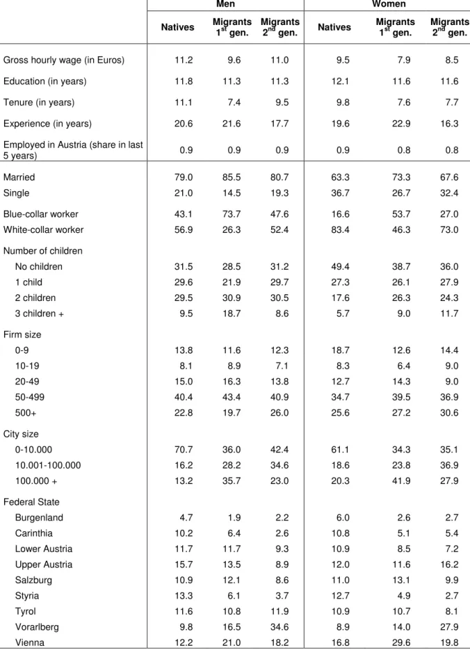
In Table 1Table 1 summary statistics for natives and immigrants are shown. Hourly wages of immigrants are about 15 percent lower than those of the natives. However, it also becomes apparent that natives and immigrants differ in their productivity-related characteristics. One of the most important determinants of wages is the amount of formal schooling. Immigrants have on average half a year less years of education. Also job tenure is considerably shorter.

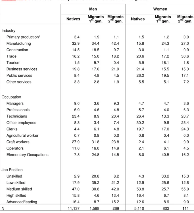
Immigrants live more often in large cities and in the provinces of Vienna and Vorarlberg. With respect to industry the share of immigrants is above average in manufacturing and in the tourism sector. Significant differences are also apparent in occupation and job position. On average, immigrants have a higher probability to work in low wage occupations and less favorable job positions. Three quarters of male and slightly more than half of female immigrants are blue-collar workers. For Austrians, the corresponding proportions are 43 percent and 17 percent, respectively. One out of five (three) migrant males (females) work in elementary occupations. For Austrians this applies only to three to four percent. These data show considerable heterogeneity between natives and immigrants with respect to human capital and job positions.

4 Only in the highest 1% of income, the actual values are replaced by the median of these groups (Baierl et al .2011).

5 Following Böheim et al. (2013b) this limitation was used to eliminate short-term employment or seasonal employment episodes. Foreigners are found with a higher probability in less stable or in seasonal jobs. We redid the analysis with a minimum employment period of 60 days: approximately the same results arise.

Table 1: Descriptive statistics: natives and immigrants

Men Women

Natives Migrants 1^st gen.

Migrants

2^nd gen. Natives Migrants 1^st gen.

Migrants 2^nd gen.

Gross hourly wage (in Euros) 11.2 9.6 11.0 9.5 7.9 8.5

Education (in years) 11.8 11.3 11.3 12.1 11.6 11.6

Tenure (in years) 11.1 7.4 9.5 9.8 7.6 7.7

Experience (in years) 20.6 21.6 17.7 19.6 22.9 16.3

Employed in Austria (share in last

5 years) 0.9 0.9 0.9 0.9 0.8 0.8

Married 79.0 85.5 80.7 63.3 73.3 67.6

Single 21.0 14.5 19.3 36.7 26.7 32.4

Blue-collar worker 43.1 73.7 47.6 16.6 53.7 27.0

White-collar worker 56.9 26.3 52.4 83.4 46.3 73.0

Number of children

No children 31.5 28.5 31.2 49.4 38.7 36.0

1 child 29.6 21.9 29.7 27.3 26.1 27.9

2 children 29.5 30.9 30.5 17.6 26.3 24.3

3 children + 9.5 18.7 8.6 5.7 9.0 11.7

Firm size

0-9 13.8 11.6 12.3 18.7 12.6 14.4

10-19 8.1 8.9 7.1 8.3 6.4 9.0

20-49 15.0 16.3 13.8 12.7 14.3 9.0

50-499 40.4 43.4 40.9 34.7 39.5 36.9

500+ 22.8 19.7 26.0 25.6 27.2 30.6

City size

0-10.000 70.7 36.0 42.4 61.1 34.3 35.1

10.001-100.000 16.2 28.2 34.6 18.6 23.8 36.9

100.000 + 13.2 35.7 23.0 20.3 41.9 27.9

Federal State

Burgenland 4.7 1.9 2.2 6.0 2.6 2.7

Carinthia 10.2 6.4 2.6 10.8 5.1 5.4

Lower Austria 11.7 11.7 9.3 10.9 8.5 7.2

Upper Austria 15.7 13.5 8.9 12.0 11.6 16.2

Salzburg 10.9 12.1 8.6 11.0 13.1 9.9

Styria 13.3 6.1 3.7 12.7 4.9 2.7

Tyrol 11.6 10.8 11.9 10.9 10.7 8.1

Vorarlberg 9.8 16.5 34.6 8.9 14.0 27.9

Vienna 12.2 21.0 18.2 16.8 29.6 19.8

Table 1Table 1 continued: Descriptive statistics: natives and immigrants

Men Women

Natives Migrants 1^st gen.

Migrants

2^nd gen. Natives Migrants 1^st gen.

Migrants 2^nd gen.

Industry

Primary production* 3.4 1.9 1.1 1.5 1.2 0.0

Manufacturing 32.9 34.4 42.4 15.8 24.3 27.0

Construction 14.5 18.5 9.7 3.0 1.1 0.9

Trade 16.2 15.0 18.2 20.6 17.2 30.6

Tourism 1.5 5.7 0.4 5.9 16.1 1.8

Business services 19.8 17.0 21.9 21.4 15.5 15.3

Public services 8.4 4.8 4.5 26.2 19.5 17.1

Other services 3.3 2.8 1.9 5.5 5.1 7.2

Occupation

Managers 9.0 3.6 9.3 4.7 4.7 3.6

Professionals 6.9 4.6 4.8 5.7 4.0 6.3

Technicians 23.4 8.9 20.4 26.4 13.3 20.7

Office employees 8.8 3.4 7.4 30.2 9.9 23.4

Clerks 4.4 6.1 4.8 19.7 17.0 24.3

Agricultural worker 0.7 0.8 0.0 0.8 0.4 0.0

Craft workers 27.9 31.8 23.8 2.4 4.1 0.9

Operators 11.0 16.0 14.9 2.1 6.1 4.5

Elementary Occupations 7.8 24.8 14.5 8.0 40.5 16.2

Job Position

Unskilled 2.9 20.8 8.2 4.3 33.2 15.3

Low skilled 17.9 35.2 21.2 12.9 25.6 12.6

Medium skilled 47.0 30.8 42.0 53.8 25.7 55.0

High skilled 15.8 4.6 13.4 16.4 6.7 8.1

Advanced/leading 16.4 8.7 15.2 12.6 8.9 9.0

N 11,137 1,598 269 5,110 802 111

Source: Micro-census 2008-2010, AMDB

* Primary production includes agriculture, forestry, mining and the energy sector

4. Results

4.1. Wage differentials at the mean

The descriptive evidence revealed marked differences in the endowments of natives and immigrants. We use the Oaxaca-Blinder decomposition to explore the native-migrant wage gap. (Table 4Table 4 and

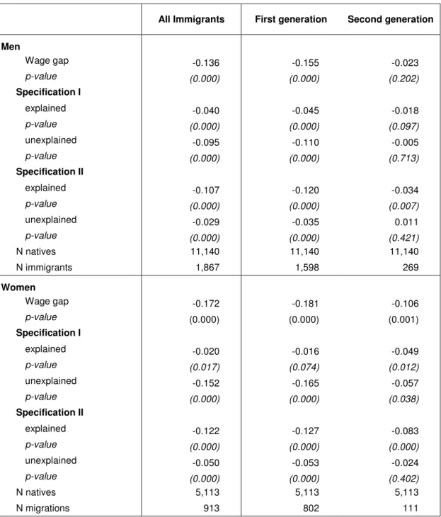
equation.) According to Table 2Table 2, the raw wage gap between natives and immigrants amounts to 13.6 log percentage points for men and 17.2 log percentage points for women, respectively. The analysis shows that differences in human capital (education and experience) contribute significantly to the observed wage gap. Differences in human capital alone explain 30 percent of the wage gap for males, for women the share is slightly above 11 percent

specification I). A detailed decomposition reveals that the unexplained gap is mainly related to lower returns to schooling and especially work experience of immigrants.

Controlling for occupation and in particular job position (specification II) reduces the unexplained wage gap even further. The discrimination component falls to 3 (5) log percentage points for males (females).

We find very different results for first and second generation immigrants. For the first generation the raw wage differential amounts to approximately 17 log percentage points. The raw wage differential for the immigrants of the second generation is considerably smaller (males 2, females 11 log percentage points). First generation immigrants are endowed with less human capital (schooling, tenure). These differences explain approximately one quarter of the raw wage differential of males, for females the share is only one tenth. Differences in occupation and in particular job position are even more important as human capital variables. According to specification II the unexplained part of the wage gap falls to 3.5 (males) and 5.3 log percentage points (females), respectively.

For male immigrants of second generation we only find a very small raw wage differential, which is not statistically significant. This small gap can be explained by the less favorable human capital endowment. Overall, there is no evidence for discrimination of male immigrants of second generation. The situation for female immigrants of second generation is different: their raw wage gap amounts to 10.6 log percentage points. Approximately one half of the raw wage differential can be explained by differences in human capital endowment (schooling, experience). Controlling for occupation and job position reduces the unexplained wage gap to 2.4 log percentage points. Note that the discrimination component is not statistically significant, which may also be due to the small sample size for migrants.

The very low returns to experience for female second generation immigrants are striking.

Table 2: Oaxaca-Blinder decomposition

All Immigrants First generation Second generation Men

Wage gap -0.136 -0.155 -0.023

p-value (0.000) (0.000) (0.202)

Specification I

explained -0.040 -0.045 -0.018

p-value (0.000) (0.000) (0.097)

unexplained -0.095 -0.110 -0.005

p-value (0.000) (0.000) (0.713)

Specification II

explained -0.107 -0.120 -0.034

p-value (0.000) (0.000) (0.007)

unexplained -0.029 -0.035 0.011

p-value (0.000) (0.000) (0.421)

N natives 11,140 11,140 11,140

N immigrants 1,867 1,598 269

Women

Wage gap -0.172 -0.181 -0.106

p-value (0.000) (0.000) (0.001)

Specification I

explained -0.020 -0.016 -0.049

p-value (0.017) (0.074) (0.012)

unexplained -0.152 -0.165 -0.057

p-value (0.000) (0.000) (0.038)

Specification II

explained -0.122 -0.127 -0.083

p-value (0.000) (0.000) (0.000)

unexplained -0.050 -0.053 -0.024

p-value (0.000) (0.000) (0.402)

N natives 5,113 5,113 5,113

N migrations 913 802 111

Note: P-values for a test of the null hypothesis that the coefficient is not different from zero are presented in parentheses.

A comparison of the returns to schooling between the first and second generation is

interesting. The returns are comparatively low for the first generation immigrants. In contrast,

male second generation immigrants earn the same returns as natives. The returns among

women of the second generation remain slightly behind natives. This evidence indicates

problems in the transferability of human capital which was acquired abroad.

4.2. Decompositions for the entire wage distribution

The Oaxaca-Blinder approach splits up the wage gap at the average level. As unequal treatment may happen differently at different job or wage levels, we now turn to decompositions along the entire wage distribution using quantile regressions. We use net hourly wages as dependent variable and restrict the estimation period to 2009 and 2010.

Due to the small number of cases a splitting up of the group of immigrants into first and second generation is not possible.

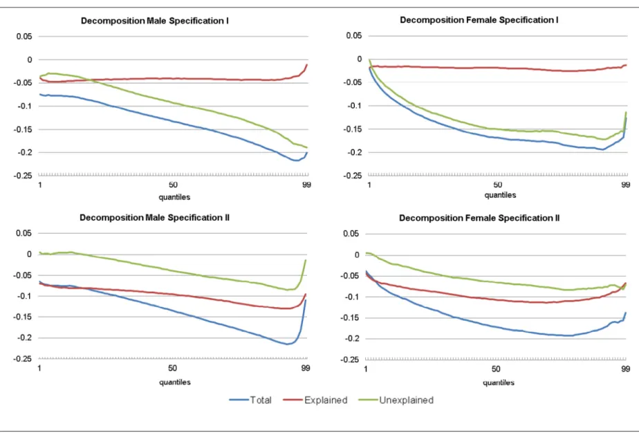
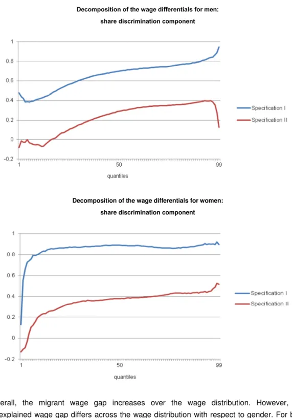
Figure 1 shows the decomposition of wage differentials measured in log points, whereas Figure 2 concentrates on the discrimination components only. The discrimination component is shown here as share of total wage differential at the respective quantil of the distribution.

99 quantile regressions were estimated, separately for each quantile of the wage distribution.

It turns out that the wage disadvantage of immigrants’ increases with the wage level (see the blue graph "differential" in Figure 1).

At the bottom of the wage distribution it amounts to 8 log percentage points for males and then rises steadily to almost 22 log percentage points.

Only in the top decile it falls slightly. The increase in the wage gap is even steeper for females. For the 25th percentile it amounts to 13 log percentage points and then rises up to 19 percentage points for the 90th percentile. In the highest income range, the wage gap is slightly smaller. Overall we find a considerable wage disadvantage for immigrants, in particular in the middle and upper part of the wage distribution.

For men, the discrimination component increases with income (see Figure 2). Accordingly, 40 percent of the wage gap can be explained by productivity-related characteristics at the 10th percentile of the wage distribution (specification I). The discrimination share climbs up to around 90 percent at the 90th percentile. In the top decile the endowment differences in the productivity-related characteristics are smaller, so that almost the total wage differential must be attributed to discrimination. According to specification II no discrimination can be found at the bottom of the wage distribution (up to the 20th percentile), then the discrimination proportion rises to 40 percent (95th percentile).

For females we find a somewhat different picture (specification I). Only at the very bottom of the wage distribution the unexplained wage gap is small, but then it rises steeply and is already around 85 percent at the 20th percentile. Afterwards the discrimination share remains constant. Specification II results in a very similar picture, however with a smaller discrimination component. In the lower third of the wage distribution the discrimination component increases markedly, than it flattens out.

6 At the edge of the distribution (at the 1st, 2nd, or at the 98th, 99th percentile) the results should not be interpreted, because typically there is a low number of observations.

Figure 1: Decomposition of the wage differential

Figure 2: Discrimination component

Decomposition of the wage differentials for men:

share discrimination component

Decomposition of the wage differentials for women:

share discrimination component

Overall, the migrant wage gap increases over the wage distribution. However, the

unexplained wage gap differs across the wage distribution with respect to gender. For both

groups and in the lowest part of the wage distribution, discrimination against immigrants is

very low or even absent. For females the unexplained wage gap increases strongly with the

wage. For men the discrimination component rises continuously but the level remains below

that of women until the fourth quintile of the wage distribution.

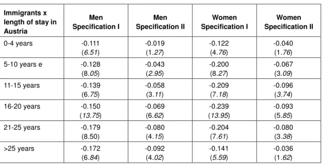
4.3. Test of the assimilation hypothesis for Austria

Finally, we turn to the question of wage assimilation in Austria. Especially in the American literature (Chiswick 1978, Borjas 1985) there is a discussion whether and when immigrants are able to close the wage gap with natives. We investigate this question for natives and first generation immigrants who migrated at the age of 15 or later. We differentiate between immigrants according to their length of stay in Austria. We estimate a similar wage function as above with the difference that now natives and immigrants are considered together, and use six dummies with respect to the length of stay times migration status (0-4 years, 5-10 years, 11-15 years, 16-20 years, 21-25 years and over 25 years).

Table 3Table 3 shows no evidence for wage assimilation in Austria. Irrespective of the length

of stay, wage differentials are the same: most of the coefficients - which one can compare vertically in each column - are not statistically significantly different from each other. We only find very minor evidence for wage assimilation for females living more than 25 years in Austria. On the contrary we find no significant wage gaps for immigrants who immigrated recently (women specification II).

Table 3: Assimilation hypothesis Immigrants x

length of stay in Austria

Men Specification I

Men Specification II

Women Specification I

Women Specification II

0-4 years -0.111

(6.51)

-0.019 (1.27)

-0.122 (4.76)

-0.040 (1.76) 5-10 years e -0.128

(8.05)

-0.043 (2.95)

-0.200 (8.27)

-0.067 (3.09) 11-15 years -0.139

(6.75)

-0.058 (3.11)

-0.209 (7.18)

-0.096 (3.74)

16-20 years -0.150

(13.75)

-0.069 (6.62)

-0.239 (13.95)

-0.093 (5.85)

21-25 years -0.179

(8.50)

-0.080 (4.15)

-0.204 (7.61)

-0.080 (3.38)

>25 years -0.172 (6.84)

-0.092 (4.02)

-0.141 (5.59)

-0.036 (1.62)

Note: dependent variable: gross hourly wage (log); Specification I and II without share of employment in Austria in the last 5 years; italic numbers in brackets: t-statistics

Analogous to the discussion between Borjas (1985) and Chiswick (1978) for the United

States the problem of our analyses is that we cannot distinguish between assimilation and

cohort effects because only cross-section data is available. The variable length of stay in

Austria measures in addition to the length of stay also all the specific characteristics of the

arrival cohort who came to Austria exactly x years ago. If the unobserved characteristics of

these cohorts have changed over time this could also explain the estimated non-assimilation.

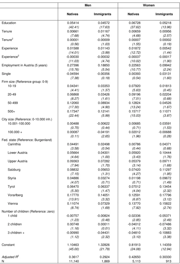
Table 4: Wage equation men and women: natives vs. immigrants, specification I

Men Women

Natives Immigrants Natives Immigrants

Education 0.05414 0.04572 0.06728 0.05218

(42.41) (17.63) (37.62) (13.96)

Tenure 0.00661 0.01167 0.00659 0.00956

(7.68) (4.74) (4.68) (2.57)

Tenure² 0.00001 -0.00009 0.00007 0.00002

(0.56) (1.03) (1.55) (0.19)

Experience 0.01588 0.01143 0.01872 0.00542

(14.01) (3.99) (12.72) (1.44)

Experience² -0.00030 -0.00032 -0.00037 -0.00017

(11.03) (4.74) (10.02) (1.90)

Employment in Austria (5 years) 0.27396 0.18850 0.22563 0.09942

(15.76) (5.54) (10.77) (2.24)

Single -0.04594 -0.00356 0.00393 0.03131

(7.38) (0.19) (0.54) (1.60)

Firm size (Reference group: 0-9)

10-19 0.04341 0.03353 0.07920 0.01813

(4.41) (1.37) (5.63) (0.45)

20-49 0.06868 0.03426 0.09196 0.02204

(8.27) (1.61) (7.51) (0.68)

50-499 0.12060 0.08934 0.12824 0.04526

(17.30) (4.90) (13.24) (1.67)

500+ 0.17347 0.12141 0.15717 0.11071

(22.44) (5.99) (15.03) (3.87)

City size (Reference: 0-10.000 inh.)

10.001-100.000 0.00488 -0.00622 0.00685 0.03591

(0.75) (0.44) (0.71) (1.53)

100.000 + 0.00087 -0.04191 0.02012 -0.00688

(0.11) (2.65) (1.96) (0.28)

Fed. state (Reference: Burgenland)

Carinthia 0.04491 0.02498 0.00786 0.04371

(3.58) (0.54) (0.44) (0.68)

Lower Austria 0.05664 0.04301 0.05920 0.10444

(4.64) (1.00) (3.43) (1.76)

Upper Austria 0.09363 0.07282 0.05379 0.09711

(7.94) (1.70) (3.14) (1.68)

Salzburg 0.08832 0.05653 0.07420 0.11297

(7.15) (1.31) (4.27) (1.95)

Styria 0.04886 0.03274 0.01198 0.09672

(4.07) (0.71) (0.71) (1.49)

Tyrol 0.06470 0.06337 0.07012 0.13454

(5.30) (1.47) (4.04) (2.32)

Vorarlberg 0.17770 0.14051 0.12591 0.17796

(13.91) (3.32) (6.87) (3.12)

Vienna 0.11074 0.07329 0.13770 0.15822

(8.74) (1.69) (7.92) (2.74)

Number of children (Reference: zero)

1 child -0.00757 -0.00824 -0.02336 -0.05371

(1.23) (0.48) (2.85) (2.49)

2 children 0.00748 0.00011 -0.04012 -0.07486

(1.16) (0.01) (4.11) (3.32)

3 children + -0.00990 -0.04431 -0.04810 -0.10883

(1.12) (2.32) (3.10) (3.38)

Constant 1.10463 1.32826 0.81913 1.14359

(45.00) (21.79) (24.08) (12.94)

Adjusted R² 0.3617 0.2924 0.42650 0.30330

N 11,140 1,869 5,113 913

Note: dependent variable: gross hourly wage (log, italic numbers in brackets t-statistics

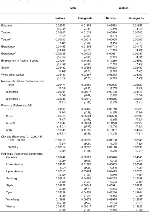
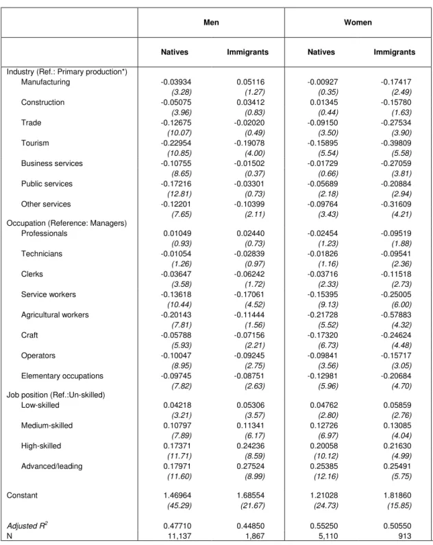
Table 5: Wage equation: natives vs. immigrants, specification II

Men Women

Natives Immigrants Natives Immigrants

Education 0.02553 0.01358 0.03522 0.01957

(16.02) (4.46) (17.01) (4.94)

Tenure 0.00607 0.01023 0.00520 0.00700

(7.77) (4.66) (4.17) (2.21)

Tenure² -0.00003 -0.00011 0.00005 0.00003

(1.12) (1.34) (1.29) (0.31)

Experience 0.01495 0.01206 0.01743 0.01473

(14.43) (4.72) (13.28) (4.49)

Experience² -0.00025 -0.00029 -0.00031 -0.00032

(10.25) (4.96) (9.67) (4.32)

Employment in Austria (5 years) 0.24261 0.14989 0.19260 0.05560

(15.26) (4.92) (10.33) (1.45)

Single -0.03492 -0.00256 0.01203 0.02450

(6.18) (0.16) (1.86) (1.47)

White-collar worker 0.08140 0.03687 0.06313 0.04269

(12.35) (2.16) (4.93) (1.49)

Number of children (Reference: zero)

1 child -0.00471 -0.00859 -0.02005 -0.05827

(0.85) (0.56) (2.76) (3.15)

2 children 0.00981 0.00917 -0.03438 -0.04816

(1.68) (0.62) (3.97) (2.50)

3 children + 0.00246 -0.02810 -0.04515 -0.06661

(0.31) (1.65) (3.27) (2.41)

Firm size (Reference: 0-9)

10-19 0.04408 0.05160 0.05748 0.02728

(4.94) (2.38) (4.59) (0.80)

20-49 0.06918 0.05024 0.07558 0.02590

(9.17) (2.66) (6.92) (0.92)

50-499 0.11542 0.08954 0.11278 0.00522

(18.01) (5.47) (12.74) (0.22)

500+ 0.16940 0.11799 0.13957 0.04652

(23.51) (6.39) (14.36) (1.81)

City size (Reference: 0-10.000 inh.)

10.001-100.000 -0.00318 -0.00299 -0.01108 0.03646

(0.54) (0.24) (1.29) (1.82)

100.000 + -0.00314 -0.02656 0.01118 0.00090

(0.45) (1.88) (1.23) (0.04)

Fed. state (Reference: Burgenland)

Carinthia 0.03742 -0.00229 0.00678 0.04640

(3.29) (0.06) (0.43) (0.84)

Lower Austria 0.04508 0.01383 0.03835 0.06342

(4.07) (0.36) (2.51) (1.25)

Upper Austria 0.07315 0.03924 0.04423 0.07671

(6.82) (1.03) (2.91) (1.55)

Salzburg 0.06212 0.04863 0.04263 0.12149

(5.53) (1.27) (2.76) (2.45)

Styria 0.03822 0.00542 0.00991 0.08237

(3.50) (0.13) (0.66) (1.47)

Tyrol 0.05529 0.04758 0.06286 0.13941

(4.99) (1.25) (4.09) (2.80)

Vorarlberg 0.12668 0.09671 0.09975 0.12287

(10.88) (2.57) (6.13) (2.51)

Vienna 0.08052 0.05017 0.09367 0.13627

(6.99) (1.30) (6.05) (2.76)

Table 5Table 5 continued: Wage equation: natives vs. immigrants, specification II

Men Women

Natives Immigrants Natives Immigrants

Industry (Ref.: Primary production*)

Manufacturing -0.03934 0.05116 -0.00927 -0.17417

(3.28) (1.27) (0.35) (2.49)

Construction -0.05075 0.03412 0.01345 -0.15780

(3.96) (0.83) (0.44) (1.63)

Trade -0.12675 -0.02020 -0.09150 -0.27534

(10.07) (0.49) (3.50) (3.90)

Tourism -0.22954 -0.19078 -0.15895 -0.39809

(10.85) (4.00) (5.54) (5.58)

Business services -0.10755 -0.01502 -0.01729 -0.27059

(8.65) (0.37) (0.66) (3.81)

Public services -0.17216 -0.03301 -0.05689 -0.20884

(12.81) (0.73) (2.18) (2.94)

Other services -0.12201 -0.10399 -0.09764 -0.31609

(7.65) (2.11) (3.43) (4.21)

Occupation (Reference: Managers)

Professionals 0.01049 0.02440 -0.02454 -0.09519

(0.93) (0.73) (1.23) (1.88)

Technicians -0.01054 -0.02839 -0.01826 -0.09541

(1.26) (0.97) (1.16) (2.36)

Clerks -0.03647 -0.06242 -0.03716 -0.11518

(3.58) (1.72) (2.33) (2.73)

Service workers -0.13618 -0.17061 -0.15395 -0.25005

(10.44) (4.52) (9.13) (6.00)

Agricultural workers -0.20143 -0.11444 -0.21728 -0.57883

(7.81) (1.56) (5.52) (4.32)

Craft -0.05788 -0.07156 -0.17320 -0.24624

(5.93) (2.21) (6.73) (4.48)

Operators -0.10047 -0.09245 -0.09841 -0.15717

(8.95) (2.75) (3.56) (3.05)

Elementary occupations -0.09745 -0.08751 -0.12981 -0.20684

(7.82) (2.63) (5.96) (4.70)

Job position (Ref.:Un-skilled)

Low-skilled 0.04218 0.05306 0.04762 0.05859

(3.21) (3.57) (2.80) (2.76)

Medium-skilled 0.10797 0.11341 0.12726 0.13085

(7.89) (6.17) (6.97) (4.04)

High-skilled 0.17371 0.24236 0.20058 0.21630

(11.71) (8.59) (10.12) (4.99)

Advanced/leading 0.17971 0.27524 0.25385 0.25491

(11.60) (8.99) (12.16) (5.75)

Constant 1.46964 1.68554 1.21028 1.81860

(45.29) (21.67) (24.73) (15.85)

Adjusted R² 0.47710 0.44850 0.55250 0.50550

N 11,137 1,867 5,110 913

Note: dependent variable: gross hourly wage (log), italic numbers in brackets: t-statistics

*primary production = agriculture, forestry, mining and the energy sector

5. Conclusions

In this paper we analyze wage discrimination against immigrants in Austria. We match data from the micro-census and social security records to provide new evidence for Austria. We find a raw wage gap of immigrants of approximately 15 log percentage points. Results from Oaxaca/Blinder decomposition show that 10 to 30 percent of this wage gap can be explained by differences in endowment of human capital. Controlling for occupation and in particular for job position reduces the discrimination component considerably. In this case, the unexplained part of the wage gap amounts to 3 to 5 log percentage points. Overall, the unexplained wage gap of immigrants is small, according to the principle `equal pay for equal work´. However, one should note that controlling for occupation and job position is justified only if the selection with respect to occupation and job position depends on productivity relevant characteristics only (e.g. transferability of human capital acquired abroad, language skills). Otherwise the degree of discrimination is clearly underestimated. Overall our results for Austria are in line with evidence from other European countries, e.g. Germany. In contrast to the study of Grandner and Gstach (2014) we find a lower raw wage differential for Austria, especially in the lower part of the income distribution. According to our results wage discrimination against immigrants is somewhat lower, in particular when we control for job characteristics. In accordance with Grandner and Gstach we find that discrimination is stronger in the upper part of the wage distribution. Furthermore, the unexplained gender wage gap reported by Böheim et al. (2013) for Austria is considerably higher as our estimates for the wage gap between natives and immigrants.

We differentiate between first and second generation immigrants. Our results show no evidence for discrimination of second generation immigrants. Furthermore, we use quantile regressions to investigate the wage gap across the wage distribution. We find evidence for higher wage gaps and more discrimination at the upper part of the income distribution.

Overall we find some evidence showing problems for immigrants to transfer their human capital acquired abroad. Immigrants are very often found in unfavorable job positions. The data show no evidence for wage assimilation. Measures for a better integration of foreign workers in the Austrian labor market are desirable. While our data are so far the best available in Austria for such a purpose, some caveats remain: We have no information on language skills which could be an important factor for the success on the labor market. In future research we plan to investigate discrimination for special migrant groups (e.g.

immigrants from (ex-) Yugoslavia, Turkey).

References

Arrow K. J. (1973): The theory of discrimination, discrimination in labor markets, Princeton University Press, 3-33.

Baierl, A., Gumprecht, D. und N. Gumprecht (2011): Monatliches Nettoeinkommen im Mikrozensus - Konzept, Statistische Nachrichten, 596-612.

Beblo, M., Ohlert, C. and E. Wolf (2012): Ethnic wage inequality within German establishments: Empirical evidence based on linked employer-employee data, Harriet Taylor Mill-Institut für Ökonomie und Geschlechterforschung, Berlin, Discussion Paper 19.

Becker, G. S. (1957): The economics of discrimination, Chicago: University of Chicago Press.

Bell, B. (1997): The performance of immigrants in the UK: Evidence from the GHS, The Economic Journal, 333-344.

Blinder, A. S. (1973): Wage discrimination: Reduced form and structural estimates, Journal of Human Resources, 8, 436-455.

Böheim, R., Himpele, K., Mahringer, H. and C. Zulehner (2013): The distribution of the gender pay gap in Austria: evidence from matched employer-employee data and tax records, Journal for Labour Market Research, 46, 19-34.

Borjas, G. (1985): Assimilation, changes in cohort quality, and earnings of immigrants, Journal of Labor Economics, 3(4), 463-489.

Canal-Domínguez, J. F. and C. Rodríguez-Gutiérrez (2008): Analysis of wage differences between native and immigrant workers in Spain, Spanish Economic Review, 10, 109–134.

Chiswick, B. R. (1978): The effect of Americanization on the earnings of foreign-born, Journal of Political Economy, 86(5), 897-921.

Dustmann, C., Gltiz, A. and T. Vogel (2010): Employment, wages, and the economic cycle:

Differences between immigrants and natives, European Economic Review, 54(1), 1-17.

Elliot, R. and Lindley, J. (2008): Immigrant wage differentials, ethnicity and occupational segregation, Journal of the Royal Statistical Society, 171(3), 645-671.

Fortin, N., T. Lemieux, and S. Firpo, (2011); Decomposition methods in economics, in Ashenfelter O., Layard, R. and D. Card (eds.), Handbook of Labor Economics, Vol. 4A, 1- 102.

Grandner, T., and D. Gstach (2014): Decomposing wage discrimination in Germany and Austria with counterfactual densities, forthcoming in Empirica.

Hirsch, B. and E. Jahn (2012): Is there monopsonistic discrimination against immigrants?

First evidence from linked employer-employee data. LASER Discussion paper, 59.

Huber, P. (2010): Die Arbeitsmarktintegration von Migrantinnen und Migranten in Österreich, WIFO Working Paper 365, Wien.

Jahn B. (2008): The Blinder-Oaxaca decomposition for linear regression models. The Stata Journal, 8(4), 453-479.

Koenker, R. and K. F. Hallock (2001): Quantile regression, Journal of Economic Perspectives, 15(4), 143-156.

Krause, K. and T. Liebig (2011): The labour market integration of immigrants and their children in Austria. OECD Social, Employment and Migration Working Papers 127.

Directorate for Employment, Labour and Social Affairs: OECD Publishing.

Lehmer, F. and J. Ludsteck (2011): The immigrant wage gap in Germany: Are East Europeans worse off? International Migration Review, 4, 872-906.

Licht, G. and V. Steiner (1994): Assimilation, labor market experience, and earnings profiles of temporary and permanent immigrant workers in Germany, International Journal of Applied Economic, 8(2), 130-156.

Melly, B. (2006): Estimation of counterfactual distributions using quantile regression, mimeo.

Nielsen, H. S., Rosholm, N., Smith, N. and L. Husted (2004): Qualifications, discrimination or assimilation: an extended framework for analysing immigrant wage gaps, Empirical Economics, 29, 855-883.

Oaxaca, R. (1973): Male-female wage differentials in urban labor markets, International Economic Review, 14, 693-709.

OECD (2013): Discrimination against immigrants – measurement, incidence and policy instruments, in: International Migrant Outlook 2013, OECD, 191-230.

Titelbach, G., Davoine, T., Hofer, H., Schuster, P. und M. Steiner (2013): Potentiale durch die Integration von Migrant/innen in Arbeitsmarkt und Bildung, Studie im Auftrag des Integrationsfonds, IHS, Wien.

Weichselbaumer, D. (2013): Correspondence Testing (Kapitel 3), in: Hofer, H., Titelbach, G., Weichselbaumer, D. und R. Winter-Ebmer, Diskriminierung vom MigrantInnen am österreichischen Arbeitsmarkt, Studie im Auftrag des BMASK, IHS, Wien.

Weichselbaumer, D. and R. Winter-Ebmer (2005): Rhetoric in Economic Research: The Case of Gender Wage Differentials, Industrial Relations 45/3.

Winter-Ebmer, R. and J. Zweimüller (1994): Gender Wage Differentials in Private and Public

Sector Jobs, Journal of Population Economics, 7(3); 271-285.