Evaluating Theories of the Income Dynamics: A Probabilistic Approach

(1)

IHS Economics Series Working Paper 61

February 1999

Evaluating Theories of the Income Dynamics: A Probabilistic Approach

Robert Aebi

Klaus Neusser

Peter Steiner

(2)

Impressum Author(s):

Robert Aebi, Klaus Neusser, Peter Steiner Title:

Evaluating Theories of the Income Dynamics: A Probabilistic Approach ISSN: Unspecified

1999 Institut für Höhere Studien - Institute for Advanced Studies (IHS) Josefstädter Straße 39, A-1080 Wien

E-Mail: o ce@ihs.ac.atﬃ Web: ww w .ihs.ac. a t

All IHS Working Papers are available online: http://irihs. ihs. ac.at/view/ihs_series/

This paper is available for download without charge at:

https://irihs.ihs.ac.at/id/eprint/1136/

(3)

Institut für Höhere Studien (IHS), Wien Institute for Advanced Studies, Vienna

Reihe Ökonomie / Economics Series No. 61

Evaluating Theories of the Income Dynamics:

A Probabilistic Approach

Robert Aebi, Klaus Neusser, Peter Steiner

(4)

Evaluating Theories of the Income Dynamics: A Probabilistic Approach

Robert Aebi, Klaus Neusser, Peter Steiner

Reihe Ökonomie / Economics Series No. 61

February 1999

Robert Aebi

Institute for mathematical Statistic University of Berne

Sidlerstrasse 5

Ch-3012 Berne, Switzerland Phone: +41/31/631-8818 E-mail: aebu@math-stat.unibe.ch

Klaus Neusser

Department of Economics University of Berne Gesellschaftsstrasse 49 CH-3012 Berne, Switzerland Phone: +41/31/631-4776 Fax: +41/31/631-3992

E-mail: klaus.neusser@vwi.unibe.ch

Peter Steiner

Department of Economics University of Berne Gesellschaftsstrasse 49 CH-3012 Berne, Switzerland Phone: +41/31/631-4780 Fax: +41/31/631-3992 E-mail: peter.steiner@vwi.unibe.ch

Institut für Höhere Studien (IHS), Wien

Institute for Advanced Studies, Vienna

(5)

The Institute for Advanced Studies in Vienna is an independent center of postgraduate training and research in the social sciences. The Economics Series presents research done at the Economics Department of the Institute for Advanced Studies. Department members, guests, visitors, and other researchers are invited to contribute and to submit manuscripts to the editors. All papers are subjected to an internal refereeing process.

Editorial Main Editor:

Robert M. Kunst (Econometrics) Associate Editors:

Walter Fisher (Macroeconomics) Klaus Ritzberger (Microeconomics)

(6)

Abstract

The paper proposes an approach to evaluate hypotheses about transition dynamics when only the distributions at two points in time are observed. Using the principle of statistical mechanics, we show how to adjust in the “most probable” way a hypothesis so that it becomes compatible with the observed distributions. This adjustment procedure also allows to test hypotheses in a statistical sense. The test is based on the relative entropy and is equivalent to a likelihood ratio test. We apply our approach to compare the dynamics of the income distribution between men and women in the U.S. using PSID data.

Keywords

Transition matrices, large deviation, relative entropy, income dynamics

JEL Classifications

J30, C10

(7)

1. Introduction 1

2. Concepts and Theoretical Background 2

Probabilistic Model 2

Probability of Income History Matrices 4 Maximization and Adjusted Dynamics 4 Test Statistic 7

3. Comparing the Income Dynamics of Women and Men 8

The Data 8

4. Empirical Results 9

5. Conclusion 11

References 12

(8)

(9)

I H S — Aebi, Neusser, Steiner / Evaluating Theories of the Income Dynamics — 1

1. Introduction

Recent years have witnessed a growing interest in the analysis of the evolution of an income distribution over time. This renewed interest arose from two different vividly debated issues. The first issue relates to the so-called convergence hypothesis. This hypothesis asserts that differences across countries in per capita income are transitory, controlling for technology, preferences and population growth rates. As has been forcefully pointed out by Quah (1996), the cross-country growth equation initially advocated by Barro and Sala-i-Martin (1992) suffers from severe deficiencies which lead to unreliable conclusions. Instead, Quah (1996) suggests to ”model explicitly the dynamics of the entire cross-country distribution of incomes”. The second issue relates to the recently observed increase in income inequality in some countries (notably the U.S. and the U.K.). The reasons for this rise are widely debated and have brought the income distribution ”in from the cold” (Atkinson 1997; Gottschalk 1997). In order to assess this rise in inequality it is important to develop a notion of mobility within the income distribution. This, however, requires to model again the dynamics of the entire distribution.

Although this renewed interest comes from two quite different economic traditions and concerns, the analysis of the dynamics of the distribution uses similar tools. In both strands of literature, the evolution of the income distribution is analyzed in terms of a transition probability matrix (or a stochastic kernel in case of a continuous state space) estimated from panel surveys. The convergence hypothesis can then be assessed by computing the stationary distribution or passage times associated with the transition matrix;¹ mobility is assessed by computing some scalar mobility measure from the transition matrix.²

Although these applications produce interesting insights, they are purely descriptive in nature.

They lack a probabilistic foundation and do not formally test or evaluate theories of income dynamics formulated in terms of the transition matrix. We think that this is a serious drawback which hinders further progress in these fields. The purpose of our paper is therefore to provide the methodological foundations to the testing and evaluation of theories of income dynamics.

Although we expose our views by investigating a concrete problem, we think that our approach can be fruitfully extended to related issues.

The problem we want to analyze is the following. Suppose we are in a situation where the distribution of income is observed at two points in time and where no information on the incomes of the members in the population is available. We may think of having at our disposal a repeated cross-section at two points in time. Suppose further that we want to evaluate some hypothesis about the transition dynamics. This hypothesis may have been derived from

1 Durlauf and Quah (1998) provide extensive references and a critical assessment of the literature.

2 For a theoretical discussion see Shorrocks (1978). Schluter (1998) and Trede (1998) provide examples of empirical applications.

(10)

2 — Aebi, Neusser, Steiner / Evaluating Theories of the Income Dynamics — I H S

theoretical considerations or from samples drawn from another population. Besides the methodological issues, this concrete problem is of considerable practical interest because individual income histories are often not recorded. Although by construction no information on the income of any member in the two periods is available, we will show that it is nevertheless possible to draw meaningful statistical inferences on the transition dynamics under these circumstances. Moreover, we will show how to adapt our hypothesis ”optimally” given the information presented by observed distributions.

It turns out that the above problem is equivalent to the problem of fitting the cell probabilities of a contingency table when the marginal probabilities are known and fixed. This question has been treated in the statistical literature by Deming and Stephan (1940) and Ireland and Kullback (1968) among others. These authors also propose an algorithm known as iterative proportional fitting procedure (IPFP) to solve this problem in practice. Recently, Aebi (1996, 1997) gives a probabilistic framework in terms of ”large deviations” for contingency tables. He shows how to compute “most probable” adjustments of observed contingency tables to prescribed marginals based on the fundamental hypothesis of statistical mechanics. In this paper we follow his interpretation and use a large deviation principle to operationalize the meaning of “most probable”.

We do not only develop the theoretical concepts, but we also illustrate our approach by a practical example. In particular, we compare the income dynamics of men and women in the U.S. using the PSID data set. These data encompass more information than we actually need because the PSID data trace individual incomes over time. This additional information will, however, allows us to assess and document the validity of our approach.

2. Concepts and Theoretical Background

Probabilistic Model

Suppose that for a population consisting of a large number of N independent individuals we observe the distribution of income at two points in time t and s with t < s. As our exposition relies on a finite state space, we take a finite partition I = {Ii}i=1,...,k of R⁺ and assume that income is distributed in the two time periods according to the discrete probability distributions qt = (q1t, . . ., qkt)´ and qs = (q1s, . . ., qks)´ defined on I, i.e. qit is the probability that income in period t falls in the i-th interval.

If we were actually in a position to trace the income of each individual in the population, we could count how many persons starting in income class i in period t arrive in income class j in period s. Denote these numbers by Γij and arrange them in a k×k matrix

(11)

Γ = (Γij)i,j=1,...,k

We call this matrix the income history matrix. Note that the income history matrix is unobserved. We only know that it must be compatible with the observed income distributions at time t and s, qt and qs. Thus if nobody gets lost or is joining in going from period t to s, each person starting in income class i must end up in some income class j, likewise each person ending up in income class j must have started in some income class i. When the number of persons N is large, these restrictions on the income history matrix can be stated as follows:

(1)

k j 1 Nq

k i 1 Nq

js k

1 i

ij it k

1 j

ij

≤

= Γ

≤

= Γ

∑

=

If we denote by ι the k-vector of ones, these restrictions can be written more compactly as

(1')

s t

Nq Nq

= ι Γ′

= ι

Γ

Because Σi qit = 1 and Σj qjs = 1, the above conditions impose 2k – 2 independent restrictions on Γ, referred to as continuity restrictions or initial and terminal conditions.

The theory or hypothesis about the dynamics of the income distribution between the two periods t and s is formulated in terms of a two-dimensional joint probability distribution. This can be done either directly or, more conveniently, indirectly via a transition probability matrix.³ If we denote by P = (pij)i,j=1,...,k the transition matrix representing our hypothesis, the elements pij

are just the probabilities of moving to income class j given that the individual was in income class i. For any given income distribution, π = (π1, . . ., πk)´, in period t, πi pij i s then the probability that an individual is in income class i in period t and in class j in period s. The two-dimensional joint probability is then given by the matrix (πi pij)i,j=1,...,k = diag(π) P.

With these preliminaries we can state formally the problem we seek to address. Find the income history matrix Γ which would have the maximum likelihood of being observed under our maintained hypothesis, diag(π) P, subject to the continuity restrictions (1). We solve this problem in two steps. We compute first the probability of observing a particular income history

3 Champernowne (1953) was the first one to view the income distribution as the equilibrium outcome of a Markov process specified by a transition matrix. He presented conditions on the transition matrix such that the ergodic distribution satisfies Pareto´s law. Later Wagner (1978), and more recently Conlisk (1990) and Dardanoni (1994), discussed alternative hypotheses about the form of the transition matrix.

(12)

matrix and then solve the underlying maximization problem. The analysis is, however, not straightforward because our hypothesis does not satisfy the continuity restrictions. The law of large numbers then implies that, viewed from the perspective of our hypothesis, the probability of every income history matrix goes to zero as N tends to infinity. We resolve this indeterminacy by relying on a large deviation principle, i.e. we seek the income history matrix whose probability goes to zero at the slowest rate.

Probability of Income History Matrices

Assuming that the evolution of individual incomes is independent from each other, the probability that a particular history of N persons belongs to the income history matrix Γ is

∏

^k₌

( ) ^π

^Γ

1 j , i

ij i

p

ij

The next step is to compute the number of possible histories which belong to a given income history matrix. This corresponds to the number of arrangements of N distinguishable individuals as subsets of Γij persons. It is obtained by an elementary combinatorial argument:

∏

∑ ∑ ∑

∑

=

−

=

−

=

−

=

Γ

 =

 





 







Γ

− Γ

−

 







 





 Γ

Γ

−

 

  Γ

Γ

− Γ

 −



 



 Γ

Γ

 −



 





Γ

^k

1 j , i kk ij

1 k

1 i

1 k

1 j

kj 1

k

1 j

ij

21 k

1 j

j 1 13

12 11 12

11

!

! N N

N N N

N L L

The income history matrix Γ is therefore realized with probability PN(Γ) given by

(2)

( ) _∏ ( ) _∏ ( )

∏

⁼

Γ

=

Γ

=

Γ

= π Γ π

=

Γ

^k

1 j ,

i ij

ij i k

1 j , i

ij k i

1 j ,

i ij

N

!

! p N p

!

! P N

ij ij

Maximization and Adjusted Dynamics

There are infinitely many income history matrices which are compatible with the continuity restrictions (1). To determine the income history matrix Γ uniquely, we adopt the fundamental hypothesis of statistical mechanics to the evolution of incomes: an observation at the macroscopic level is realized in the limit of infinitely many individuals by that microscopic ensemble which has maximal probability (i.e. is “most probable”) given the observation. This principle means that we want to choose the income history matrix which has the highest probability of being realized, viewed from the perspective of our conjecture, and which satisfies

(13)

the continuity conditions. Chapter I in Ellis (1985) provides an insightful introduction to the concepts we will use subsequently.

As explained previously, the law of large numbers implies that every income history matrix has probability zero as N tends to infinity, PN(Γ) → 0 as N → ∞, because Γ satisfies the continuity restrictions whereas our conjecture diag(π)P does not. We can nevertheless obtain a unique solution to our maximization problem if we interpret ”most probable” as ”vanishing at the slowest rate”. This is a so-called large deviation principle. The rate at which the probability (2) goes to zero is given by the limit of (1/N) log PN(Γ). Using Stirling’s formula for large factorials,⁴ this limit is

(3)

^log ^P ( ) ^H ( ^diag ( ) ^P )

N lim 1

_N

N

Γ = − γ π

∞

→

where γ = (γij) denotes the matrix Γ/N = (Γij/N). The function H(γ|diag(π)P) is known as the relative entropy or Kullback-Leibler divergence of the two-dimensional distribution γ with respect to diag(π)P and is defined as

(4)

( ( ) ) ∑

=

 





 



 π γ γ

= π

γ

^k

1 j ,

i i ij

ij

log p

P diag H

where it is understood that 0 log(0) equals 0 and that γij log(γij/(πipij)) equals infinity if πipij equals 0 and γij ≠ 0. The function H(.|diag(π)P) is also called the rate function because PN(Γ) decays to zero exponentially fast at a rate given by (4). It can be shown that H(.|diag(π)P) is a nonnegative and convex function. Moreover, H(.|diag(π)P) equals zero if and only if γ = diag(π)P.

Thus H(.|diag(π)P) attains its infinum at the unique measure γ = diag(π)P. These properties suggest to interpret the relative entropy H(γ|diag(π)P) as a distance or a measure of discrepancy from the distribution diag(π)P to the distribution γ. The relative entropy does, however, not define a metric because it is not symmetric in its arguments and because it violates the triangular inequality.⁵

The relative entropy can be interpreted as a measure of the probability of observing a given income history matrix viewed from the standpoint of our conjecture. The principle of statistical mechanics then advises us to take the ”most probable” income history matrix subject to the

4 Stirling´s formula is

(

x

)

x

1 x e 2

! x

x  π +ε



 



= ^withε^x→ 0 as x →∞.

5 Further properties of the relative entropy and a deeper discussion of its interpretation can be found among others in Kullback (1959), Ellis (1985), and Hillman (1996).

(14)

continuity restrictions. This amounts to minimize H(γ|diag(π)P) over all two-dimensional distributions γ subject to the continuity restrictions (1). In the words of the statistics literature, we have to find the minimum discrimination information under the hypothesis diag(π)P (Kullback 1959, 37). The solution is called the minimum discriminant information adjustment of diag(π)P (Haberman 1984). The Lagrangian L for this optimization problem is

(5)

∑ ∑ ∑ ∑ ∑

= =

=

 

 



 γ − λ

 −

 

 γ − λ

 −







 



 π γ γ

=

^k

1 j

k

1 i

js ij js k

1 i

k

1 j

it ij it k

1 j ,

i i ij

ij

q q

log p L

where λit and λjs are the 2k Lagrangian multipliers associated with the constraints (1).

Differentiating (5) with respect to γij and setting the derivative equal to zero yields the “most probable” income history probability density matrix denoted by G = (gij):

(6) gij = φit πipij φjs

where φit equals exp(λit) and φjs equals exp(λjs-1). In matrix notation the above relation becomes

(6´) G = Φt diag(π)P Φs

where Φt and Φs denote diag((φ1t,...,φkt)) and diag((φ1s,...,φks)).

In the theory of quantum mechanics the φ´s are known as Schrödinger multipliers. They indicate how to adjust ”in the most probable” way the two-dimensional density diag(π) P, representing our conjecture about income dynamics, to satisfy the continuity restrictions (1).

The Schrödinger multipliers adjust the probabilities of our hypothesis (πipij) downward if φit × φjs

is smaller than one and upward if φit × φjs is larger than one. The matrix (φitφjs)i,j=1,...,k may therefore reveal patterns of adjustment and indicate to us the ”region” of our hypothesis which produce the ”large systematic errors”.

The Schrödinger multipliers are found after differentiating L with respect to the Lagrangian multipliers (λit) and setting the derivatives equal to zero. The resulting equation system is the so-called Schrödinger system:

(7)

js js k

1 i

ij i it

it k

1 j

js ij i it

q p

=

 φ



 



 φ π

= φ π φ

∑

=

(15)

This equation system shows that the Schrödinger multipliers are unique only up to a multiplicative constant. In the following we normalize the φ´s such that φ1t equals φ1s. Moreover and most importantly, the Schrödinger multipliers have a kind of ”separability property” because the φit´s depend only on the distribution at time t whereas the φis´s depend only on the distribution at the time s. Thus the relative size of φt and φs indicates whether the adjustment is primarily due to the initial or to the terminal restriction.

In empirical applications it is often more convenient to deal with transition probabilities instead of two-dimensional densities. We can reformulate the adjustment equation (6´) in terms of the

”most probable” transition matrix Q = (qij). Given the initial distribution qt, the elements of the two-dimensional density and of the transition matrix are related by gij = qij qit. The elements of Q are therefore obtained from P as follows

(8)

s 1 s

k 1

j ij js

js ij k

1

j ij js

i it

js ij i it it

ij ij

~ P Q

p p p

p q

q g

Φ Φ

=

φ

= φ φ π

φ

φ π

= φ

=

−

=

∑

where

Φ ~

s

= diag ( _∑

^k_j=₁

p

ij

φ

js

)

. Note that Q satisfies the definition of a transition matrix, i.e.

qij ≥ 0 and

q

_ij

j k

∑

=¹

⁼ ¹

for all i. Moreover, Q is obtained from P only through the Schrödinger multipliers φjs related to the end restrictions.

Test Statistic

From a statistical point of view, we do not only want to know how to best adjust our hypothesis, but also if these adjustments are significant. For this purpose, it is convenient to interpret the computation of G as estimating the cell probabilities of a k×k contingency table for which the marginal probabilities, in our case qt and qs, are given. This problem was first treated by Deming and Stephan (1940) who also suggest an iterative procedure, known as iterative proportional fitting procedure (IPFP), to solve the Schrödinger system (7). Taking the φjs equal to one as starting values, the φit can be computed from the first part of (7). Inserting these values in the second part of (7), new values for φis are obtained. These can then be used to update the φit. This procedure is then repeated until convergence is achieved.⁶ Having found the Schrödinger multipliers, it is straightforward to compute G and Q using equations (6) and (8). It can be shown that this procedure converges geometrically fast, generates best asymptotically normal (BAN) estimates and is equivalent to maximum likelihood estimates (Smith 1947;

Ireland and Kullback 1968). In addition, these latter authors show that the statistic 2N times

6 The procedure assumes that πipij > 0. Clearly, if πipij = 0, gij = 0.

(16)

the relative entropy function is asymptotically distributed as chi-squared and can thus be used to test our conjecture, i.e.

(9)

2 N H ( G diag ( ) π P ) ~ χ

²2k₋2

According to Ireland and Kullback (1968), the degree of freedom, 2k-2, is given by the difference between the degrees of freedom in the unrestricted model, k²-1, and in the restricted model, k²-2k+1. Therefore the degree of freedom corresponds to the number of restrictions imposed by the continuity restrictions (1).⁷

3. Comparing the Income Dynamics of Women and Men

The Data

We illustrate our approach by asking whether the observed distributions of women’s income are compatible with the income dynamics estimated for men over the same period. To answer this question we use data from the panel study of income dynamics (PSID).⁸ The "1968-1993 individual file" records, among other information, the annual income of 53'013 individuals from 1967 through 1992. We divided the sample period into 5-year intervals and extracted the variables "total annual work hours", "type of income", "total annual income" and "age of individual". Due to a change in data collection, we retrieved in 1992 the variable "total annual labor income" instead of "total annual income”. In order to save space, this paper focuses on the last 5-year interval (1987 to 1992).⁹

To obtain sensible and meaningful results, we used only a subset of the whole sample. In particular, we applied to the following restrictions:

• We focus on labor income only.

• Individuals have to be at least of age 20 in the starting year and at most of age 60 in final year of the 5-year intervals.

• We only look at fully employed individuals. People with less than 1800 hours worked per year are eliminated from the sample.

7 The same result can be obtained by observing that (5) is just the Neyman-Pearson statistic subject to the restrictions (1) (see Billingsley 1961, chapter 5).

8 URL: http://www.isr.umich.edu/src/psid/maindata.html; file 68_93ind.zip.

9 The other 5-year intervals give similar conclusions and are available upon request.

(17)

• Despite these restrictions some extreme outliers remained in the sample.¹⁰ To eliminate them, we require a minimum annual income of 1´000 USD in 1967. This minimum is inflated in subsequent years by the growth rate of the mean income.

After processing the restrictions mentioned above, the male data set contained 1'180 and the female data set 935 individuals. To construct transition matrices and two-dimensional discrete distributions, we had to choose partitions for the starting and the final year. Setting k arbitrarily equal to 10, we chose the income interval bounds in both years such that the number of men is equally distributed among the 10 cells. Thus the i-th interval is the interval with bounds given by the (i–1)-th and i-th percentile of men´s income distribution.

The female incomes are distributed according to the partitions defined for men. This procedure resulted in the marginal densities of the beginning and the final year for women. In case several female incomes happen to be exactly equal to some bound of the partition, the incomes are equally split between the two adjacent cells of the marginal density.

The income distribution of women in the two years 1987 and 1992 is plotted in figure 1.

Remember that the probability for men is equal to 0.1 in both years by construction. This figure reveals that the mode of the density shifted from the first to the second income class. In addition, more women are now in the upper income classes. These two simple observations suggest that women’s income distribution has obviously changed over these five years. The question we want to address is whether these changes can be explained by the income dynamics estimated for men.

4. Empirical Results

The income dynamics for men is represented by the two-dimensional density matrix in table 1 and the corresponding transition matrix in table 2. The cell probabilities are estimated by the method of maximum likelihood which just equals the corresponding sampling frequency. These estimates are asymptotically normally distributed so that asymptotic standard errors are easily computed. For comparison purposes we have also computed Shorrocks mobility index for the transition matrix (Shorrocks 1978).¹¹

10 The following examples illustrate two cases of extreme outliers. Individual number 2'059 worked 2'728 hours in 1992 but earned an annual income of only 15$. Individual number 32'416 worked 2'080 hours in 1987 but earned an annual income of only 14$. While such cases should definitely not occur in the sample years prior to 1992, this could happen in 1992 due to the change in data collection. It is for instance possible that somebody invested a lot of time to manage his financial assets without being employed. Such a person could earn a lot of asset income and only little labor income.

11 Shorrocks’ mobility index for a transition matrix T is defined as (k – tr(T))/(k – 1) where k denotes the number of states. Schluter (1998) and Trede (1998) provide a statistical approach to the analysis of mobility indices.

(18)

We can now formulate the objective of our empirical investigation in terms of the language from the previous section. Estimate the ”most probable” adjustment of the two-dimensional density matrix (transition matrix) of men taking the income distribution of women in the years 1987 and 1992 as given. The PSID data would, of course, allow us to estimate the two-dimensional density matrix and the transition for women directly and to conduct a traditional statistical analysis. We chose, however, to ignore this information in the estimation stage but use it to check if our approach delivers sensible and meaningful results.

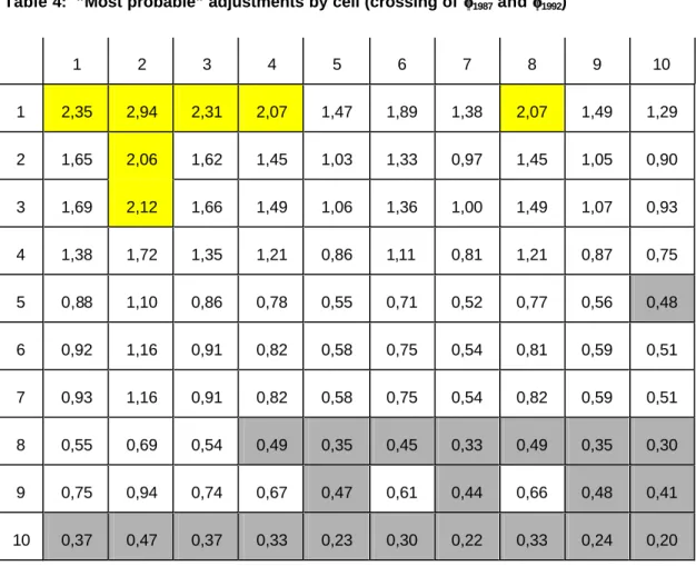
Given these preliminaries, we solve the Schrödinger system (7) by the method of iterative proportional fitting. This gives the "most probable" adjusted two-dimensional density matrix G reported in table 3 and the corresponding Schrödinger multipliers plotted in figure 2. Table 4 reports all cross-products of the Schrödinger multipliers, i.e. the matrix of adjustment coefficients (φi,1987×φj,1992)i,j = 1,...,10. These numbers show by how much one must multiply a cell of men's density matrix to get the "most probable" adjusted density. A closer examination of this matrix reveals that large values (values greater than 2) are concentrated in the north-west corner of the matrix whereas small values (values lower than 0.5) are concentrated in the south-east corner of the matrix.¹² This means, for example, that the probability of being in the lowest income class in 1987 and in the second income class in 1992 is nearly three times as large for women compared to men, according to the "most probable" adjustment. Similarly, the probability of being in both years in the highest income class is five times lower for women compared to men. Generally speaking, one must increase the probabilities to be in the low income classes and reduce those for being in the high income classes.

The plots of the Schrödinger multipliers in figure 2 show that the downward adjustments are due to the distribution in 1987 (φi,1987 < 1 for i ≥ 4) whereas the upward adjustments are primarily due to the distribution in 1992 (φi,1992 > 1 for i ≤ 4 and (φi,1992 ≈ 1 for i ≥ 5). This makes sense given the observed shift in the distribution documented in figure 1.

As mentioned in the theoretical part, we can use the relative entropy of the "most probable"

adjusted density matrix (matrix in table 3) with respect to men's density matrix (matrix in table 1) to test whether the adjustments are statistically significant. The value of relative entropy is 0.2069 and the value of the corresponding test statistic (9) is 386.89. Given that the critical value is 28.87 for the 5 percent significance level, we must clearly reject our hypothesis.¹³

Often it is more convenient to interpret the transition matrices instead of the two-dimensional densities. We have therefore computed the ”most probable” adjusted transition as indicated in equation (8). The result is reported in table 5. It shows only two significant changes at the 5

12 This pattern is typical. If we repeat this exercise for other time periods, we obtain nearly the same results.

13 The relative entropy of the ”true” density matrix estimated from the data is 0.2839 and therefore even larger.

Thus the ”true” density matrix is even further away from our hypothesis.

(19)

percent level: cells (2,2) and (3,2). In both cases the probabilities are adjusted upwards meaning that women have a significantly higher propensity to stay in the second income class and to fall back from the third income class to the second. Given the great similarity between the transition matrices which is also reflected in similar mobility indices, we conclude that the differences between the two-dimensional density matrices are largely due to the differences in the initial income distribution inherited from the past than to the income dynamics per se.

5. Conclusion

This paper has proposed a new approach to evaluate theories on the dynamics of income distributions. We hope to have demonstrated the validity and the usefulness of our method. Of course, further applications are necessary to arrive at a final judgment. The example of this paper was just a first test. The PSID data provided more information than we actually needed.

We could have, in principle, estimated the transition matrix for women from the data and compared it to the transition matrix of men using conventional statistical methods. The advantage of using the PSID data was that it allowed us to check whether our adjustments went into the ”right” direction, as they actually did.

In the future we hope to apply our method to issues where such additional information is not available. We could for example investigate the differences in the dynamics of income distributions across economies or across time. Or we could use our approach to evaluate specific theories of income dynamics as proposed by Conlisk (1990), Dardanoni (1994) or Wagner (1978).

The approach should also provide new insights in the ”empirics of economic growth” which studies the evolution of the cross-country income distribution (Quah 1996; Durlauf and Quah 1998). This literature has not yet gone beyond the simple estimation of transition matrices.

On the methodological side it would perhaps be desirable to extend our analysis to continuous random variables. This would circumvent the problem of choosing a somewhat arbitrary partition of the state space. Although it is not possible to carry over the combinatoric argument to the continuous state space case, the relative entropy is still well defined. Thus it is possible to extend the analysis from discrete to continuous state spaces by replacing the Schrödinger equation system (7) by a corresponding functional equation system. The extension to continuous time Markov processes, however, goes far beyond the scope of this paper (Föllmer 1988; Aebi and Nagasawa 1992).

(20)

References

Aebi, R. (1996): Schrödinger’s Time-Reversal of Natural Laws. The Mathematical Intelligencer 18: 62–67.

Aebi, R., and M. Nagasawa (1992): Large Deviations and the Propagation of Chaos for Schrödinger Processes. Probability Theory and Related Fields 94: 53–68.

Aebi, R. (1997): Contingency Tables with Prescribed Marginals. Statistical Papers 38: 219–29.

Atkinson, A. B. (1997): Bringing Income Distribution in from the Cold. Economic Journal 107:

297–321.

Barro, R. J., and X. Sala-i-Martin (1992): Convergence. Journal of Political Economy 100: 223–

51.

Billingsley, P. (1961): Statistical Inference for Markov Processes. Chicago: University of Chicago Press.

Champernowne, D. G. (1953): A Model of Income Distribution. Economic Journal 63: 318–51.

Conlisk, J. (1990): Monotone Mobility Matrices. Journal of Mathematical Sociology 15: 173–91.

Dardanoni, V. (1994): Income Distribution Dynamics: Monotone Markov Chains Make Light Work. Discussion Paper 94–16. University of California, San Diego.

Deming, W. E. and F. F. Stephan (1940): On a Least Squares Adjustment of a Sampled Frequency Table when the Expected Marginal Totals are Known. Annals of Mathematical Statistics 11: 427–44.

Durlauf, S. N., and D. T. Quah (1998): The New Empirics of Economic Growth. In Handbook of Macroeconomics, eds. J. B. Taylor and M. Woodford. Forthcoming.

Ellis, R. S. (1985): Entropy, Large Deviations, and Statistical Mechanics. New York: Springer- Verlag.

Föllmer, H. (1988): Random Fields and Diffusion Processes. École d´Été de Saint Flour XV - XVII. Lecture Notes in Mathematics 1362. New York: Springer-Verlag.

Gottschalk, P. (1997): Inequality, Income Growth, and Mobility: The Basic Facts. Journal of Economic Perspectives 11: 21–40.

(21)

Haberman, S. J. (1984): Adjustment by Minimum Discriminant Information. Annals of Statistics 12: 971–88.

Hillman, C. (1996): An Entropy Primer. Mimeo retrieved from URL:

<http://www.math.washington.edu/~hillman>

Ireland, C. T. and S. Kullback (1968): Contingency Tables with given Marginals. Biometrika 55:

179–88.

Kullback, S. (1959): Information Theory and Statistics. New York: John Wiley.

Quah, D. T. (1996): Convergence Empirics Across Economies with (Some) Capital Mobility.

Journal of Economic Growth 1: 95–124.

Schluter, C. (1998): Statistical Inference with Mobility Indices. Economics Letters 59: 157–62.

Shorrocks, A. F. (1978): The Measurement of Mobility. Econometrica 46: 1013–24.

Smith, J. H. (1947): Estimation of Linear Functions of Cell Proportions. Annals of Mathematical Statistics 13: 166–78.

Trede, M. (1998): Statistical Inference in Mobility Measurement: Sex Differences in Earnings Mobility. Jahrbücher für Nationalökonomie und Statistik forthcoming.

Wagner, M. (1978): On Comparisons of Distribution Processes. In Personal Income Distribution, eds. W. Krelle and A. F. Shorrocks. Amsterdam: North-Holland, 141–58.

(22)

Table 1: Two-dimensional density of men’s income in 1987 and 1992

(23)

Table 2: Men’s income transition matrix between 1987 and 1992

Shorrocks mobility index and its standard deviation: 0.80226 (0.01378)

(24)

Table 3: "Most probably" adjusted two-dimensional density matrix

Shading indicates a value significantly different at the 5 percent level from those of men’s density matrix in table 1

values above the 95%-confidence-interval for the two-dimensional density of men

values below the 95%-confidence-interval for the two-dimensional density of men

(25)

Table 4: ”Most probable” adjustments by cell (crossing of φφ1987 and φφ1992)

1 2 3 4 5 6 7 8 9 10

1 2,35 2,94 2,31 2,07 1,47 1,89 1,38 2,07 1,49 1,29 2 1,65 2,06 1,62 1,45 1,03 1,33 0,97 1,45 1,05 0,90 3 1,69 2,12 1,66 1,49 1,06 1,36 1,00 1,49 1,07 0,93 4 1,38 1,72 1,35 1,21 0,86 1,11 0,81 1,21 0,87 0,75 5 0,88 1,10 0,86 0,78 0,55 0,71 0,52 0,77 0,56 0,48 6 0,92 1,16 0,91 0,82 0,58 0,75 0,54 0,81 0,59 0,51 7 0,93 1,16 0,91 0,82 0,58 0,75 0,54 0,82 0,59 0,51 8 0,55 0,69 0,54 0,49 0,35 0,45 0,33 0,49 0,35 0,30 9 0,75 0,94 0,74 0,67 0,47 0,61 0,44 0,66 0,48 0,41 10 0,37 0,47 0,37 0,33 0,23 0,30 0,22 0,33 0,24 0,20

values higher than 2.0

values lower than 0.5

(26)

Table 5: ”Most probably” adjusted transition matrix

Shorrocks mobility index and its standard deviation: 0.80684 (0.01988)

Shading indicates a value significantly different at the 5 percent level from those of men’s transition matrix in table 2. Both values lie above the 95%-confidence-interval for the transition matrix of men.

(27)

Figure 1

(28)

Figure 2: ”Most probable” adjustments

Evaluating Theories of the Income Dynamics: A Probabilistic Approach

IHS Economics Series Working Paper 61