Automated Detection of Non-Termination and NullPointerExceptions for Java Bytecode
?Marc Brockschmidt, Thomas Str¨oder, Carsten Otto, and J¨urgen Giesl
LuFG Informatik 2, RWTH Aachen University, Germany
Abstract. Recently, we developed an approach for automated termina- tion proofs of Java Bytecode(JBC), which is based on constructing and analyzing termination graphs. These graphs represent all possible pro- gram executions in a finite way. In this paper, we show that this approach can also be used to detectnon-termination orNullPointerExceptions.
Our approach automatically generateswitnesses, i.e., calling the program with these witness arguments indeed leads to non-termination resp. to aNullPointerException. Thus, we never obtain “false positives”. We implemented our results in the termination proverAProVEand provide experimental evidence for the power of our approach.
1 Introduction
To use program verification in the software development process, one is not only interested in proving the validity of desired program properties, but also in providing a witness (i.e., a counterexample) if the property is violated.
Our approach is based on our earlier work to prove termination of JBC[4, 6, 17]. Here, aJBCprogram is first automatically transformed to atermination graph by symbolic evaluation. Afterwards, a term rewrite system is generated from the termination graph and existing techniques from term rewriting are used to prove termination of the rewrite system. As shown in the annualInternational Termination Competition,1 our corresponding tool AProVEis currently among the most powerful ones for automated termination proofs of Javaprograms.
Termination graphsfinitely represent all runs through a program for a certain set of input values. Similar graphs were used for many kinds of program analysis (e.g., to improve the efficiency of software verification [7], or to ensure termi- nation of program optimization [22]). In this paper, we show that termination graphs can also be used to detect non-termination andNullPointerExceptions.
In Sect. 2, we recapitulate termination graphs. In contrast to [4, 6, 17], we also handle programs witharrays and we present an algorithm tomerge abstract states in a termination graph which is needed in order to keep termination graphs finite. In Sect. 3 we show how to automatically generatewitness states (i.e., suit- able inputs to the program) which result in errors likeNullPointerExceptions.
Sect. 4 presents our approach to detect non-termination. Here, we use an SMT
?Supported by the DFG grant GI 274/5-3, the G.I.F. grant 966-116.6, and the DFG Research Training Group 1298 (AlgoSyn).
1 Seehttp://www.termination-portal.org/wiki/Termination_Competition
solver to find different forms of non-terminating loops and the technique of Sect. 3 is applied to generate appropriate witness states.
Concerning the detection of NullPointerExceptions, most existing tech- niques try to prove absence of such exceptions (e.g., [15, 23]), whereas our ap- proach tries to prove existence ofNullPointerExceptions and provides coun- terexamples which indeed lead to such exceptions. So in contrast to bug finding techniques like [2, 9], our approach does not yield “false positives”.
Methods to detect non-termination automatically have for example been studied for term rewriting (e.g., [11, 19]) and logic programming (e.g., [18]). We are only aware of two existing tools for automated non-termination analysis of Java: The tool Julia transforms JBC programs into constraint logic programs, which are then analyzed for non-termination [20]. The toolInvel[24] investigates non-termination of Java programs based on a combination of theorem proving and invariant generation using the KeY [3] system. In contrast to Julia and to our approach, Invelonly has limited support for programs operating on the heap. Moreover, neitherJulianorInvelreturn witnesses for non-termination. In Sect. 5 we compare the implementation of our approach in the toolAProVEwith Julia and Invel and show that our approach indeed leads to the most powerful automated non-termination analyzer for Javaso far.
Moreover, [14] presents a method for non-termination proofs of Cprograms.
In contrast to our approach, [14] can deal with non-terminating recursion and in- teger overflows. On the other hand, [14] cannot detectnon-periodicnon-termina- tion (where there is no fixed sequence of program positions that is repeated in- finitely many times), whereas this is no problem for our approach, cf. Sect. 4.2.
There also exist tools for testingCprograms in a randomized way, which can detect candidates for potential non-termination bugs (e.g., [13, 21]). However, they do not provide a proof for non-termination and may return “false positives”.
2 Termination Graphs
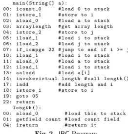
p u b l i c c l a s s L o o p {
p u b l i c s t a t i c v o i d m a i n ( S t r i n g [] a ){
int i = 0;
int j = a . l e n g t h ; w h i l e ( i < j ) {
i += a [ i ]. l e n g t h (); }}}
Fig. 1.JavaProgram
m a i n ( S t r i n g [] a ):
00: i c o n s t _ 0 # l o a d 0 to s t a c k 01: i s t o r e _ 1 # s t o r e to i 02: a l o a d _ 0 # l o a d a to s t a c k 03: a r r a y l e n g t h # get a r r a y l e n g t h 04: i s t o r e _ 2 # s t o r e to j 05: i l o a d _ 1 # l o a d i to s t a c k 06: i l o a d _ 2 # l o a d j to s t a c k 07: i f _ i c m p g e 22 # j u m p to end if i >= j 10: i l o a d _ 1 # l o a d i to s t a c k 11: a l o a d _ 0 # l o a d a to s t a c k 12: i l o a d _ 1 # l o a d i to s t a c k 13: a a l o a d # l o a d a [ i ]
14: i n v o k e v i r t u a l l e n g t h # c a l l l e n g t h () 17: i a d d # add l e n g t h and i 18: i s t o r e _ 1 # s t o r e to i 19: g o t o 05
22: r e t u r n l e n g t h ():
00: a l o a d _ 0 # l o a d t h i s to s t a c k 01: g e t f i e l d c o u n t # l o a d c o u n t f i e l d 04: i r e t u r n # r e t u r n it
Fig. 2.JBCProgram We illustrate our approach by the
main method of the Java program in Fig. 1. The main method is the en- try point when starting a program. Its only argument is an array of String objects corresponding to the argu- ments specified on the command line.
To avoid dealing with all syntactic constructs of Java, we analyze JBC instead. JBC [16] is an assembly-like
object-oriented language designed as intermediate format for the execution of Java. The corresponding JBCfor our example, obtained automatically by the standard javaccompiler, is shown in Fig. 2 and will be explained in Sect. 2.2.
The methodmainincrementsiby the length of thei-th input string untili exceeds the numberjof input arguments. It combines two typical problems:
(a) The accesses toa.lengthanda[i].length()are not guarded by appropri- ate checks to ensure memory safety. Thus, ifaora[i]arenull, the method ends with a NullPointerException. While this cannot happen when the method is used as an entry point for the program, another method could for instance containString[] b = {null}; Loop.main(b).
(b) The method may not terminate, as the input arguments could contain the empty string. If a[i] = "", then the counter i is not increased, leading tolooping non-termination, as the same program state is visited again and again. For instance, the calljava Loop ""does not terminate.
We show how to automatically detect such problems and to synthesize appropri- ate witnesses in Sect. 3 and 4. Our approach is based ontermination graphsthat over-approximate all program executions. After introducing our notion of states in Sect. 2.1, we describe the construction of termination graphs in Sect. 2.2.
Sect. 2.3 shows how to create “merged” states representing two given states.
2.1 Abstract States
Our approach is related toabstract interpretation [8], since the states in termi- nation graphs areabstract, i.e., they represent a (possibly infinite) set of concrete system configurations of the program. We define the set of all states asStates= (PPos×LocVar×OpStack)∗×({⊥} ∪Refs)×Heap×Annotations.
Consider the program from Fig. 1. The initial stateAin Fig. 3 represents all system configurations entering themainmethod with arbitrary tree-shaped (and thus, acyclic) non-nullarguments. A state consists of four parts: the call stack, exception information, the heap, and annotations for possible sharing effects.
00|a:a1|ε
a1:String[ ]i1 i1: [≥0]
Fig. 3.StateA
The call stack consists of stack frames, where several frames may occur due to method calls. For readability, we exclude recursive programs, but our results easily extend to the approach of [6] for recursion. We also disregard multi- threading, reflection, static fields, static initialization of classes, and floats.
Each stack frame has three components. We write the frames of the call stack below each other and separate their components by “|”. The first component of a frame is the program position, indicated by the number of the next instruction (00in Fig. 3). The second component represents the local variables by a list of references to the heap, i.e., LocVar=Refs∗. To avoid a special treatment of primitive values, we also represent them by references. In examples, we write the names of variables instead of their indices. Thus, “a:a1” means that the value of the 0-th local variableais the referencea1(i.e.,a1is the address of an array ob- ject). Of course, different local variables can point to the same address. The third component is the operand stack thatJBCinstructions work on, whereOpStack
=Refs∗. The empty stack is “ε” and “i6, i4” is a stack withi6 on top.
Information about thrown exceptions is represented in the second part of our states. If no exception is currently thrown, this part is ⊥(which we do not display in example states). Otherwise it is a reference to the exception object.
Below the call stack, information about the heap is given by a partial func- tion fromHeap=Refs →(Integers ∪ Unknown ∪ Instances ∪ Arrays
∪ {null}) and by a set of annotations which specify possible sharing effects.
Our representation of integers abstracts from the different bounded types of integers in Java and considers arbitrary integer numbers instead (i.e., we do not handle overflows). To represent unknown integer values, we use possibly unbounded intervals, i.e.,Integers={{x∈Z|a≤x≤b} |a∈Z∪{−∞}, b∈ Z∪ {∞}, a≤b}. We abbreviate (−∞,∞) byZand intervals like [0,∞) by [≥0].
So “i1: [≥0]” means that any non-negative integer can be at the addressi1. Classnamescontains the names of all classes and interfaces in the program.
Types = Classnames∪ {t[ ] |t ∈Types} contains Classnames and all re- sulting array types. So a type t[ ] can be generated from any typetto describe arrays with entries of typet.2 We call t0 asubtype oft ifft0 =t; ort0 extends3 orimplements a subtype of t; ort0= ˆt0[ ],t= ˆt[ ], and ˆt0 is a subtype of ˆt.
The values in Unknown = Types×{?} represent tree-shaped (and thus acyclic) objects and arrays where we have no information except the type. For example, for a classListwith the fieldnextof typeList, “o1:List(?)” means that the object at addresso1 isnullor of a subtype ofList.
Instancesrepresent objects of some class. They are described by the values of their fields, i.e.,Instances=Classnames×(FieldIDs→Refs). For cases where field names are overloaded, theFieldIDsalso contain the respective class name to avoid ambiguities, but we usually do not display it in our examples. So
“o1:List(next=o2)” means that at the addresso1, there is aListobject and the value of its field next is o2. For all (cl, f)∈ Instances, the function f is defined for all fields of the classcl and all of its superclasses.
In contrast to our earlier papers [4, 6, 17], in this paper we also show how to handlearrays. An array can be represented by an element fromTypes×Refs denoting the array’s type and length (specified by a reference to an integer value).
For instance, “a1:String[ ]i1” means that at the addressa1, there is aString array of length i1. Alternatively, the array representation can also contain an additional list of references for the array entries. So “a2:String[ ]i1 {o1, o2}”
denotes that at the address a2, we have a String array of length i1, and its entries are o1 and o2 (displayed in the Java syntax “{. . .}” for arrays). Thus, Arrays= (Types×Refs) ∪ (Types×Refs×Refs∗).
In our representation, no sharing can occur unless explicitly stated. So an abstract state containing the references o1, o2 and not mentioning that they could be sharing, only represents concrete states where o1 and the references reachable from o1 are disjoint4 from o2 and the references reachable from o2.
2 We do not consider arrays of primitives in this paper, but our approach can easily be extended to handle them, as we did in our implementation.
3 For example, any type (implicitly)extends the typejava.lang.Object.
4 Disjointness is not required for references pointing toIntegersor tonull.
Moreover, then the objects ato1ando2must be tree-shaped (and thus acyclic).
Certain sharing effects are represented directly (e.g., “o1:List(next=o1)” is a cyclic singleton list). Other sharing effects are represented by three kinds ofan- notations, which are only built for referencesowhereh(o)∈/ Integers∪ {null}
for the heaph. The first kind of annotation is calledequality annotation and has the form “o1 =? o2”. Its meaning is that the addresses o1 and o2 could be equal. We only use such annotations if the value of at least one of o1 and o2
is Unknown. Joinability annotations are the second kind of annotation. They express that two objects “may join” (o1 %$o2). We say that a non-integer and non-nullreferenceo0 is a direct successor ofoin a states(denotedo→so0) iff the object at addresso has a field whose value iso0 or if the array at address o haso0 as one of its entries. The meaning of “o1%$o2” is that there could be an o witho1→∗s o ←+s o2 or o1 →+s o←∗s o2, i.e.,o is a common successor of the two references. However, o1%$o2does not implyo1=?o2. Finally, as the third type of annotations, we usecyclicity annotations “o!” to denote that the object at addressois not necessarily tree-shaped (so in particular, it could be cyclic).
2.2 Constructing Termination Graphs
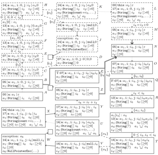
Starting from the initial stateA, the termination graph in Fig. 4 is constructed by symbolic evaluation. In the first step, we have to evaluateiconst 0, i.e., we load the integer 0 on top of the operand stack. The second instructionistore 1 stores the value 0 on top of the operand stack in the first local variablei.5
After that, the value of the 0-th local variable a (the array in the input argument) is loaded on the operand stack and the instruction arraylength retrieves its (unknown) lengthi1. That value is then stored in the second local variablejusing the instructionistore 2. This results in the stateB in Fig. 4.
We connectAandB by a dotted arrow, indicating several evaluation steps (i.e., we omitted the states betweenAandB for space reasons in Fig. 4).
From B on, we load the values of iand j on the operand stack and reach C.6 The instruction if icmpge branches depending on the relation of the two elements on top of the stack. However, based on the knowledge inC, we cannot determine whetheri >= jholds. Thus, we perform a case analysis (calledinteger refinement [4, Def. 1]), obtaining two new statesD andE. We label therefine- ment edges fromCtoDandE(represented by dashed arrows) by the reference i1that was refined. InD, we assume thati >= jholds. Hence,i1(corresponding to j) is ≤ 0 and from i1 : [≥0] in state C we conclude that i1 is 0. We thus reach instruction22(return), where the program ends (denoted by).
InE, we consider the other case and replacei1 byi2, which only represents positive integers. We mark what relation holds in this case by labeling the eval- uation edge from E to its successor with 0 < i2. In general, we always use a
5 If we have a reference whose value is from a singleton interval like [0,0] or null, we replace all its occurrences in states by 0 resp. bynull. So in stateB, we simply write “i: 0”. Such abbreviations will also be used in the labels of edges.
6 The box around C and the following states is dashed to indicate that these states will be removed from the termination graph later on.
00|a:a1|ε
a1:String[ ]i1 i1: [≥0]
A 05|a:a1,i: 0,j:i1|ε a1:String[ ]i1 i1: [≥0]
B 07|a:a1,i: 0,j:i1|i1,0 a1:String[ ]i1 i1: [≥0] C
07|a:a1,i: 0,j: 0|0,0 a1:String[ ] 0 07|a:a1,i: 0,j:i2|i2,0 D
a1:String[ ]i2 i2: [>0]
E 13|a:a1,i: 0,j:i2|0,a1,0 a1:String[ ]i2 i2: [>0]
F a1[0] :o1
13|a:a1,i: 0,j:i2|0,a1,0 a1:String[ ]i2 i2: [>0]
o1:String(?) a1%$o1
G 14|a:a1,i: 0,j:i2|o1,0 a1:String[ ]i2 i2: [>0]
o1:String(?) a1%$o1
H 14|a:a1,i: 0,j:i2|o2,0 a1:String[ ]i2 i2: [>0]
o2:String(count=i3, . . .) i3: [≥0] a1%$o2
K
14|a:a1,i: 0,j:i2|null,0 a1:String[ ]i2 i2: [>0]
I
exception:o3
14|a:a1,i: 0,j:i2|null,0 a1:String[ ]i2 i2: [>0]
o3:NullPointerExc(. . .) J
00|this:o2|ε 17|a:a1,i: 0,j:i2|0 a1:String[ ]i2 i2: [>0]
o2:String(count=i3, . . .) i3: [≥0] a1%$o2
L
05|a:a1,i:i4,j:i2|ε a1:String[ ]i2 i2: [>0]
i4: [≥0]
M
05|a:a1,i:i4,j:i6|ε a1:String[ ]i6 i6: [≥0]
i4: [≥0]
N
07|a:a1,i:i4,j:i6|i6,i4
a1:String[ ]i6 i6: [≥0]
i4: [≥0]
O
T:07|a:a1,i:i4,j:i6|i6,i4 a1:String[ ]i6 i6: [≥0]
i4: [≥0]
P
F:07|a:a1,i:i4,j:i6|i6,i4 a1:String[ ]i6 i6: [≥0]
i4: [≥0]
Q
13|a:a1,i:i4,j:i6|i4,a1,i4 a1:String[ ]i6 i6: [≥0]
i4: [≥0]
R
a1[i4] :o4
13|a:a1,i:i4,j:i6|i4,a1,i4 a1:String[ ]i6 i6: [≥0]
o4:String(?) a1%$o4 i4: [≥0]
S
14|a:a1,i:i4,j:i6|o4,i4
a1:String[ ]i6 i6: [≥0]
o4:String(?) a1%$o4
i4: [≥0]
14|a:a1,i:i4,j:i6|null,i4 T a1:String[ ]i6 i6: [≥0]
i4: [≥0]
V exception:o6
14|a:a1,i:i4,j:i6|null,i4 a1:String[ ]i6 i6: [≥0]
i4: [≥0]
o6:NullPointerExc(. . .) W
14|a:a1,i:i4,j:i6|o5,i4 a1:String[ ]i6 i6: [≥0]
o5:String(count=i7, . . .) i4: [≥0]i7: [≥0] a1%$o5
U 04|this:o5|i7
17|a:a1,i:i4,j:i6|i4
a1:String[ ]i6 i6: [≥0]
o5:String(count=i7, . . .) i4: [≥0]i7: [≥0] a1%$o5
X
17|a:a1,i:i4,j:i6|i7, i4 a1:String[ ]i6 i6: [≥0]
i4: [≥0] i7: [≥0]
Y 05|a:a1,i:i8,j:i6|ε a1:String[ ]i6 i6: [≥0]
i8: [≥0]
Z {i1}
{i1} 0< i2
{a1,0}
0≤0,0< i2
{o1}
{o1}
i4=i3+0
{i4, i6} {i4, i6}
i4< i6
{a1, i4}
0≤i4, i4< i6
{o4} {o4} i8=i7+i4
Fig. 4.Termination Graph
fresh reference name likei2 when generating new values by a case analysis, to ensure single static assignments, which will be useful in the analysis later on. We continue with instruction 10and load the values ofi,a, andion the operand stack, obtaining stateF. To evaluateaaload(i.e., to load the 0-th element from the array a1 on the operand stack), we add more information about a1 at the index 0 and label the refinement edge fromF toGaccordingly. InG, we created some objecto1for the 0-th entry of the arraya1and marked thato1is reachable froma1 by adding the joinability annotationa1%$o1.7
Now evaluation ofaaloadmoveso1 to the operand stack in stateH. When- ever an array access succeeds, we label the corresponding edge by the condition that the used index is≥0 and smaller than the length of the array.
InH, we need toinvokethe methodlength()on the objecto1. However, we do not know whethero1isnull(which would lead to aNullPointerException).
7 If we had already retrieved another valueo0 from the array a1, it would also have been annotated witha1%$o0and we would consequently addo1%$o0 ando1=?o0 when retrievingo1, indicating that the two values may share or even be equal.
Hence, we perform aninstance refinement [4, Def. 5] and label the edges from H to the new states I and K by the reference o1 that is refined. In I, o1 has the valuenull. In K, we replace the referenceo1 byo2, pointing to a concrete String object with unknown field values. In Fig. 4, we only display the field count, containing the integer reference i3. In this instance refinement, one uses the special semantics of the pre-definedStringclass to conclude thati3can only point to a non-negative integer, ascountcorresponds to thelengthof the string.
In I, further evaluation results in a NullPointerException. A corresponding exception object o3 is generated and the exception is represented in J. As no exception handler is defined, evaluation ends and the program terminates.
InK, callinglength()succeeds. InL, a new stack frame is put on top of the call stack, where the implicit argumentthis is set too2. In the called method length(), we loado2on the operand stack and get the valuei3of its fieldcount.
We then return fromlength(), add the returned valuei3to 0, and store the re- sult in the variablei. Afterwards, we jump back to instruction05. This is shown in stateM and the computationi4=i3+ 0 is noted on the evaluation edge.
But nowM is at the same program position asB. Continuing our symbolic evaluation would lead to an infinite tree, as we would always have to consider the case where the loop conditioni < jis still true. Instead, our goal is to obtain a finite termination graph. The solution is to automatically generate a new stateN which represents all concrete states that are represented by B orM (i.e.,N re- sults frommerging BandM). Then we can insertinstance edges fromB andM toN (displayed by double arrows) and continue the graph construction withN.
2.3 Instantiating and Merging States
To find differences between states and to merge states, we introduce state po- sitions. Such a position describes a “path” through a state, starting with some local variable, operand stack entry, or the exception object and then continu- ing through fields of objects or entries of arrays. For the latter, we use the set ArrayIdxs={[j]|j≥0} to describe the set of all possible array indices.
Definition 1 (State Positions SPos).Lets= (hfr0, . . . ,frni, e, h, a)be a state where each stack frame fri has the form (ppi, lvi, osi). Then SPos(s) is the smallest set containing all the following sequencesπ:
• π=lvi,j where 0≤i≤n,lvi=hoi,0, . . . , oi,mii,0≤j≤mi. Thens|π isoi,j.
• π=osi,j where0≤i≤n,osi=ho0i,0, . . . , o0i,k
ii,0≤j≤ki. Thens|π iso0i,j.
• π=excife6=⊥. Thens|π ise.
• π=π0v for some v ∈FieldIDs and some π0 ∈SPos(s) where h(s|π0) = (cl, f)∈Instances and wheref(v)is defined. Thens|π isf(v).
• π = π0 len for some π0 ∈ SPos(s) where h(s|π0) = (t, i) ∈ Arrays or h(s|π0) = (t, i, d)∈Arrays. Thens|π isi.
• π = π0[j] for some [j] ∈ ArrayIdxs and some π0 ∈ SPos(s), where h(s|π0) = (t, i,hr0, . . . , rqi)∈Arrays and0≤j ≤q. Thens|π isrj. For any positionπ, letπsdenote the maximal prefix ofπsuch thatπs∈SPos(s).
We writeπ if sis clear from the context.
For example, in stateK, the positionπ=os0,0 countrefers to the reference i3, i.e., we haveK|π =i3 and for the positionτ =lv0,0 len, we have K|τ =i2. As the fieldcountwas introduced betweenH andK by an instance refinement, we haveπ6∈SPos(H) and πH =os0,0, whereH|π =o1. We can now see that B andM only differ in the positions lv0,0 len,lv0,1, andlv0,2.
A states0is aninstanceof another states(denoteds0vs) if both are at the same program position and if whenever there is a references0|π, then either the values represented bys0|πin the heap ofs0 are a subset of the values represented bys|πin the heap ofsor else,π /∈SPos(s). Moreover, shared parts of the heap in s0 must also be shared ins. As we only consider verified JBCprograms, the fact that sands0 are at the same program position implies that they have the same number of local variables and their operand stacks have the same size. For a formal definition of “instance”, we refer to Def. 9 in the appendix, where we extended the “instance” definition from [4, Def. 3] to arrays.
For example,Bis not an instance ofM sincehB(B|lv0,2) = [0,∞)6⊆[1,∞) = hM(M|lv0,2) for the heapshB andhM of B and M. Similarly,M 6vB because hM(M|lv0,1) = [0,∞) 6⊆ {0} = hB(B|lv0,1). However, we can automatically synthesize a “merged” (or “widened”) state N with B v N and M v N by choosing the values for common positions π in B and M to be the union of the values in B and M, i.e., hN(N|π) = hB(B|π)∪hM(M|π). Thus, we have hN(N|lv0,2) = [0,∞)∪[1,∞) = [0,∞) andhN(N|lv0,1) ={0} ∪[0,∞) = [0,∞).
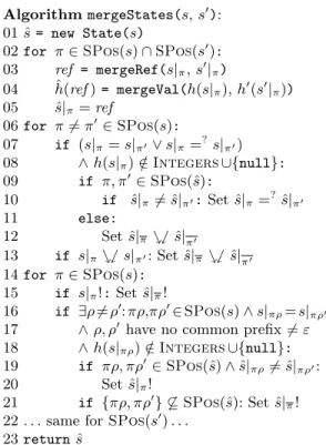
AlgorithmmergeStates(s,s0):
ˆ
s= new State(s)
for π∈SPos(s)∩SPos(s0):
ref = mergeRef(s|π,s0|π)
h(refˆ )= mergeVal(h(s|π),h0(s0|π)) s|ˆπ=ref
for π6=π0∈SPos(s):
if (s|π=s|π0∨s|π=?s|π0)
∧h(s|π)∈/Integers∪{null}:
if π, π0∈SPos(ˆs):
if ˆs|π6= ˆs|π0:Set ˆs|π=?s|ˆπ0
else:
Set ˆs|π%$s|ˆπ0
if s|π%$s|π0: Set ˆs|π%$s|ˆπ0
for π∈SPos(s):
if s|π!:Set ˆs|π!
if ∃ρ6=ρ0:πρ,πρ0∈SPos(s)∧s|πρ=s|πρ0
∧ρ, ρ0have no common prefix6=ε
∧h(s|πρ)∈/Integers∪{null}:
if πρ, πρ0∈SPos(ˆs)∧s|ˆπρ6= ˆs|πρ0: Set ˆs|π!
if {πρ, πρ0} 6⊆SPos(ˆs): Set ˆs|π! . . .same forSPos(s0). . .
returnsˆ
Fig. 5.Merging Algorithm
This merging algorithm is illus- trated in Fig. 5. Here,h, h0,ˆhrefer to the heaps of the statess, s0,s, respec-ˆ tively. With new State(s), we cre- ate a fresh state at the same program position as s. The auxiliary func- tion mergeRef is an injective map- ping from a pair of references to a fresh reference name. The func- tion mergeVal maps two heap val- ues to the most precise value from our abstract domains that represents both input values. For example, mergeVal([0,1],[10,15]) is [0,15], covering both input values, but also adding [2,9] to the set of represented values. For values of the same type, e.g.,String(count=i1, . . .) and String(count=i2, . . .), mergeVal re- turns a new object of same type with field values obtained by mergeRef, e.g., String(count=i3, . . .) where i3
= mergeRef(i1, i2). When merging values of differing types or null, a
value fromUnknownwith the most precise common supertype is returned.
To handle sharing effects, in a second step, we check if there are “sharing”
references at some positions π and π0 in s or s0 that do not share anymore in the merged state ˆs. Then we add the corresponding annotations to the maximal prefixes ˆs|π and ˆs|π0. Furthermore, we check if there are non-tree shaped objects at some position π in s or s0, i.e., if one can reach the same successor using different paths starting in positionπ. Then we add the annotation ˆs|π!.
Theorem 2. Lets, s0∈Statesandsˆ=mergeStates(s,s0). Thensvsˆws0.8 In our example, we used the algorithm mergeStates to create the stateN and draw instance edges fromB andM toN. Since the computation inN also represents the statesCtoM (marked by dashed borders), we now remove them.
We continue symbolic evaluation inN, reaching stateO, which is likeC. InC, we refined our information to decide whether the conditioni >= jofif icmpge holds. However, now this case analysis cannot be expressed by simply refining the intervals fromIntegers that correspond to the referencesi6 andi4(i.e., a relation likei4≥i6is not expressible in our states). Instead, we again generate successors for both possible values of the condition i >= j, but do not change the actual information about our values. In the resulting states P and Q, we mark the truth value of the conditioni >= jby “T” and “F”. The refinement edges fromOtoP andQare marked by the referencesi4andi6that are refined.
P leads to a program end, while we continue the symbolic evaluation inQ. As before, we label the refinement edge fromQtoRbyi4< i6.
R andS are like F and G. The refinement edge fromR to S is labeled by a1 and i4 which were refined in order to evaluate aaload (note that since we only reach R if i4 < i6, the array access succeeds). As in H, we then perform an instance refinement to decide whether calling length() on the object o4
succeeds, leading to U and V. From V, we again reach a program end after a NullPointerException was thrown in W. FromU, we reach X by evaluating the call to length(). Between X to Y, we return from length(). After that, we add the two non-negative integersi7 andi4, creating a non-negative integer i8. The edge fromY toZ is labeled by the computationi8=i7+i4.
Z is again an instance of N. We can also use the algorithm mergeStates to determine whether one state is an instance of another: When merging s, s0 to obtain a new state ˆs, one adaptsmergeStates(s, s0)such that the algorithm terminates with failure whenever we widen a value ofsor add an annotation to ˆs that did not exist ins(e.g., when we add ˆs|π=?s|ˆπ0 and there is nos|π=?s|π0).
Then the algorithm terminates successfully iff s0 v sholds. After drawing the instance edge fromZtoN (yielding acyclein our graph), all leaves of the graph are program ends and thus the graph construction is finished.
We now define termination graphs formally. We extend our earlier definition from [4] slightly by labeling edges with information about the performed refine- ments and about the relations of integers. LetRelOp={i◦i0 |i, i0∈Refs,◦ ∈ {<,≤,=,6=,≥, >}} denote the set of relations between two integer references such asi4< i6andArithOp={i=i0 ./ i00|i, i0, i00∈Refs, ./∈ {+,−,∗, /,%}}
8 For all proofs, we refer to the appendix.
denote the set of arithmetic computations such asi8=i7+i4.
Termination graphs are constructed by repeatedly expanding those leaves that do not correspond to program ends. Whenever possible, we use symbolic evaluation SyEv−→. Here,SyEv−→ extends the usual evaluation relation forJBCsuch that it can also be applied toabstractstates representing several concrete states.
For a formal definition ofSyEv−→, we refer to [4, Def. 6]. In the termination graph, the correspondingevaluation edgescan be labeled by a setC⊆ ArithOp∪RelOp which corresponds to the arithmetic operations and (implicitly) checked relations in the evaluation. For example, when accessing the indexiof an arrayasucceeds, we have implicitly ensured 0≤iandi<a.lengthand this is noted in C.
If symbolic evaluation is not possible, we refine the information for some referencesRby case analysis and label the resultingrefinement edges withR.
To obtain afinite graph, we create a more general state bymergingwhenever a program position is visited a second time in our symbolic evaluation and add appropriate instance edges to the graph. However, we require all cycles of the termination graph to contain at least one evaluation edge. By using an appro- priate strategy for merging resp. widening states, we can automatically generate a finite termination graph for any program.
Definition 3 (Termination Graph). A graph(V, E)withV ⊆States,E⊆ V × ({Eval} ×2ArithOp∪RelOp)∪({Refine} ×2Refs)∪ {Ins}
×V is a termi- nation graph if every cycle contains at least one edge labeled with someEvalC
and one of the following holds for each s∈V:
• s has just one outgoing edge (s,EvalC, s0), s SyEv−→ s0, and C is the set of integer relations that are checked (resp. generated) in this step
• the outgoing edges of s are (s,RefineR, s1), . . . ,(s,RefineR, sn) and {s1, . . . , sn} is a refinement of son the referencesR⊆Refs
• shas just one outgoing edge(s,Ins, s0) andsvs0
• shas no outgoing edge ands= (ε, e, h, a)(i.e., s is a program end)
The soundness proofs for the transformation fromJBCto termination graphs can be found in [4]. There, we show that ifcis a concrete state withcvsfor some statesin the termination graph, then theJBCevaluation ofc is represented in the termination graph. We refer to [6, 17] for methods to use termination graphs for termination proofs. In Sect. 3 and 4 we show how to use termination graphs to detectNullPointerExceptions and non-termination.
3 Generating Witnesses for NullPointerExceptions
In our example, an uncaught NullPointerException is thrown in the “error state” W, leading to a program end. Such violations of memory safety can be immediately detected from the termination graph.9
To report such a possible violation of memory safety to the user, we now show
9 InC,memory safetymeans absence of (i) accesses tonull, (ii) dangling pointers, and (iii) memory leaks [25]. InJava, theJVMensures (ii) and (iii), and onlyNullPoin- terExceptions andArrayIndexOutOfBoundsExceptions can destroy memory safety.
how to automatically generate a witness (i.e., an assignment to the arguments of the program) that leads to the exception. Our termination graph allows us to generate such witnesses automatically. This technique for witness generation will also be used to construct witnesses for non-termination in Sect. 4.
So our goal is to find awitness state A0 for the initial stateAof the method main w.r.t. the “error state”W. This stateA0 describes a subset of arguments, all of which lead to an instance ofW, i.e., to aNullPointerException.
Definition 4 (Witness State).Lets, s0, w∈States. The states0is awitness state for sw.r.t.wiffs0vs ands0SyEv−→∗w0 for some statew0 vw.
To obtain a witness state A0 for A automatically, we start with the error state W and traverse the edges of the termination graph backwards until we reach A. In general, let s0, s1, . . . , sn =w be a path in the termination graph from the initial states0 to the error statesn. Assuming that we already have a witness states0i forsi w.r.t.w, we show how to generate a witness states0i−1for si−1 w.r.t. w. To this end, we revert the changes done to the state si−1 when creating the statesi during the construction of the termination graph (i.e., we apply the rules for termination graph construction “backwards”). Of course, this generation of witness states can fail (in particular, this happens for error states that are not reachable from any concrete instantiation of the initial states0). So in this way, our technique for witness generation is also used as a check whether certain errors can really result from initial method calls.
In our example, the error state isW. Trivially,W itself is a witness state for W w.r.t.W. The only edge leading toW is fromV. Thus, we now generate a witness stateV0forV w.r.t.W. The edge fromV toW represents the evaluation of the instruction invokevirtual that triggered the exception. Reversing this instruction is straightforward, as we only have to remove the exception object fromW again. Thus,V is a witness state forV w.r.t.W.
The only edge leading to V is a refinement edge from T. As a refinement corresponds to a case analysis, the information in the target state is more precise.
Hence, we can reuse the witness state forV, since V is an instance ofT. So V is also a witness state for T w.r.t.W. 13|a:a2,i: 0,j: 1|0,a2,0
a2:String[ ] 1{null}
Fig. 6.StateR0 To reverse the edge betweenT andS, we have to undo
the instructionaaload. This is easy since S contains the
information that the entry at indexi4in the arraya1iso4. Thus the witness state S0forSw.r.t.W is likeS, but hereo4’s value is not an unknown object, butnull.
Reversing the refinement betweenSandRis more complex. Note that not every state represented byRleads to aNullPointerException. InSwe had noted the relation between the newly created referenceo4and the original arraya1. In other words, inSwe know thata1[i4] iso4, whereo4has the valuenullin the witness stateS0forS. But inR,o4is missing. To solve this problem, in the witness state R0 for R, we instantiate the abstract arraya1 by a concrete one that contains the entrynullat the indexi4. We use a simple heuristic10to choose a suitable
10Such heuristics cannot affect soundness, but just the power of our approach (choosing unsuitable values may prevent us from finding a witness for the initial state).
lengthi6for this concrete array, which tries to find “minimal” values. Here, our heuristic chooses a1 to be an array of length one (i.e., i6 is chosen to be 1), which only contains the entry null (at the index 0, i.e., i4 is chosen to be 0).
The resulting witness state R0 forRw.r.t.W is displayed in Fig. 6.
0|a:a2|ε
a2:String[ ] 1{null}
Fig. 7.StateA0 Reversing the evaluation steps betweenRand Qyields
a witness stateQ0 forQw.r.t.W. FromO toQ, we have a refinement edge and thus,Q0 is also a witness forO.
The steps fromN toO can also be reversed easily. In N, we use a heuristic to decide whether to follow the incoming edge fromZ or fromB. Our heuristic chooses B as it is more concrete than Z. From there, we continue our reversed evaluation until we reach a witness stateA0for the initial stateAof the method w.r.t.W, cf. Fig. 7. So any instance ofA0 evaluates to an instance ofW, i.e., it leads to aNullPointerException. If themainmethod is called directly (as the entry point of the program), then theJVMensures that the input array does not containnullreferences. But if themainmethod is called from another method, then this violation of memory safety can indeed occur, cf. problem (a) in Sect. 2.
The following theorem summarizes our procedure to generate witness states.
If there is an edge from a states1to a states2 in the termination graph and we already have a witness states02fors2w.r.t.w, then Thm. 5 shows how to obtain a witness states01fors1w.r.t.w. Hence, by repeated application of this construc- tion, we finally obtain a witness state for the initial state of the method w.r.t.w.
If there is anevaluation edgefroms1tos2, then we first apply the reversed rules for symbolic evaluation on s02. Afterwards, we instantiate the freshly appearing references (for example, those overwritten by the forward symbolic evaluation) such thats01is indeed an instance ofs1. If there is arefinement edge froms1 to s2, then the witness states01 is like s02, but when reading from abstract arrays (such as betweenR and S), we instantiate the array to a concrete one ins01. If there is aninstance edge froms1tos2, then weintersect the statess1ands02 to obtain a representation of those states that are instances of boths1 ands02. Theorem 5 (Generating Witnesses). Let(s1, l, s2)be an edge in the termi- nation graph and lets02 be a witness state fors2 w.r.t.w. Lets01∈Stateswith:
• ifl=EvalC, thens01is obtained froms02by applying the symbolic evaluation used between s1 and s2 backwards. In s01, we instantiate freshly appearing variables such thats01vs1 ands01SyEv−→ s02 holds.
• ifl=RefineR, thens01vs02.
• ifl=Ins, thens01=s1∩s02 (for the definition of∩, see [6, Def. 2]).
Thens01 is a witness state fors1 w.r.t. w.
4 Proving Non-Termination
Now we show how to prove non-termination automatically. Sect. 4.1 introduces a method to detect looping non-termination, i.e., infinite evaluations where the interesting references(that determine the termination behavior) are unchanged.
Sect. 4.2 presents a method which can also detectnon-loopingnon-termination.
4.1 Looping Non-Termination
For each state, we define itsinteresting references that determine the control flow and hence, the termination behavior. Which references are interesting can be deduced from the termination graph, because whenever the (changing) value of a variable may influence the control flow, we perform a refinement. Hence, the references in the labels of refinement edges are “interesting” in the corresponding states. For example, the referencesi4 andi6are interesting in the state O.
We propagate the information on interesting references backwards. For eval- uation edges, those references that are interesting in the target state are also interesting in the source state. Thus,i4andi6are also interesting inN.
When drawing refinement or instance edges, references may be renamed. But if a reference at positionπis interesting in the target state of such an edge, the reference at π is also interesting in the source state. Soi8 = Z|lv0,1 and i6 = Z|lv0,2 are interesting inZ, asi4=N|lv0,1 andi6=N|lv0,2 are interesting inN. Furthermore, if an interesting referencei of the target state was the result of some computation (i.e., the evaluation edge is labeled with i=i0 ./ i00), we marki0 andi00 as interesting in the source state. The edge fromY toZ has the labeli8=i7+i4. Asi8 is interesting inZ, i7andi4are interesting inY. Definition 6 (Interesting References). Let G = (V, E) be a termination graph, and let s, s0∈V be some states. Then I(s)⊆ {s|π|π∈SPos(s)} is the set of interesting references ofs, defined as the minimal set of references with
• if(s,RefineR, s0)∈E, then R⊆I(s).
• if(s, l, s0)∈E withl∈ {RefineR,Ins}, then we have{s|π|π∈SPos(s)∩ SPos(s0), s0|π∈I(s0)} ⊆I(s).
• if(s,EvalC, s0)∈E, thenI(s0)∩ {s|π|π∈SPos(s)} ⊆I(s).
• if(s,EvalC, s0)∈E,i=i0 ./ i00∈C andi∈I(s0), then {i0, i00} ⊆I(s).
Note that if there is an evaluation where the same program position is visited repeatedly, but the values of the interesting references do not change, then this evaluation will continue infinitely. We refer to this as looping non-termination.
To detect such non-terminating loops, we look at cycless=s0, s1, . . . , sn−1, sn = s in the termination graph. Our goal is to find a state v vs such that when executing the loop, the values of the interesting references in v do not change. More precisely, when executing the loop in v, one should reach a state v0 withv0 vΠ v. Here,Π are the positions of interesting references insandvΠ
is the “instance” relation restricted to positions with prefixes fromΠ, whereas the values at other positions are ignored. The following theorem proves that if one finds such a state v, then indeed the loop will be executed infinitely many times when starting the evaluation in a concrete instance ofv.
Theorem 7 (Looping Non-Termination).Let soccur in a cycle of the ter- mination graph. LetΠ ={π∈SPos(s)|s|π∈I(s)}be the positions of interest- ing references ins. If there is a vvswhere vSyEv−→+v0 for somev0 vΠ v, then any concrete state that is an instance ofv starts an infinite JBCevaluation.
We now automate Thm. 7 by a technique consisting of four steps (the first
three steps find suitable statesvautomatically and the fourth step checks whe- therv can be reached from the initial state of the method). Let s=s0, s1, . . . , sn−1, sn =sbe a cycle in the termination graph such that there is an instance edge from sn−1 tosn. In Fig. 4,N, . . . Z, N is such a cycle (i.e., heresisN).
1. Find suitable values for interesting integer references. In the first step, we find out how to instantiate the interesting references ofinteger type inv. To this end, we convert the cycle s=s0, . . . , sn =s edge by edge to a formula ϕover the integers. Then every model of ϕindicates values for the interesting integer references that are not modified when executing the loop.
Essentially, ϕis a conjunction of all constraints that the edges are labeled with. More precisely, to compute ϕ, we process each edge (si, l, si+1). If l is RefineR, then we connect the variable names in si and si+1 by adding the equations si|π = si+1|π to ϕ for all those positions π where si|π is in R and points to an integer. Thus, for the edge fromOtoQ, we add the trivial equations i4=i4∧i6=i6, as the references were not renamed in this refinement step.
Ifl=EvalC, we add the constraints and computations fromCto the formula ϕ.11 Thus, for the edge fromQtoRwe add the constrainti4< i6, for the edge fromStoT we add 0≤i4∧i4< i6, and the edge fromY toZ yieldsi8=i7+i4. If l is Ins, we again connect the reference names in si andsi+1 by adding the equationssi|π =si+1|π for allπ∈SPos(si+1) that point to integers. Thus, for the edge fromZ to N, we get i6=i6∧i8 =i4. So for the cycleN, . . . , Z, N,ϕ isi4< i6∧0≤i4∧i8=i7+i4∧i8=i4(where tautologies have been removed).
To find values for the integer references that are not modified in the loop, we now try to synthesize a model ofϕ. In our example, a standard SMT solver easily proves satisfiability and returns a model likei4= 0,i6= 1,i7= 0,i8= 0.
2. Guess suitable values for interesting non-integer references. We want to find a state vvssuch that executing the loop does not change the values of inter- esting references inv. We have determined the values of the interesting integer references inv (i.e.,i4 is 0 andi6 is 1 in our example). It remains to determine suitable values for the other interesting references (i.e., fora1 in our example)
05|a:a3,i: 0,j: 1|ε a3:String[ ] 1
Fig. 8.State Z0
To this end, we use the following heuristic. We instantiate the integer references in sn−1 according to the model found forϕ, yielding a state s0n−1vsn−1. So in our example (where sn=sisN andsn−1 isZ), we instantiatei6andi8 inZ by 1 resp. 0, resulting in the stateZ0 in Fig. 8 (i.e., heres0n−1 isZ0).
05|a:a3,i: 0,j: 1|ε a3:String[ ] 1{o6} o6:String(count=0, . . .)
Fig. 9.StateN0 Afterwards, we traverse the path from sn−1 back-
wards tos0 and use the technique of witness generation from Sect. 3 to generate a witness v for s0 w.r.t. s0n−1
(i.e., v v s0 such that v SyEv−→+v0 for some v0 v s0n−1). In our example,12 the
11Remember that we use a single static assignment technique. Thus, we do not have to perform renamings to avoid name clashes.
12During the witness generation, one again uses the model ofϕfor intermediate integer references. So when reversing theiaddevaluation betweenY andZ, we choose 0 as value for the newly appearing referencei7.