termination predicate

Termination Analysis for Partial Functions

^?

Jurgen Brauburger and Jurgen Giesl

FB Informatik, TH Darmstadt, Alexanderstr. 10, 64283 Darmstadt, Germany E-mail:^fbrauburger^jgiesl^g@inferenzsysteme.informatik.th-darmstadt.de

Abstract. This paper deals with automated termination analysis for partial functional programs, i.e. for functional programs which do not terminate for each input. We present a method to determine their do- mains (resp. non-trivial subsets of their domains) automatically. More precisely, for each functional program atermination predicatealgorithm is synthesized, which only returnstruefor inputs where the program is terminating. To ease subsequent reasoning about the generated termina- tion predicates we also present a procedure for their simplication.

1 Introduction

Termination of algorithms is a central problem in software development and formal methods for termination analysis are essential for program verication.

While most work on the automation of termination proofs has been done in the areas ofterm rewriting systems (for surveys see e.g. [Der87, Ste95]) and of logic programs(e.g. [UV88, Plu90, SD94]), in this paper we focus onfunctional programs.

Up to now all methods for automated termination analysis of functional programs (e.g. [BM79, Wal88, Hol91, Wal94b, NN95, Gie95b, Gie95c]) aim to prove that a program terminates for each input. However, if the termination proof fails then these methods provide no means to nd a (sub-)domain where termination is provable. Therefore these methods cannot be used to analyze the termination behaviour ofpartial functional programs, i.e. of programs which do not terminate for all inputs [BM88].

In this paper we automate Manna's approach for termination analysis of

\partial programs" [Man74]: For every algorithm dening a functionfthere has to be a termination predicate¹ f which species the \admissible input" of f (i.e. evaluation offmust terminate for each input admitted by the termination predicate). But while in [Man74] termination predicates have to be provided by the user, in this paper we present a technique to synthesize themautomatically.

? Technical Report IBN 96/33, Technische Hochschule Darmstadt. This is an extended version of a paper [BG96] which appeared in the Proceedings of the Third International Static Analysis Symposium, Aachen, Germany, LNCS 1145, Springer- Verlag, 1996.

This work was supported by the Deutsche Forschungsgemeinschaft under grant no.

Wa 652/7-1 as part of the focus program \Deduktion".

1 Instead of \termination predicates" Manna uses the notion of \input predicates".

In Section 2 we introduce our functional programming language and sketch the basic approach for proving termination of algorithms. Then in Section 3 we show the requirements termination predicates have to satisfy and based on these requirements we present a procedure for the automated synthesis of termination predicates² in Section 4. The generated termination predicates can be used both for further automated and interactive program analysis. To ease the handling of these termination predicates we have developed a procedure for their sim- plication which is introduced in Section 5. Finally, we give a summary of our method (Section 6) and we end up with an appendix which contains a collection of examples to illustrate the power of our method.

2 Termination of Algorithms

In this paper we regard an eager rst-order functional language with (free) al- gebraic data types. To simplify the presentation we restrict ourselves to non- parameterized types and to functions without mutual recursion (see the conclu- sion for a discussion of possible extensions of our method).

As an example consider the algebraic data typenatfor natural numbers. Its objects are built with theconstructors 0andsucc and we use a selectorpred as an inverse function to succ (with pred(succ(x)) = x and pred(0) = 0, i.e. pred is a total function). To ease readability we often write \1" instead of \succ(0)"

etc. For each data type s there must be a pre-dened equality function \="

: ss^!bool. Then the following algorithm denes the subtraction function:

functionminus(x;y :nat) :nat ⁽ if x = y then 0

else succ(minus(pred(x);y)).

In our language, the bodyq of an algorithm \functionf(x¹:s¹;:::;xⁿ:sⁿ) : s ⁽ q" is a term built from the variables x¹;:::;xⁿ, constructors, selectors, equality function symbols, function symbols dened by algorithms, and condi- tionals (where we write \if t¹thent²elset³" instead of \if(t¹;t²;t³)"). These conditionals are the only functions with non-eager semantics, i.e. when evaluat- ing \ift¹thent²else t³", the (boolean) termt¹ is evaluated rst and depending on the result of its evaluation either t² ort³is evaluated afterwards.

To proveterminationof an algorithm one has to show that in each recursive call a givenmeasureis decreased. For that purpose ameasure function^j:^jis used which maps a tuple of data objects t¹;:::;tⁿto a natural number^jt¹;:::;t^nj. In the following we often abbreviate tuples t¹;:::tⁿbyt.

For example, one might attempt to prove termination ofminuswith the size measure ^j:^j#, where the size of an object of type natis the number it represents (i.e. the number ofsucc's it contains). So we have^j0^j#= 0,^jsucc(0)^j#= 1 etc. As minus is a binary function, for its termination proof we need a measure function

2Strictly speaking, we synthesize algorithms which compute termination predicates.

For the sake of brevity sometimes we also refer to these algorithms as \termination predicates".

on pairs of data objects. Therefore we extend the size measure function to pairs by measuring a pair by the size of the rst object, i.e.^jt¹;t^2j# =^jt^1j#. Hence, to prove termination ofminuswe now have to verify the following inequality for all instantiations ofx and y where x⁶=y holds³:

jpred(x);y^j#<^jx;y^j#: (1) But the algorithm forminusdoes not terminate for all inputs, i.e.minusis apar- tial function (in fact,minus(x;y) only terminates if the number x is not smaller than the numbery). For instance, the call minus(0;2) leads to the recursive call minus(pred(0);2). Aspred(0) is evaluated to0, this results in calling minus(0;2) again. Hence, evaluation ofminus(0;2) is not terminating. Consequently, our ter- mination proof forminusmust fail. For example, (1) is not satised ifx is0and y is 2.

Instead of proving that an algorithm terminates forall inputs (absolute ter- mination), in the following we are interested in nding subsets of inputs where the algorithms are terminating. Hence, for each algorithm dening a function f we want to generate a termination predicate algorithm f where evaluation of f always terminates and iff returns true for some input t then evaluation of f(t) terminates, too.

Denition1.

Letf:s¹:::s^n!sbe dened by a (possibly non-terminating) algorithm. Atotal functionf :s¹:::s^n!boolis a

termination predicate

forfi for all tuplest of data objects,f(t) =true implies that the evaluation off(t) is terminating.

Of course the problem of determining theexactdomains of functions is unde- cidable. As we want to generate termination predicates automatically we there- fore only demand that a termination predicatef represents asucient criterion for the termination off's algorithm. So in general, a function fmay have an in- nite number of termination predicates and false is a termination predicate for each function. But of course our aim is to synthesize weaker termination predi- cates, i.e. termination predicates which returntrue as often as possible.

3 Requirements for Termination Predicates

In this section we introduce two requirements that are sucient for termination predicates, i.e. if a (terminating) algorithm satises these requirements then it denes a termination predicate for the function under consideration. A procedure for the automated synthesis of such algorithms will be presented in Section 4.

First, we consider simple partial functions like minus (Section 3.1) and sub- sequently we will also examine algorithms which call other partial functions (Section 3.2).

3 We often use \^t6=^r" as an abbreviation for^:(^t=^r), where the boolean function^: is dened by an (obvious) algorithm.

3.1 Termination Predicates for Simple Partial Functions

We resume our example and generate a termination predicate minus such that evaluation ofminus(x;y) terminates if minus(x;y) istrue. Recall that for proving absolute termination one has to show that a certain measure is decreased in each recursive call. But as we illustrated, the algorithm for minus is not always terminating and therefore inequality (1) does not hold for all instantiations ofx andy which lead to a recursive call. Hence, the central idea for the construction of a termination predicate minus is to letminusreturn true only for those inputs x and y where the measure of x and y is greater than the measure of the corre- sponding recursive call and to return false for all other inputs. So if evaluation ofminus(x;y) leads to a recursive call (i.e. if x⁶=y holds), then minus(x;y) may only return true if the measure^jpred(x);y^j# is smaller than^jx;y^j#. This yields the following requirement for a termination predicate minus:

minus(x;y)^{^}x⁶=y^!jpred(x);y^j#<^jx;y^j#: (2) For example, the function dened by the following algorithm satises (2):

functionminus(x;y :nat) :bool⁽ if x = y then true

else ^jpred(x);y^j#<^jx;y^j#.

This algorithm for minus uses the same case analysis asminus. Since minus terminates in its non-recursive case (i.e. if x = y), the corresponding result of minusistrue. For the recursive case (ifx⁶=y), minusreturnstruei^jpred(x);y)^j#

< ^jx;y^j# is true. We assume that each measure function ^j:^j is dened by a (terminating) algorithm. Hence, in the result of the second case minus calls the algorithm for the computation of the size measure ^j:^j#and it also calls a (ter- minating) algorithm to compute the less-than relation \<" on natural numbers.

So in general, given an algorithm forfwe demand the following requirement for termination predicates f (where^j:^jis an arbitrary measure function):

If evaluation off(t) leads to a recursive call f(r),

thenf(t) may only return true if^jr^j<^jt^jholds. (Req1) However, (Req1) is not asucient requirement for termination predicates.

For instance, the function minus dened above is not a termination predicate forminusalthough it satises requirement (Req1). The reason is thatminus(1;2) returns true (as ^jpred(1);2^j# < ^j1;2^j# holds). But evaluation of minus(1;2) is not terminating because its evaluation leads to the (non-terminating) recursive call minus(0;2).

This non-termination is not recognized by minus because minus(1;2) only checks if the arguments (0;2) of the next recursive call of minus are smaller than the input (1;2). But it is not guaranteed thatsubsequent recursive calls are also measure decreasing. For example, the next recursive call with the arguments (0;2) will lead to a subsequent recursive call ofminuswith the same arguments, i.e. in the subsequent recursive call the measure of the arguments remains the

same. For that reason minus(1;2) evaluates totrue, but application of minus to the arguments (0;2) of the following recursive call yieldsfalse.

Therefore in addition to (Req1) we must demand that a termination predi- cate f remains valid for each recursive call in f's algorithm. This ensures that subsequent recursive calls are also measure decreasing:

If evaluation off(t) leads to a recursive call f(r),

then f(t) may only return true iff(r) is alsotrue. (3) In our example, to satisfy the requirements (Req1) and (3) we modify the result ofminus's second case by demanding thatminusalso holds for the following recursive call ofminus:

function minus(x;y :nat) :bool⁽ if x = y then true

else ^jpred(x);y^j#<^jx;y^{j# ^} minus(pred(x);y).

In this algorithm we use the boolean function symbol ^{^}to ease readability, where'^{1^}'²abbreviates \if'¹then'²elsefalse". Hence, the semantics of the function ^{^} arenot eager. So terms in a conjunction are evaluated from left to right, i.e. given a conjunction '^{1^}'² of boolean terms (which we also refer to as \formulas"),'¹ is evaluated rst. If the value of '¹ is false, then false is returned, otherwise '²is evaluated and its value is returned. Note that we need alazy conjunction function^{^}to ensure termination ofminus. It guarantees that evaluation ofminus(x;y) can only lead to a recursive call minus(pred(x);y) if the measure of the recursive arguments^jpred(x);y^j#is smaller than the measure of the inputs^jx;y^j#.

The above algorithm really denes a termination predicate for minus, i.e.

minusis a total function and the truth ofminusis sucient for the termination of minus. This algorithm forminuswas constructed in order to obtain an algorithm satisfying the requirements (Req1) and (3). In Section 4 we will show that this construction can easily be automated. A closer look at minus reveals that we have synthesized an algorithm which computes the usual greater-equal relation

\" on natural numbers. Asminus(x;y) isonly terminating ifx is greater than or equal to y, in this example we have even generated the weakest possible termination predicate, i.e. minus returns true not only for a subset but for all elements of the domain ofminus.

3.2 Algorithms Calling Other Partial Functions

In general (Req1) and (3) are not sucient criteria for termination predicates.

These requirements can only be used for algorithms likeminuswhich (apart from recursive calls) only call othertotal functions (like =,succ, andpred).

In this section we will examine algorithms which call otherpartial functions.

As an example consider the algorithm for list minus(l;y) which subtracts the number y from all elements of a list l. Objects of the data type list are built with the constructorsemptyandadd, whereadd(x;k) represents the insertion of

the numberx into the list k. We also use the selectors headandtail, wherehead returns the rst element of a list and tail returns a list without its rst element (i.e. head(add(x;k)) = x, head(empty) = 0, tail(add(x;k)) = k, tail(empty) = empty).

functionlist minus(l :list;y :nat) :list⁽ if l =empty then empty

else add(minus(head(l);y);list minus(tail(l);y)).

We construct the following algorithm forlist minus by measuring pairs^jl;y^j# by the size of the rst object^jl^j#again, where the size of a list is its length.

functionlist minus(l :list;y :nat) :bool⁽ if l =empty then true

else ^jtail(l);y^j#<^jl;y^{j#^}list minus(tail(l);y).

But although this algorithm denes a function which satises (Req1) and (3), it is not a termination predicate forlist minus. The reason is thatlist minus(add(0; empty);2) evaluates to true because the size of the empty list is smaller than the size of add(0;empty). But evaluation of list minus(add(0;empty);2) is not terminating as it leads to the (non-terminating) evaluation of minus(0;2).

The problem is that list minus only checks ifrecursive calls of list minus are measure decreasing but it does not guarantee the termination of other algo- rithms called. Therefore we have to demand that list minus ensures termination of the subsequent call of minus, i.e. in the second caselist minus(l;y) must imply minus(head(l);y).

So we replace (3) by a requirement that guarantees the truth ofg(r) forall function calls g(r) inf's algorithm (i.e. also for functionsgdierent fromf):

If evaluation off(t) leads to a function call g(r),

thenf(t) may only return true ifg(r) is alsotrue. (Req2) Note that (Req2) must also be demanded for non-recursive cases. The func- tionlist minusdened by the following algorithm satises (Req1) and the extended requirement (Req2):

function list minus(l :list;y :nat) :bool⁽ if l =empty then true

else ^minus(head(^l)^;y)^{^j}tail(^l)^{;y j#<jl ;y j#^list minus}(tail(^l)^;y).

The above algorithm in fact denes a termination predicate for list minus. Analyzing the algorithm one notices that list minus(l;y) returns true i all ele- ments of l are greater than or equal to y. As evaluation oflist minus(l;y) only terminates for such inputs, we have synthesized the weakest possible termination predicate again.

Note that algorithms may also call partial functions in their conditions. For example consider the algorithm forhalfwhich callsminus in its conditions:

function half(x :nat) :nat⁽ if minus(x;2) =0 then 1

else succ(half(minus(x;2))).

This algorithm does not terminate for the inputs 0or 1, since in the con- ditions the term minus(x;2) must be evaluated. Therefore due to (Req2), half

must ensure that all calls of the partial function minus in the conditions are terminating, i.e.half(x) must imply minus(x;2). The following algorithm forhalf

satises both requirements (Req1) and (Req2):

function half(x :nat) :bool⁽ minus(x;2) ^{^} (if minus(x;2) =0

then true

else ^minus(^x;2)^{^j}minus(^x;2)^{j#<jxj#^half}(minus(^x;2))):

The above algorithm rst checks if the call of the algorithm minus in the conditions of half is terminating. If the corresponding termination predicate minus(x;2) is false, then half also returns false. Otherwise, evaluation of half

continues as usual.

This algorithm really denes a termination predicate forhalf. Analysis ofhalf

reveals that we have synthesized the \even"-algorithm (for numbers greater than 0) which again is the weakest possible termination predicate forhalf.

The following lemma states that the two requirements we have derived are in fact sucient for termination predicates.

Lemma2.

If a total function f satises the requirements (Req1) and (Req2) thenf is a termination predicate forf.

Proof. Suppose that there exist data objectstsuch thatf(t) returnstruebut evaluation of f(t) does not terminate. Then let t be the smallest such data objects, i.e. for all objects r with a measure^jr^j smaller than^jt^jthe truth of f(r) implies termination off(r).

As we have excluded mutual recursion we may assume that for all other func- tionsg(which are called byf) the predicateg really is a termination predicate.

Hence, requirement (Req2) ensures that evaluation of f(t) can only lead to terminating calls of other functions g. Therefore the non-termination of f(t) cannot be caused by another function g.

So evaluation of f(t) must lead to recursive calls f(r). But because of re- quirement (Req1),rhas a smaller measure thant. Hence, due to the minimal- ity oft, f(r) must be terminating (as (Req2) ensures that f(r) also returns true). So the recursive calls of fcannot cause non-termination either. Therefore

evaluation off(t) must also be terminating. ²

4 Automated Generation of Termination Predicates

In this section we show how algorithms dening termination predicates can be synthesized automatically. Given a functional programf, we present a technique

to generate a (terminating) algorithm forf satisfying the requirements (Req1) and (Req2). Then due to Lemma 2 this algorithm denes a termination predicate forf.

Requirement (Req2) demands that f may only return true if evaluation of all terms in the conditions and results offis terminating. Therefore we extend the idea of termination predicates fromalgorithms to arbitraryterms.

Hence, for each term t we construct a boolean term (t) (a termination formula for t) such that evaluation of (t) is terminating and (t) = true implies that evaluation of t is also terminating⁴. For example, a termination formula forhalf(minus(x;2)) isminus(x;2)^{^}half(minus(x;2)), because due to the eager nature of our functional language in this term minus is evaluated before evaluatinghalf. So termination formulas have to guarantee that a subtermg(r) is only evaluated ifg(r) holds. In general,termination formulasare constructed by the following rules:

(x) :true; for variablesx, (i)

(g(r¹;:::;rⁿ)) :(^r1)^{^:::^}(^rn)^{^g}(^r1;:::;rn)^; for functionsg, (ii) (if r¹thenr²elser³):(r¹) ^{^} ifr¹then(r²)else(r³): (iii) Note that in rule (ii), if g is a constructor, a selector, or an equality function, then we haveg(x) =true, because those functions are total.

To satisfy requirement (Req2) f must ensure that evaluation of all terms in the body of an algorithm f terminates. So if f is dened by the algorithm

\function f(x¹ : s¹;:::;xⁿ : sⁿ) : s ⁽ q", then f has to check whether the termination formula(q) off's body is true.

But the body offcan also contain recursive callsf(r). To satisfy requirement (Req1) we must additionally ensure that the measure ^jr^j of recursive calls is smaller than the measure of the inputs ^jx^j. Therefore for recursive calls f(r) we have to change the denition oftermination formulasas follows:

(f(^r1;:::;rn)) :(^r1)^{^:::^}(^rn)^{^jr1;:::;rnj<jx1;:::;xnj^}f(^r1;:::;rn)(iv) In this way we obtain the following procedure for the generation of termina- tion predicates.

Theorem3.

Given an algorithm \function f(x¹:s¹;:::;xⁿ:sⁿ):s ⁽q", we dene the algorithm \function f(x¹:s¹;:::;xⁿ:sⁿ):bool⁽(q)", where the termination formula (q)is constructed by the rules (i) - (iv). Then this algo- rithm denes a termination predicate f forf (i.e. this algorithm is terminating and iff(t)returnstrue, then evaluation of f(t)is also terminating).

Proof. By the denition of termination formulas, algorithms generated according to Theorem 3 are terminating, because evaluation off(t) can only lead to a

4More precisely, this implication holds for each substitutionof^t's variables by data objects: For all such , evaluation of ((^t)) is terminating and ((^t)) =true implies that the evaluation of(^t) is also terminating.

recursive callf(r) if the measure^jr^j is smaller than^jt^jand because calls of other functionsg(s) can only be evaluated ifg(s) holds.

Moreover, by construction the generated algorithm denes a functionfwhich satises the requirements (Req1) and (Req2) we presented in Section 3. Due to Lemma 2 this implies thatf must be a termination predicate forf, i.e. it is total

and it is sucient for termination off. ²

The construction of algorithms for termination predicates according to The- orem 3 can be directly automated. So by this theorem we have developed a procedure for the automated generation of termination predicates. For instance, the termination predicate algorithms for minus, list minus, and half in the last section were built according to Theorem 3 (where for the sake of brevity we omitted termination predicates for total functions because such predicates al- ways returntrue). As demonstrated, the generated termination predicates often are as weak as possible, i.e. they often describe thewhole domain of the partial function under consideration (instead of just a sub-domain).

5 Simplication of Termination Predicates

In the last section we presented a method for the automated generation of al- gorithms which dene termination predicates. But sometimes the synthesized algorithms are unnecessarily complex. To ease subsequent reasoning about ter- mination predicates in the following sections we introduce a procedure tosimplify the generated termination predicate algorithms which consists of four steps.

5.1 Application of Induction Lemmata

First, the well-known induction lemma method byR. S. Boyer andJ S. Moore [BM79] is used to eliminate (some of) the inequalities ^jr^j<^jx^j(which ensure that recursive calls are measure decreasing) from the termination predicate algo- rithms. Elimination of these inequalities simplies the algorithms considerably and often enables the execution of subsequent simplication steps.

An induction lemma points out that under a certain hypothesis some op- eration drives some measure down, i.e. induction lemmata have the form

^!jr^j<^jx^j:

In the system of Boyer and Moore induction lemmata have to be provided by the user. However, C. Walther presented a method to generate a certain class of induction lemmata for thesize measure function^j:^j#automatically[Wal94b]

and we recently generalized his approach towards measure functions based on arbitrarypolynomial norms[Gie95b]. For instance, the induction lemma needed in the following example can be synthesized by Walther's and our method.

While Boyer and Moore use induction lemmata for absolute termination proofs, we will now illustrate their use for the simplication of termination pred- icate algorithms. As an example consider the following algorithm:

function quotient(x;y :nat) :nat⁽ if x < y then 0

else succ(quotient(minus(x;y);y)).

Using the procedure of Theorem 3 the following termination predicate algo- rithm is generated. In this algorithm we again neglect the call of the termination predicate ^< as \<" is dened by an (absolutely) terminating algorithm and therefore ^< always returns true.

function quotient(x;y :nat) :bool⁽ if x < y then true

else minus(^x;y)^{^j}minus(^x;y)^{;y j#<jx;y j#^}quotient(minus(^x;y)^;y). We know that in the result ofquotient the term minus(x;y) will only be eval- uated if this evaluation is terminating, i.e. if minus(x;y) holds. So in order to eliminate the inequality occurring in the result ofquotient's second case, we look for an induction lemma which states that providedminusis terminating the mea- sure of^jminus(x;y);y^j#is smaller than ^jx;y^j#under some hypothesis. Hence, we search for an induction lemma of the form

minus(x;y)^{^!j}minus(x;y);y^j#<^jx;y^j#:

For instance, we can use the following induction lemma which states that (provided minus(x;y) terminates) the result of minus(x;y) is smaller than its rst argumentx, if both x and y are not 0:

minus(x;y)^{^}x⁶=0^{^}y⁶=0^!jminus(x;y);y^j#<^jx;y^j#:

As in the result ofquotient the truth ofminus(x;y) is guaranteed before evalu- ating the inequality^jminus(x;y);y^j#<^jx;y^j#we can now replace this inequality byx⁶=0^{^}y⁶=0which yields the following simplied algorithm:

function quotient(x;y :nat) :bool⁽ if x < y then true

else minus(x;y)^{^}x⁶=0^{^}y⁶=0^{^}quotient(minus(x;y);y).

So in general, if the body of an algorithm contains an inequality ^jr^j<^jx^j which will only be evaluated under the condition , then our simplication procedure looks for an induction lemma of the form

^^!jr^j<^jx^j:

If such an induction lemma is known (or can be synthesized) then the inequality

jr^j<^jx^jis replaced by.

5.2 Subsumption Elimination

In the next simplication stepredundant termsareeliminated from the termina- tion predicate algorithms. Recall thatminuscomputes the greater-equal relation

\" on natural numbers. Hence the condition of quotient's second case implies the truth ofminus(x;y), i.e. we can verify

x⁶< y ^! minus(x;y): (4)

For that reason the subsumed term minus(x;y) may be eliminated from the second case ofquotient which yields

if x < y then true

else x⁶=0^{^}y⁶=0^{^}quotient(minus(x;y);y).

Note that evaluation of the terms x ⁶= 0 and y ⁶= 0 is always terminating (i.e. their termination formulas (x⁶=0) and(y⁶=0) are bothtrue). Hence, the order of the terms x ⁶=0and y ⁶= 0can be changed without aecting the semantics ofquotient. Then in the result ofquotient's second case the term x⁶=0 will only be evaluated under the condition x ⁶< y^{^}y ⁶= 0. But this condition again implies the truth ofx⁶=0, i.e. we can easily verify

x⁶< y^{^}y⁶=0 ^! x⁶=0: (5) Hence, the subsumed term x ⁶= 0 can also be eliminated which results in the following algorithm forquotient:

function quotient(x;y :nat) :bool⁽ if x < y then true

else y⁶=0^{^}quotient(minus(x;y);y).

According to [Wal94b] we call formulas like (4) and (5)subsumption formulas. So in general, if a term ²will only be evaluated under the condition ¹and if the subsumption formula ^{1! 2}can be veried, then our simplication procedure replaces the term ²bytrue. (Subsequently of course, in a conjunction the term true may be eliminated.)

For the automated verication of subsumption formulas aninduction theorem proving system is used (e.g. one of those described in [BM79, Bi⁺86, Bu⁺90, Wal94a]). For instance, the subsumption formula (4) can be veried by an easy induction proof and subsumption formula (5) can already be proved by case analysis and propositional reasoning only.

5.3 Recursion Elimination

To apply the following simplication step recall that'^{1^}'² is an abbreviation for \if'¹then '²elsefalse". Hence, the algorithm for quotient in fact reads as follows:

functionquotient(x;y :nat) :bool⁽ if x < y then true

else (if y⁶=0 then quotient(minus(x;y);y) else false).

So this algorithm has three cases, where the rst case has the result true which is only evaluated under the condition x < y, the second case has the resultquotient(minus(x;y);y) and the corresponding condition x⁶< y^{^}y⁶=0, and the third case has the result false and the conditionx⁶< y^{^}y =0.

Now we eliminate the recursive call of quotient according to the recursion elimination technique of Walther [Wal94b]. If we can verify that evaluation of a recursive callf(r) always yields the same result (i.e. it always yieldstrue or it always yields false) then we can replace the recursive call f(r) by this result.

In this way it is possible to replace the recursive call ofquotientby the valuetrue. The reason is that each recursive call quotient(minus(x;y);y) evaluates totrue.

More precisely, the parameters (minus(x;y);y) of the recursive call either satisfy the condition of quotient's rst case (i.e. minus(x;y) < y) or they satisfy the condition ofquotient's second case (i.e.minus(x;y)⁶< y^{^}y⁶=0). This property is expressed by the following formula:

x⁶< y^{^}y⁶=0 ^! minus(x;y) < y ^_ (minus(x;y)⁶< y ^{^} y⁶=0): (6) As the arguments of recursive calls always satisfy the condition of the rst (non-recursive) or the second (recursive) case, due to the termination ofquotient

after a nite number of recursive calls quotient will be called with arguments that satisfy the condition of the rst non-recursive case. Hence, the result of the evaluation is true. Therefore the recursive call ofquotientcan in fact be replaced bytrue which yields the following non-recursive version ofquotient:

functionquotient(^x;y:nat) :bool⁽ resp.

if^x<ythen true

else (if^y6=0 then true else false)

functionquotient(^x;y:nat) :bool⁽ if^x<ythen true

else ^y6=0.

In general, letR be a set of recursive f-cases withresultsof the formf(r) and let b be a boolean value (either true orfalse). Our simplication procedure replaces the recursive calls in theR-cases by the boolean value b, if for each case in R evaluation of the result f(r) either leads to a non-recursive case with the result b or to a recursive case from R.

Let be the set of all conditions from non-recursive cases with the result b and of all conditions fromR-cases. Then one has to show that the arguments r satisfy one of the conditions '² , i.e. '[x=r] must be valid (where [x=r] denotes the substitution of the formal parametersxby the termsr). Hence, for each case inR with thecondition the followingrecursion elimination formula has to be veried:

! _

'2

'[x=r]:

Again, for the automated verication of such formulas an (induction) theorem prover is used. For instance, formula (6) can already be veried by propositional reasoning only.

5.4 Case Elimination

In the last simplication step one tries to replace conditionals by their results.

More precisely, regard a conditional of the form \if '¹thentrueelse'²" which will only be evaluated under a condition . Now the simplication procedure tries to replace this conditional by the result'². For that purpose the procedure has to check whether '² also holds in the then-case of the conditional, i.e. it tries to verify the case elimination formula

^'^{1 !} '²:

If this implication can be proved (and if the condition ^:'¹ is not necessary to ensure termination of'²'s evaluation, i.e. if ^!('²)), then the conditional is replaced by '². Of course, conditionals of the form \if '¹then'²elsetrue"

can be simplied in a similar way.

In our example, the case elimination formulax < y ^! y⁶=0can be veried.

Moreover, as evaluation ofy ⁶=0is always terminating (i.e. (y ⁶=0) is true), the condition x⁶< y is not necessary to ensure termination of that evaluation.

Therefore the conditional in the body ofquotient's algorithm is now replaced by y⁶=0. In this way we obtain the nal version ofquotient:

functionquotient(x;y :nat) :bool⁽ y⁶=0:

Using the above techniques this simple algorithm for quotient has been con- structed which states that evaluation ofquotient(x;y) terminates if y is not 0. This example demonstrates that our simplication procedure eases further auto- mated reasoning about termination predicates signicantly and it also enhances the readability of the termination predicate algorithms.

Summing up, the procedure for simplication of termination predicate algo- rithms works as follows: First, induction lemmata are used toreplace inequalities by simpler formulas. Then the procedure eliminatessubsumed terms andrecur- sive calls. Finally,cases areeliminatedby replacing conditionals by their results if possible.

This simplication procedure for termination predicates worksautomatically. It is based on a method for the synthesis of induction lemmata [Wal94b, Gie95b]

and it uses an induction theorem prover to verify the subsumption, recursion elimination, and case elimination formulas (which often is a simple task).

6 Conclusion

We have presented a method to determine the domains (resp. non-trivial sub- domains) of partial functions automatically. For that purpose we haveautomated

the approach for termination analysis suggested by Manna [Man74]. Our analy- sis uses termination predicates which represent conditions that are sucient for the termination of the algorithm under consideration. Based on sucient requirements for termination predicates we have developed a procedure for the automated synthesis of termination predicate algorithms. Subsequently we intro- duced a procedure for the simplication of these generated termination predicate algorithms which also works automatically.

The presented approach can be used for polymorphic types, too, and an extension to mutual recursion is possible in the same way as suggested in [Gie96]

for absolute termination proofs. Termination analysis can also be extended to higher-order functions by inspecting the decrease of their rst-order arguments, cf. [NN95]. To determine non-trivial subdomains of higher-order functions which are not always terminating, in general one does not only need a termination predicate for each functionf but one also has to generate termination predicates for the (higher-order) results of each function.

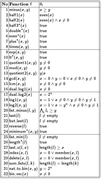
Our method proved successful on numerous examples (see Table 1 for some examples to illustrate its power). For each functionfin this table the correspond- ing termination predicate f could be synthesized automatically. Moreover, for all these examples the synthesized termination predicate is not only sucient for termination, but it even describes the exact domain of the functions.

These examples demonstrate that the procedure of Theorem 3 is able to synthesize sophisticated termination predicate algorithms (e.g. for a quotient algorithm it synthesizes the termination predicate \divides", for alogarithm al- gorithm it synthesizes a termination predicate which checks if one number is a power of another number, for an algorithm which deletes an element from a list a termination predicate for list membership is synthesized etc.). By subse- quent application of our simplication procedure one usually obtains very simple formulations of the synthesized termination predicate algorithms.

Termination of those algorithms marked with can be proved by methods for absolute termination proofs, too. But the termination behaviour of all other algorithms in Table 1 could not be analyzed with any other automatic method.

Although those functions without which have the termination predicate true are also total, their totality cannot be veried by the existing methods for ab- solute termination proofs. The reason is that their algorithms call other non- terminating algorithms. A detailed description of our experiments can be found in the appendix.

The presented procedure for the generation of termination predicates works for any given measure function^j:^j. Therefore the procedure can also be combined with methods for the automated generation of suitable measure functions (e.g.

the one we presented in [Gie95a, Gie95c]). For example, by using the measures suggested by this method, for all⁵ 82 algorithms from the database of [BM79]

our procedure synthesizes termination predicates which always returntrue(i.e. in this way (absolute) termination of all these algorithms is proved automatically).

Furthermore, with our approach it is also possible to perform termination

5As mentioned in [Wal94b] one algorithm (greatest.factor) must be slightly modied.

analysis forimperative programs: When translating an imperative program into a functional one, usually each while-loop is transformed into a partial function, cf. [Hen80]. Now the termination predicates for these partial \loop functions"

can be used to prove termination of the whole imperative program.

Acknowledgements.

We would like to thank Christoph Walther and the ref- erees for helpful comments.

No Function

^f f

1minus(x;y) xy 2half1(x) even(x)

3half2(x) even(x)^{^}x⁶=0 4half3(x) true

5double(x) true 6even(x) true 7plus(x;y) true 8times(x;y) true 9exp(x;y) true 10lt(x;y) true 11quotient1(x;y) y⁶=0 12mod(x;y) y⁶=0 13quotient2(x;y) y^jx

14gcd(x;y) x =0^{^}y =0^_x⁶=0^{^}y⁶=0 15lcm(x;y) x⁶=0^{^}y⁶=0

16dual log1(x) x⁶=0 17dual log2(x) x =2ⁿ

18log1(x;y) x =1^_x⁶=0^{^}y⁶=0^{^}y⁶=1 19log2(x;y) x =1^_x = y^{n^}x⁶=0^{^}y ⁶=1 20list minus(l;y) ^Vilⁱ y

21last(l) l⁶=empty 22but last(l) l⁶=empty 23reverse(l) true 24minimum(x;y)true 25list min(l) l⁶=empty 26length(l) true

27last x(l;x) length(l)x

28index(x;l) x =0^_member(x;l) 29delete(x;l) x =0^_member(x;l) 30sum lists(l;k) length(l) =length(k) 31nat to bin(x;y) y =2ⁿ

32bin vec(x) x⁶=0

Table 1.

Termination predicates synthesized by our method.

A Examples

This appendix contains 32 examples to illustrate the power of our method (cf.

Table 1). Algorithms marked with are (absolutely) terminating and only call terminating algorithms (they are required as auxiliary algorithms for the other examples). Hence their termination can also be proved with known techniques for absolute termination proofs. For all other algorithms in this appendix an automated termination analysis is not possible with methods for absolute ter- mination proofs. Note that in all following examples the termination predicates generated by our method are the weakest possible ones (i.e. they return true i the algorithm under consideration terminates).

For each algorithm we rst describe its intended semantics. Then we mention the termination predicate algorithm synthesized by our procedure (and the used measure function). Subsequently we show the results of applying the simplica- tion procedure to the termination predicate. This procedure always consists of the four steps:

(a) Induction Lemma,

(b) Subsumption Elimination, (c) Recursion Elimination, (d) Case Elimination.

After each of these four steps, we mention the intermediate version of the ter- mination predicate algorithm, where we omit steps that are not applicable in the particular example (and hence, do not change the termination predicate algorithm). In the end we describe the semantics of the resulting termination predicate.

The data structures used in the examples are nat (with the constructors 0 and succ and the selector pred) and list (with the constructors empty and add and the selectorsheadandtail). We omit termination predicates for constructors, selectors, and equality, because these predicates always return true.

1 minus

functionminus(x;y :nat) :nat⁽ if x = y then 0

else succ(minus(pred(x);y)) Intended Semantics:x y

Synthesis

Measure: m(x;y) =^jx^j#(i.e. the number of succ-applications in the rst argu- ment)

function minus(x;y :nat) :bool⁽ if x = y then true

else ^jpred(x)^j#<^jx^{j#^}minus(pred(x);y)

Simplication

(a) Induction Lemma

x⁶=0^!jpred(x)^j#<^jx^j# functionminus(x;y :nat) :bool ⁽

if x = y then true

else x⁶=0^{^}minus(pred(x);y) Semantics: xy

2 ^half1

function half1(x :nat) :nat⁽ if x =0 then 0

else succ(half1(minus(x;2))) Intended Semantics: x=2

Synthesis

Measure: m(x) =^jx^j#

function half1(x :nat) :bool⁽ if x =0 then true

else minus(x;2)^{^j}minus(x;2)^j#<^jx^{j#^}half1(minus(x;2))

Simplication

(a) Induction Lemma

minus(x;2)^!jminus(x;2)^j#<^jx^j# functionhalf1(x :nat) :bool⁽

if x =0 then true

else minus(x;2)^{^}half1(minus(x;2)) Semantics: true ix is even

3 half2

functionhalf2(x :nat) :nat⁽ if minus(x;2) =0 then 1

else succ(half2(minus(x;2))) Intended Semantics:x=2

Synthesis

Measure:m(x) =^jx^j#

functionhalf2(x :nat) :bool⁽ minus(x;2) ^{^} (if minus(x;2) =0

then true

else ^minus(^x;2)^{^j}minus(^x;2)^{j#<jxj#^}half2(minus(^x;2)))

Simplication

(a) Induction Lemma

minus(x;2)^!jminus(x;2)^j#<^jx^j# function half2(x :nat) : bool⁽

minus(x;2) ^{^} (if minus(x;2) =0 then true

else minus(x;2)^{^}half2(minus(x;2))) (b) Subsumption Elimination

minus(x;2)^!minus(x;2) function half2(x :nat) : bool⁽

minus(x;2) ^{^} (if minus(x;2) =0 then true

else half2(minus(x;2))) Semantics:true ix⁶=0andx is even

4 ^half3

functionhalf3(x :nat) :nat⁽

if x⁶=0^{^}x⁶=succ(0) then succ(half3(pred(pred(x)))) else 0

Intended Semantics:x=2