9 Horizontal heterogeneity
9.1 Simple two-surface systems
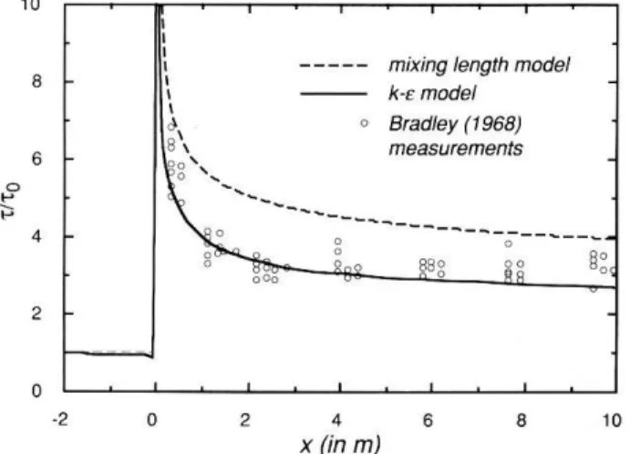
The simplest case of a surface heterogeneity consists of a sudden change in surface property, most ideally on a dividing line normal to the average flow direction. In this context the ‘surface property’ may be both, thermal or mechanical. On a very small scale the immediate change in the flow is emerging from the surface. For example, Fig. 9.1 shows the evolution of surface stress downwind of a step change in surface roughness with an immediate strong response and a more slowly developing relaxation towards a new equilibrium surface value. This new surface forcing is transported into the boundary layer aloft through turbulent transport resulting in modified profiles of mean variables (first order moments) or higher-order turbulence statistics. With increasing distance downwind of the step change a steadily growing layer emerges in which the profiles are in local equilibrium with the new surface. Within this layer the profiles are the same as they would be if the
‘new’ surface, i.e. the surface characteristics after the step change, had been the same for an infinite distance upstream. In terms of the footprint concept (see Chapter 8) this means that for any level within the equilibrium layer the entire footprint lies on the downwind side of the step change.
Figure 9.1 Comparison of modelled and measured surface shear stress after a smooth-to-rough transition, with M=125 (for the meaning of ‘M’ see eq.
(9.1), below). The ratio of the local shear stress to the smooth equilibrium value is plotted against the downwind distance. From Schmid and Bünzli (1995).
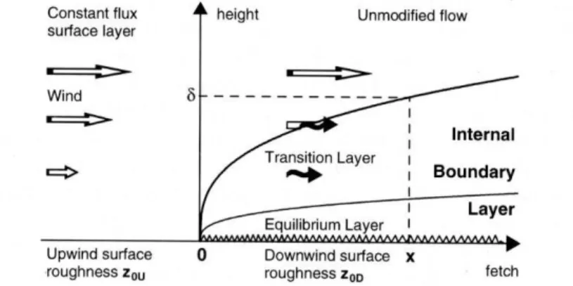
Above this equilibrium layer another layer evolves. It is the so-called internal boundary layer (IBL)1, within which the profiles are influenced by the change in surface conditions (Garratt 1992). It is sketched in Fig. 9.2. Its upper
1 More precisely, the Internal Boundary Layer contains the equilibrium layer. See Fig. 9.2.
boundary,
€
hIBL has been defined by Schliechting (1979; cited after Garratt 1992) as the height where the mean wind speed is essentially indistinguishable from the ‘free stream velocity’2, i.e.,
€
u =0.99u ∞. Again turning to the footprint picture, at the height
€
x3 =hIBL the entire footprint would lie on the surface upwind of the step change (Fig. 9.3).
Figure 9.2 Schematic of the Internal Boundary Layer. From Savelyev and Taylor (2005)
Figure 9.3 Schematic of the internal boundary layer evolving after a step change in surface roughness with the corresponding footprints at various levels.
The idealized picture of an internal boundary layer evolving after a step change in surface properties as outlined above calls for a number of specifications:
2 Apparently this concept stems from an idealized ‘wind tunnel world’ where the free stream velocity is clearly defined as the corresponding flow speed upstream of the step change. In the atmosphere it may exist only in very idealized situations.
If the IBL height were defined on the basis of variables other than the mean wind speed it would be different. For example if the stress would be used as a criterion (i.e.,
€
τ13 =0.99τ13,∞)
€
hIBL would be larger (at the same distance downwind of the change) since the turbulent exchange of higher order moments is more efficient than that of mean quantities.
The shape of the function
€
hIBL(x1), where
€
x1 is the distance downwind of the step change, is dependent on stability and also on the relative change of the surface property.
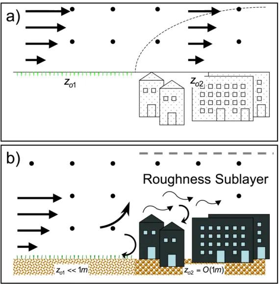
Most of our current knowledge on roughness changes stems from numerical modelling (e.g., Schmid and Bünzli 1995). It is common to all these studies that the surfaces each are characterised by a roughness length3. If one of the two surfaces considered is very rough such as an urban surface or a forest, the roughness sublayer (Section 8.3), which then covers a considerable part of the near-surface region (Fig. 8.7), would have to be taken into account (Fig. 9.4), but this only becomes feasible with increasing model resolution and LES modelling capabilities.
Excellent compilations of different formulations to determine
€
hIBL(x1) for various surface characteristics, together with a large number of references can be found in Garratt (1990, 1992) and Kaimal and Finnigan (1994). It is beyond the scope of this book to repeat them here. Rather the most salient features for typical situations will be outlined in the following sections.
3 In other words, the lowest model layer is assumed to possess SL properties and bluff body effects are not taken into account.
Figure 9.4 Illustration of modelled roughness change with very rough surfaces being involved. a) Traditional set-up where the surface roughness is characterized through the roughness length, and b) the ‘real’ situation, in which bluff body effects are effective (i.e., the model that is indicated through its black dot grid points needs to take into account roughness sublayer flow characteristics).
9.1.1 Roughness changes
Step changes in surface roughness are predominantly dependent on the magnitude of the change, which is usually expressed as
€
M=ln zo1 zo2
=ln(zo1)−ln(zo2), (9.1)
where the subscripts ‘1’ and ‘2’ refer to the surface upstream and downstream of the change, respectively. In this characterisation the smooth-to-rough transition results in
€
M<0 and the rough-to-smooth transition in
€
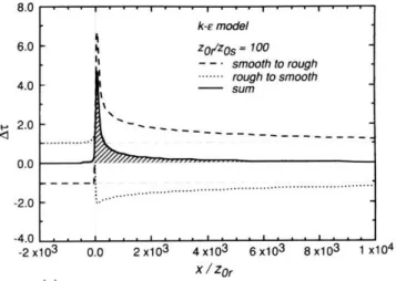
M >0. These two generic situations are fundamentally different in as the overshooting of the
surface stress response for the smooth-to-rough case is stronger than the corresponding ‘undershooting’ for the opposite situation. This can be seen from Fig. 9.5 where the variable
€
Δτ = τ − τa
τr −τa (9.2)
is displayed as a function of distance from the transition. Here,
€
τa =(τr +τs) / 2 is the average surface stress resulting from the (infinitely) rough (
€
τr) and smooth (
€
τs) surfaces, respectively. Note that in this representation
€
Δτ = +1 results for the rough surface and
€
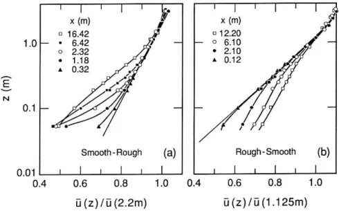
Δτ =−1 for the smooth surface. Figure 9.5 reveals that the difference in the surface stress response extends to a downwind distance of some few thousand roughness lengths4. Characteristic profiles of mean wind speed for the two cases are shown in Fig. 9.6. While the smooth-to-rough transition is accompanied with a slowing down of the flow due to increased friction the opposite is the case for the rough-to-smooth transition. For the large distances from the step change the semi-logarithmic plot of Fig. 9.6 also reveals the growing layer of equilibrium with the new surface (close to logarithmic wind profile for the near- neutral situation).
Figure 9.5 Numerical model results illustrating the asymmetry in the surface stress response after a step change in surface stress. Flow is from left to right. The hatched area reflects the difference between the smooth-to- rough (dashed line) and the rough-to-smooth (dotted line) cases.
Several approaches have been proposed for the description of the internal boundary layer height,
€
hIBL(x1). The one that is most often used originates on Panofsky and Dutton (1984) and is based on the assumption that the vertical diffusion [of the information on the changed surface] is proportional to the downwind friction velocity implying that for steady state conditions
€
∂hIBL/∂x1=Bu*2/u 1, where
€
B≈1.3 corresponds to the neutral limit of
€
σu3 /u*
4 In this case expressed as the roughness length from the rough surface of the two.
(eq. 4.26 - see Savelyev and Taylor 2001). Upon integration using the logarithmic wind profile over the downwind surface and with the boundary condition that
€
hIBL(x1=0)=zo2 we obtain an implicit relation for the internal boundary layer height
€
1+hIBL
zo2 ln(hIBL zo2)−1
= kB
zo2x1. (9.3)
Equation (9.3) has been tested against atmospheric data and found to perform quite well (Walmsley 1989) and, in particular, better than earlier, simpler models. Still, a prominent drawback was considered the fact that the upstream surface and hence the turbulence state of the boundary layer approaching the step change is not considered in this model. Also the character of the change (rough-to-smooth or vice versa) cannot be taken into account through (9.3). Savelyev and Taylor (2001) have offered a reconsideration and basically argue that i) the upwind surface determines the conditions into which the new internal boundary layer has to grow and ii) the roughness change (
€
M) may empirically be taken into account. They propose a slightly modified, but again implicit relation according to
€
hIBL
zo1 ln(hIBL zo1)−1
= BkAN
zo1 x1, (9.4)
where
€
AN =1−0.1M is an empirically obtained function to express the neutral (subscript ‘N’) proportionality constant’s dependence on the roughness change5. Savelyev and Taylor (2001) show that their revised formulation yields slightly better results than (9.3) for the atmospheric data under consideration (Fig. 9.7). These data sets were all from relatively moderate changes in surface roughness (
€
M= ±5.7). It may be assumed that for a ‘more extreme’ case such as a transition from sea surface to a city, equation (9.4) would be better to account for the roughness change. Savelyev and Taylor (2005) have slightly modified their analysis of 2001 (i.e., eq. 9.4) by taking additional processes into account, which might affect the upward propagation of information from the new (downwind) surface (see their paper for details).
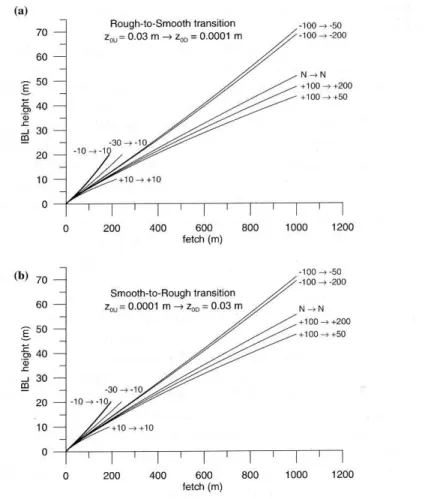
Moreover they have extended the analysis to non-neutral conditions. For this they assume, in addition to the roughness change, one in surface sensible and latent heat fluxes, that is expressed in terms of the Obukhov lengths for the upwind and the downwind surfaces, respectively. Rather than reproducing their quite involved implicit expression and the corresponding approach to find a solution, Fig. 9.8 shows numerical results for various roughness-plus- stability step changes. Overall, Fig. 9.8 reveals that the more unstable the upwind flow is, the faster the IBL grows. Most importantly, when comparing the two panels in Fig. 9.8 it can be seen that the influence of stability dominates over the roughness change. Thus in a generally unstable
5 Note that we have defined the roughness change (9.1) in reversed order than Savelyev and Taylor (2001). Also, in their original paper, an integration constant appears that eventually is set to zero as a convenient and simple choice.
environment the IBL growth is faster than in a neutral or stable environment. If stability is allowed to change sign over the roughness change (not shown), it appears that the upwind stability dominates the picture, but not symmetrically around the neutral stratification. Savelyev and Talyor (2005) offer some limited experimental evidence to support their extension to non-neutral flows but a more comprehensive comparison to field data will be needed.
Figure 9.6 Development of logarithmic velocity profiles at different distances after a roughness change, a) smooth-to-rough and b) rough-to-smooth.
From Kaimal and Finnigan (1992).
Figure 9.7 IBL height (m) – here denoted as
€
δ: calculated from Eq (9.4) vs.
observed, atmospheric data. Data symbols according to Walmsley (1989). From Savelyev and Taylor (2001).
Figure 9.8 IBL height growth for non-neutral conditions, a) rough-to-smooth and b) smooth-to-rough. The numbers near the curves denote the value of the Obukhov length upwinddownwind of the roughness change, N indicates neutrality. Curves are drawn up to a height that limits the underlying assumptions. From Savelyev and Taylor (2005).
9.1.2 Thermal internal boundary layers
The most prominent example of a step change in thermal surface properties can be found at the shore where the sea (or lake) surface temperature remains relatively constant throughout the day while the land surface may undergo large changes due to the daily cycle of net radiation. Moreover, under weak synoptic conditions this situation leads to the formation of a sea breeze (flow from the sea towards the land) during the day6 and vice versa during the night. Thus the flow is indeed often directed perpendicular to the shoreline.
As for the change-in-roughness case, models for the internal boundary layer growth of varying sophistication exist. The simplest is probably a steady state, purely advective situation with a horizontally homogeneous surface heating.
Garratt (1992) shows that in this simplified situation the thermal internal
6 Essentially, the heated land surface exhibits a lower pressure thus leading to a local circulation system with on-shore flow near the surface and a reversed flow aloft.
boundary layer (TIBL) grows proportionally to the square root of the distance from the surface discontinuity
€
hTIBL =ax1/ 2, (9.5)
where
€
a, the proportionality factor depends on the (uniform) surface heat flux over the heated land surface, the average wind speed in the TIBL and the gradient of potential temperature above the TIBL. For reasonable values of these variables,
€
a is on the order 10 (see Garratt 1992 for details).
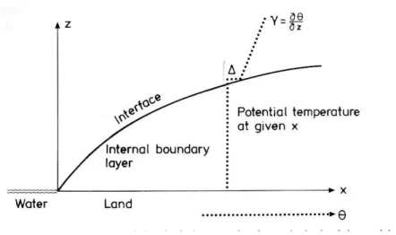
Gryning and Batchvarova (1990) present a model for a situation that is somewhat less idealised (Fig. 9.9). In particular, they take into account the temporal development of the inversion strength (
€
Δ). Similar concepts are employed for the description of the temporal development of the ML (e.g.
Seibert et al 2000). Their idealisation consists in a restriction to a stably stratified (upwind) boundary layer over the water.
Figure 9.9 Schematic illustration of the physical basis for the model of Gryning and Batchvarova (1990).
Gryning and Batchvarova (1990) derive a prediction equation for
€
hTIBL as a function of downwind distance from the coastline based on an idealised conservation equation of heat (steady state, no internal sources or sinks)
€
∂(u 1θ )
∂x1 +∂(u 3θ )
∂x3 =−∂u'3θ'
∂x3 (9.6)
and the (two-dimensional,
€
x1, x3) continuity equation (5.8). Integrating (9.6) from
€
x3 =0 to
€
hTIBL(x1) and using the continuity equation to obtain
€
u 3(x3 =hTIBL) as a boundary condition yields (see the original paper for a lengthy derivation)
€
dθhTIBL dx1 u 1
0 hTIBL
∫ dx3 =u'3θ'o−u'3θ'h
TIBL. (9.7)
The potential temperature at the height of the internal boundary layer can be seen from Fig. 9.9 to be
€
θhTIBL =γhTIBL − Δ+const. (9.8)
To solve (9.7), (9.8) must first be differentiated with respect to
€
x1:
€
dθ hTIBL
dx1 =γ dhTIBL
dx1 −∂Δ(hTIBL)
∂hTIBL
dhTIBL
dx1 . (9.9)
Thus the rate of change of the inversion strength
€
Δ with respect to the height of the TIBL must be known. For this the starting point is a description of the (downward) turbulent heat flux at the top of the growing boundary layer relating it to the entrainment rate
€
dhTIBL /dt
€
−u'3θ'hTIBL =ΔdhTIBL
dt . (9.10)
€
Δ decreases through heating of the internal boundary layer,
€
dθTIBL/dt, on the one hand and increases due to growth of the TIBL into the stable layer above:
€
dΔ/dt =γ dhTIBL
dt −dθTIBL
dt , (9.11)
where
€
γis the gradient of potential temperature above the TIBL (Fig. 9.9). The heating rate of the TIBL (recall Fig. 9.9, i.e. constant potential temperature throughout the TIBL in this approximation) is given as
€
dθTIBL
dt =u'3θ'o/hTIBL−u'3θ'h
TIBL /hTIBL. (9.12)
Substituting (9.12) and (9.10) into (9.11) yields
€
(hTIBL dΔ
dhTIBL +Δ −γhTIBL)dhTIBL
dt =−u'3θ'o. (9.13)
Again using (9.10) for
€
dhTIBL /dtand using an idealised TKE budget equation for the entrainment zone (Tennekes and Driedonks 1981)
€
−u'3θ'h
TIBL =Au'3θ'o+Bu*3θTIBL /ghTIBL, (9.14) equation (9.13) can be expressed as
€
dΔ
dhTIBL +Δ( 1
hTIBL + 1
AhTIBL −BκL)=γ, (9.15)
where the definition of the Obukhov length (4.12) has been used. In (9.14),
€
Au'3θ'o accounts for thermal and
€
Bu*3θTIBL /ghTIBL for mechanical turbulence.
€
A≈0.2 and
€
B≈2.5 are often used for the parameters (but see the discussion in Gryning and Batchvarova 1990 and Seibert et al. 2000). Equation (9.15) can be integrated fully (Gryning and Batchvarova 1990) and a (more convenient) approximation reads
- 11 -
€
Δ
γhTIBL = AhTIBL −BκL
(1+2A)hTIBL −2BκL. (9.16)
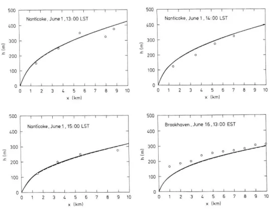
Figure 9.10 Comparison of simulated and observed IBL heights for some experiments, from Gryning and Batchvarova (1990).
To re-formulate (9.7), (9.9) is used along with (9.15) and (9.16) to yield
€
γ( (1+A)hTIBL −BκL
(1+2A)hTIBL −2BκL) 0 u 1dx3 hTIBL
∫
dhTIBL
dx1 =u'3θ'o−u'3θ'hTIBL (9.17) For the integral in (9.17) Gryning and Batchvarova (1990) use similarity theory (with some reservation) to yield
€
u 1dx3
0 hTIBL
∫ =[u 1(hTIBL)−R(hTIBL/L)u*]hTIBL, (9.18) where the function
€
R(hTIBL/L) is, in their final solution, found to be rather weak and eventually set to a constant. The analytical solution to (9.17) is called by the authors ‘rather unattractive’. Instead they provide an approximate solution according to
(u 1(hTIBL)−Ru*) C1
hTIBL2 2 +2C2
C1 hTIBL+(2C2
C1 )2ln − C1
2C2hTIBL+1
+ Bu*2u 1θTIBL
Cγg(1+A)ln −(1+A)
C2 hTIBL +1
= u'3θ'o γ x1.
(9.19)
Here, C=1.3;
€
C1=1+2A and
€
C2=BκL are abbreviations. The derivation shows that the combined effects of thermal and mechanical turbulence in this problem of internal boundary layer growth does not allow for a ‘simple treatment’ – even if some idealisations are invoked. The implicit solution for
€
hTIBLin (9.19) is shown in Fig. 9.10 to favourably correspond to observations.
9.2 Heterogeneous Surfaces
In reality surfaces are most often neither homogeneous nor of the simple ‘A-B type’ as considered in section 9.1 (see, for example Fig. 8.2). Still,
‘horizontally averaged surface fluxes’ are often needed, as for example in numerical models where a ‘grid point’ is in fact representing and area of
€
Δx2 (where
€
Δx is the side length of a grid box). A natural approach would consist in trying to find the average (or ‘effective’) flux from relating the mean (i.e., grid-average) variable at the first model level to the surface by using similarity theory (see Fig. 5.2 for an illustration). For momentum under neutral conditions this would be the ‘logarithmic wind profile’ (eq. 4.16) and hence an
‘effective roughness length’ is required to characterise the heterogeneous surface. However, two basic questions arise: 1) how high does the ‘first model level’ to be in order to allow for employing such an effective flux concept and 2) how can the non-linearity of surface information (such as the roughness length) be taken into account? The next sub-sections try to elucidate some of the concepts often used in addressing these questions.
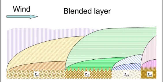
9.2.1 Blending height and effective fluxes
Based on theoretical considerations Mason (1988) proposed the concept of a blending height as the height, at which turbulent mixing would have blended the internal boundary layers at each transition from one surface type to another into an ‘equilibrium or blended layer’, wherein the flow is independent of horizontal position (i.e., representing the area-averaged conditions). Figure 9.11 schematically shows such a situation. For the existence of a blending height with respect to momentum exchange, Mason (1988) argued that i) an equilibrium layer must exist close to the surface where MOST applies and ii) above the blending height a logarithmic wind profile (for neutral conditions) exists. Hence, the mean wind speed in the blended layer (‘B’) obeys
€
<u1,B >= <τ13,eff >
k ln(x3,B
zo,eff) (9.20)
with the angular brackets denoting spatial averages. Various considerations exist to determine effective roughness lengths (see for example references listed in Schmid and Bünzli 1995). Here it is only important to note that the effective roughness length is always larger than a simple area average (up to a factor of ten or so) due to local advection. Hasager and Jensen (1999) have devised a sophisticated (but cost effective) numerical sub-grid scale model that allows for taking into account arbitrarily distributed surface patches for the determination of effective roughness lengths. Hasager et al (2003) have further expanded the method to the use of satellite-derived land cover maps.
An extension of the concept to scalar fluxes can be found in Wood and Mason (1991).
Figure 9.11 Conceptual sketch of a blending layer evolving over surface patches with different roughnesses.
The blending height has been estimated by Mason (1988) to be on the order of
€
Lx/ 200, where
€
Lx corresponds to the characteristic horizontal length scale of the roughness change (i.e., the ‘average’ distance between different roughness patches). However, it is clear that in principle the blending height must also be dependent on the (individual) roughness lengths considered (Bou-Zeid et al 2004). In connection with numerical modelling, the blending height and associated effective flux (effective roughness) concepts would demand the first model level to be above the blending height. However, the basic assumption in Mason’s heuristic approach for the blending height (applicability of MOST close to the surface over the individual patch, see above) restricts this estimate to moderate roughness lengths over which no distinguishable Roughness Sublayer (Section 8.3 and Chapter 10) exists. For the estimation of the blending height in the case of a surface consisting of different (very) rough surfaces, as for example in a city with different quarters, roughness sublayer effects would have to be taken into account.
9.2.2 Mosaic approach and tiles
Another approach that responds to the problem of sub-grid scale heterogeneity of surface properties in numerical models is the so-called Mosaic Approach (Seth et al 1994; Amendt 2006). Again it recognises that the effective (grid averaged) flux of momentum, energy or mass is not simply an average, but rather modified through local advection. Therefore, the surface exchange calculation in a numerical model is performed at a higher spatial resolution (Fig. 9.12). Still, due to excessive increase of computing time, the
high resolution is only employed for the surface exchange. Figure 9.13 shows a comparison between observed and modelled area-averaged surfaces fluxes in the area of the Lindenberg observatory in Germany during the so-called LITFASS experiment (Beyrich et al. 2006). Clearly, the surface energy fluxes from the coarse resolution simulation (21 km in this example – encompassing in one grid cell more or less the entire experimental area) exhibit a systematic bias as compared to the high-resolution simulations. In the Mosaic approach it is in principle only the resolution of the calculated surface exchange that limits the accuracy of the results. This can be seen from Fig 9.14 where the surface latent heat flux pattern is depicted from a coarse resolution simulation with Mosaic, compared to a (very costly) high-resolution simulation.
Figure 9.12 Schematic of the ‘Mosaic approach’ for taking into account sub-grid scale surface heterogeneity in meso-scale numerical models (courtesy Felix Ament).
A variant of the mosaic approach consists of determining the area fraction of each surface type in the (coarse resolution) grid box. For each of these so- called tiles the surface fluxes are then determined individually and a weighted average finally yields the fluxes for the box. Clearly, in this Tiles Approach the details of the local advection processes are neglected but computing time can be saved if small patches of the same surface type are present within a given grid cell. Figure 9.13 reveals that the results are comparable to the Mosaic approach if the distribution of surface types is not particularly ordered.
Figure 9.13 Average surface energy fluxes from nine ‘golden days’ during the LITFASS-2003 experiment (Beyrich et al. 2006) at the Lindenberg Observatory in Germany. ‘Obs’ = observations from 14 sites (=’LITFASS area mean’), ‘LM’ refers to the ‘Local Model’ of the COSMO Consortium (Steppeler et al 2003) with the respective numbers indicating the horizontal resolution (in km). Various variants indicated by letters. From Ament (2006)
Figure 9.14 Comparison of surface latent heat flux patterns during the LITFASS- 2003 experiment (Beyrich et al. 2006), Case study, 30 May 2003, 12 UTC. Left: LM run with 7 km horizontal resolution with Mosaic invoked, right: high—resolution (1 km) reference. From Ament (2006)
References Chapter 9
Ament F: 2006, Energy and moisture exchange processes over heterogeneous land-surfaces in a weather prediction model, PhD Thesis, Rheinische Friedrich-Wilhelms-Universität Bonn, 137pp.
Beyrich F, Leps JP, Weisensee U, Bange J, Zittel P, Huneke S, Lohse H, Mengelkamp HT, Foken T, Mauder M, Bernhofer C, Queck R, Meijninger WML, Kohsiek W, Lüdi A, Peters G, and Münster H: 2006, Area averaged surface fluxes over the heterogeneous LITFASS area from measurements, Boundary-Layer Meteor. in revision.
Bou-Zeid E, Meneveau C, Parlange MB: 2004, Large-eddy simulation of neutral atmospheric boundary layer flow over heterogeneous surfaces: Blending height and effective surface roughness, Water Resources Res, 40, W02505, doi:10.1029/2003WR002475.
Garratt JR: 1990, The internal boundary layer – a review, Boundary-Layer Meteorol, 50, 171- 203.
Garratt JR: 1992, The atmospheric boundary layer, Cambridge University Press, 316pp.
Gryning S-E and Batchvarova E: 1990, Analytical model for the growth of the coastal internal boundary layer during onshore flow, Quart J Royal Meteorol Soc, 116, 187-203.
Hasager CB and Jensen NO: 1999, Surface-flux aggregation in heterogeneous terrain, Quart J Royal Meteorol Soc, 125, 2075-2102.
Hasager CB, Nielsen NW, Jensen NO, Boegh E, Chritiansen JH, Dellwik E and Soegaard H:
2003, Effective roughness calculated from satellite-derived land cover maps and hedge information used in a weather forecasting model, Boundary-Layer Meteorol, 109, 227- 254.
Kaimal JC and Finnigan JJ: 1994, Atmospheric Boundary Layer Flows, Oxford University Press, New York, 289pp.
Mason PJ: 1988, The formation of areally-averaged roughness lengths, Quart J Royal Meteorol Soc, 114, 399-420.
Panofsky HA and Dutton JA: 1984, Atmospheric Turbulence, John Wiley & Sons, New York, 397 pp
Savelyev SA and Taylor PA: 2001, Notes on an internal boundary-layer height formula, Boundary-Layer Meteorol, 101, 293–301.
Savelyev SA and Taylor PA: 2005, Internal boundary layers:I. Height formulae for neutral and diabatic flows, Boundary-Layer Meteorol, 115, 1-25.
Schmid HP and Bünzli D: 1995, The influence of surface texture on the effective roughness length, Quart J Roy Meteorol soc, 121, 1-21.
Seibert P, Beyrich F, Gryning S-E, Joffre S, Rasmussen A and Tercier P: 2000, Review and intercomparison of operational methods for the determination of the mixing height, Atm Environ, 34, 1001-1027.
Steppeler J, Doms G, Schattler U, Bitzer HW, Gassmann A, Damrath U, Gregoric G: 2003, Meso-gamma scale forecasts using the nonhydrostatic model LM, Meteorology Atmos Phys, 82 (1-4), 75-96.
Tennekes H and Drriedonks AGM: 1981, Basic entrainment equations for the atmospheric boundary layer, Boundary-Layer Meteorol, 20, 515-531.
Walmsley JL: 1989, Internal Boundary-Layer Height Formulae - A Comparison with Atmospheric Data, Boundary-Layer Meteorol., 47, 251-262.
Wood N and Mason P: 1991, The influence of statit stability on the effective roughness lengths for momentum and heat transfer, Quart J Royal Meteorol Soc, 117, 1025-1056.