Worksheet 5 Long range interactions: Direct sum and Ewald summation

Simulation Methods in Physics II (SS 2014)

Worksheet 5

Long range interactions: Direct sum and Ewald summation

Jens Smiatek

and Christian Holm

June 13, 2014 ICP, Uni Stuttgart

Important remarks

•

Due date:

•

You can send a PDF file to Anand Narayanan Krishnamoorthy (anand@icp.uni-stuttgart.de) or submit a hand-written copy.

•

If you have further questions, contact Jens Smiatek (smiatek@icp.uni-stuttgart.de) or Anand Narayanan Krishnamoorthy (anand@icp.uni-stuttgart.de).

1 Introduction

This tutorial is intended to strengthen your knowledge on long range interactions. As you have learned in previous lectures, special techniques are needed to deal with long-range interactions in a proper way. Simple truncation of the long-range forces usually ends up in a substantial and unwanted modification of the physics of a problem. In order to do the tutorial you have to use the additional material coming together with this work sheet within a zip-file. You will find there a set of folders containing the programs needed for each section.

2 The direct sum

Periodic boundary conditions are frequently used in order to approach bulk systems within the limits of currently available computers. We will consider a main cell which is surrounded by

∗smiatek@icp.uni-stuttgart.de

†holm@icp.uni-stuttgart.de

replica cells that fill the whole space. The main cell consists of N particles with charges q

at position r

in a cubic box of length L. Our objective is to compute the energy U associated to the main cell. The energy U is due to the Coulomb interaction of the particles located inside the main cell with other particles present in the cell, as well as with the particles located in the replica cells. The energy of the main cell in this PBC system is

U = 1 4πǫ

1 2

N

X

i=1 N

X

j=1

†

X

n∈Z³

q

q

rij

+ n

(1)

where

=

. The sum over n is over all simple cubic lattice points, n = (n

L, n

L, n

L) with n

, n

and n

integers. The

indicates that the i = j term must by omitted for n = 0 to avoid to take into account the interaction of a particle with itself. Equation 1 is only conditionally convergent in 3D. In other words, the value of the sum is not well defined unless one specifies the way we are going to sum up the terms (spheric, cubic, cylindric, etc.). An explanation from a more physical point of view about the conditional convergence of eq. 1 lies in the fact that we have an infinitely large system, that although is useful for our purposes of mimicking the bulk, it is never found in physical cases. When we perform an order summation, we are distributing the cells (the charges) in the space in a certain way. If we perform two different order summations, we will get two different values of the interaction because we have two different charge distributions. One could think that as farther the replica boxes are from the main cell, less important should be their contribution. This is the case for single cells, but the number of cells grows in such a way that always there is a finite contribution from the cells placed at a certain large distance from the main cell. The use of eq. 1 in order to compute electrostatic magnitudes is know as

The direct sum method, although simple to implement, suffers from a major drawback: the numerical evaluation of eq. 1 is excessively computer demanding. The first thing one can notice in eq. 1 is that the sum over n is an infinite series because it runs over all

. This entails that when we want to evaluate the sum numerically we must perform a cut-off, i.e., we assume that the contributions arising from larger n values can be neglected. Usually one chooses to perform a spherical sum, i.e., we take into account only the terms that satisfy

< n

.

The introduction of a cut-off implies that we are going to do an error when we compute eq. 1

numerically. If we increase n

, we will get a more accurate value of U ,

to a certain value. In principle, the introduction of a cut-off is not a problem, because for practical

purposes we are never in the need of an infinitely accurate result. Nonetheless, in practice, the

use of the direct sum method requires of a large cut-off to get results accurate enough to be used

in simulations. Furthermore, when we increase n

, the number of cells to take into account

scales as n

and not linearly because n is a 3D vector. If we assume that the time we need to

compute the sum is proportional to the square of the number of particles we have in the extended

system (main cell + replicated cells), then the computer time we need scales as n

N

, where

N is the number of particles we have in the main cell box. Therefore, in general, the direct

sum method is of little use for simulations, although it is very useful tool to test the correctness

of more advanced methods. Notice, that in order to use a direct sum code to test the output of

other more sophisticate programs, it would be desirable that we have previously checked the

correctness of the direct sum code. But, how to that?

An easy test we can perform is the numerical evaluation of the Madelung’s Constant for a certain crystal structure.The value of the Madelung’s constant can be evaluated analytically up to a very high accuracy and it is easy to find it tabulated. The Madelung’s constant depends on the geometric arrangement of the ions in the crystal structure, and it is particular for each type of crystal structure. For simple ionic crystal’s like NaCl it can be related to the energy of an ion

U

= M

q

4πǫR (2)

where q is the absolute value of the charge of the ions and R the distance between two nearest neighbours. M

is the Madelung’s constant

M

=

i

X

j

sign(q

q

) R r

(3)

where sign(q

q

) is depending on the sign of the product q

q

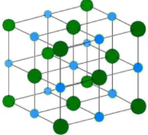
. In the case of a NaCl-crystal (see structure in figure 1), the value of the Madelung constant is

M

=

1.7475645946331821906362120355443974034851614366247417581528253507 . . . .

Figure 1: The crystal structure of NaCl. Taken from

Tasks: (6 points)

1. Using the direct sum method, evaluate the Madelung’s constant for a NaCl crystal. Hint:

in the folder problem_1 you will find a program that performs direct sums. At least two errors have been introduced on purpose on the code.

2. Using the linux command gprof, check which is the scaling of time with the cutoff n

. Hint: you must compile the code including the -pg flag. Run the program, and then execute gprof name-executable > report-file. Justify the result.

3. Is it correct to cutoff the long-range interactions in simulations? Justify the answer in

terms of the results you have obtained in the previous tasks for the Madelung’s constant.

3 The Ewald sum

Ewald summation is a faster method to compute electrostatic quantities such as energies or forces. The Ewald sum is based on splitting the slowly convergent equation 1 into two series which can be computed much faster (at a level of fixed accuracy). The trick basically consists of splitting the interaction 1/r as

1

r = f (r)

r

1

f (r)

r (4)

where the usual choice is f (r) = erf c(αr), where α is called the Ewald splitting parameter, which results in the well known Ewald formula for the energy of the main cell

U = U

+ U

+ U

+ U

(5)

where U

is called the real space contribution, U

is the reciprocal space contribution, U

is the self-energy, and U

accounts for the dipolar correction as they have been also introduced for a spherical sum in the lecture. The explicit expressions are given by

U

= 1 2

N

X

i=1 N

X

j=1

†

X

n∈Z³

q

q

erf c(α

+

L

)

|rij

+

L

(6)

U

= 1 2L

X

k∈K³,k6=0

4π

k

exp(

k

/4α

)

N

X

i N

X

j

q

q

exp(

ikr

) (7)

U

=

α

√

π

N

X

i

q

(8)

and

U

= 2π (1 + 2ǫ

)L

N

X

i

q

r

!2

(9) where ǫ

is the dielectric constant, and

=

2π

/L :

. In practice the sums for U

and U

are evaluated performing cutoffs given by r

and k

. Typical implementations, as the one we are going to use, assume the minimum image convention, i.e., r

< L/2 and therefore

= 0 in the expression for U

.

Tasks: (4 points)

1. In the folder problem_2 there is a code in which Ewald sum is implemented using the minimum image convention. Set the values r

= 3, k

= 7, and use the code to analyse how the estimate of the Madelung constant we obtain depends on the value of the Ewald splitting parameter α (study the cases α

[0.1, 2]. Which conclusions do you extract from the previous results? Is the value of the estimate for the Madelung constant dependent of the parameter α? Does it depend on the values chosen for r

and k

? What happens if we increase r

and k

? Which are the best values of α, r

and k

to get the Madelung Constant faster with an accuracy no less than 10

?

2. Why the values we obtain depend on α, r

and k

? What is the origin of the errors we

observe when we evaluate the Ewald sum? Justify the answer.

4 Error estimates

As you have noticed in the previous task, we can obtain in a short time very accurate values for the Madelung’s constant of the NaCl for certain values of the parameters α, r

, and k

. Unfortunately it is not straightforward to obtain an optimal set of values for α, r

, and k

. In general, given a certain required accuracy level, we would like to be able to analytical predict which is the error we have for a given set of these parameters. Fortunately, such error estimates for Ewald sums were developed in the 90’s by Kolafa and Perram (Mol. Sim.,

with

δU

= Q

(r

/2L

)

(αr

)

exp(

α

r

) (10) and

δU

= Q

απ

k

exp(

(πk

/αL)

). (11)

1. The same code in the folder problem_2 that we used in the previous task contains a sub- routine that implements the previous errors. Furthermore, the subroutine is able to seek for the optimal parameters α, r

, and k

to use when a certain given accuracy level is specified. To make use of this subroutine, uncomment in the code the four lines labelled as U N COM M EN T . Using this modified code, check how close are the parameters you have obtained in the previous task to to the optimal parameters (Madelung Constant with an accuracy no less than 10

).

2. If we want to compute the Madelung’s constant of the NaCl, with an accuracy of 10

, which method is faster, the direct sum or the Ewald sum? Can you obtain an accuracy of 10

using the direct sum program? In case you can’t, try to infer which is the root of the problem? Hint: Try to reduce or increase the length L of the system, and see what occurs with the accuracy.

3. If we want to compute the energy of a system of 100 randomly positioned particles, in a box of size L = 10, with an accuracy of 10

, which method is faster, the direct sum or the Ewald sum?

5 The P

M method

Although the Ewald sum method represents a substantial improvement with respect to the direct

sum, in many cases it is not as fast as we would like. This drawback is specially notorious when

we are dealing with systems containing a large number of particles. The problem is mainly due

to the fact that the computer time in Ewald sums scales with the number of particles as N

, or

in the best versions as N

. These exponents entail that the computer time grows very quickly

with the number of particles. A faster algorithm that scales like N log(N )

N is the P

M

method (particle-particle-particle mesh). The trick used in P

M consists on the evaluation of

the implicit Fourier Trans- form present in U

through the use of the so-called Fast Fourier

Transforms (FFT), which reduce substantially the time needed to compute the reciprocal space

contribution U

.

1. In the folder problem_3 you will find a script for executing P

M by using the software package

. Try to understand what the code is doing. Notice specially the command inter coulomb. Ask the instructor if you have doubts about the use or function of any of the commands in the script. Compute the Madelung’s constant with an accuracy of 10

by using Espresso.

2. Now we have acquired practice on the use of Direct Sum, Ewald Sum and P 3M methods,

let’s use them to evaluate the energy of a neutral system of 500 charges randomly located

inside a system of size L = 30, with an accuracy of 10

. Check that the three different

methods agree on the result. Which method is faster?