Cell Model and Poisson-Boltzmann Theory: A Brief Introduction

Cell Model and Poisson-Boltzmann Theory: A Brief Introduction

Article · January 2002

DOI: 10.1007/978-94-010-0577-7_2 · Source: arXiv

CITATIONS

26

READS

73

2 authors, including:

Markus Deserno Carnegie Mellon University 116PUBLICATIONS   4,819CITATIONS   

SEE PROFILE

All content following this page was uploaded by Markus Deserno on 04 May 2014.

The user has requested enhancement of the downloaded file.

arXiv:cond-mat/0112096v1 [cond-mat.soft] 6 Dec 2001

A BRIEF INTRODUCTION

MARKUS DESERNO¹,CHRISTIAN HOLM²

1 Department of Chemistry and Biochemistry, UCLA, USA

2 Max-Planck-Institut f¨ur Polymerforschung, Mainz, Germany Email: ¹markus@chem.ucla.edu,²holm@mpip-mainz.mpg.de

The cell-model and its treatment on the Poisson-Boltzmann level are two important concepts in the theoretical description of charged macro- molecules. In this brief contribution to Ref. [1] we provide an introduction to both ideas and summarize a few important results which can be obtained from them. Our article is organized as follows: Section 1 outlines the se- quence of approximations which ultimately lead to the cell-model. Section 2 is devoted to two exact results, namely, an expression for the osmotic pres- sure and a formula for the ion density at the surface of the macromolecule, known as the contact value theorem. Section 3 provides a derivation of the Poisson-Boltzmann equation from a variational principle and the assump- tion of a product state. Section 4 applies Poisson-Boltzmann theory to the cell-model of linear polyelectrolytes. In particular, the behavior of the exact solution in the limit of zero density is compared to the concept of Manning condensation. Finally, Section 5 shows how a system described by a cell model can be coupled to a salt reservoir, i. e., how the so-called Donnan equilibrium is established.

Our main motivation is to compile in a concise form a few of the basic concepts which form the arena for more advanced theories, treated in other lectures of this volume. Many of the basic concepts are discussed at greater length in a review article by Katchalsky [2], which we warmly recommend.

1. The cell model

1.1. THE NEED FOR APPROXIMATIONS

Solutions of charged macromolecules are tremendously complicated phys-

ical systems, and their theoretical treatment from an “ab initio” point of

view is surely out of question. The standard solvent itself – water – al-

ready poses formidable problems. Adding the solute requires additional understanding of the solvent-solute interaction, the degree of dissociation of counterions, the conformation of the macroions, its intricate coupling with the distribution of the counterions and many further complications.

How can one ever hope to achieve even some qualitative predictions about such systems?

Many of the interesting features of polyelectrolytes are ultimately a con- sequence of the presence of charges. One may thus hope that a theoretical description focusing entirely on a good treatment of the electrostatics and using crude approximations for essentially all other problems will unveil why these systems behave the way they do. In a first important step any quantum mechanical effects are ignored by using a classical description. A second simplification is to treat the solvent as a dielectric continuum and consider explicitly only the objects having a monopole moment. This “di- electric approximation” is motivated by the long-range nature of Coulomb’s law and works surprisingly well [3]. Since a classical system of point charges having both signs is unstable against collapse, a short-range repulsive in- teraction is required, which is most commonly modeled as a hard core. For a simple electrolyte this approximation is called the “restricted primitive model”.

In 1923 Debye and H¨ uckel studied such a system using the linearized Poisson-Boltzmann theory [4]. Their treatment accounted for the fact that ions tend to surround themselves by ions of opposite charge, which reduces the electric field of the central ion when viewed from a distance. While the exponentially screened Coulomb potential is one of the most prominent results, it must be noted that the authors computed the free energy of the electrolyte. Its electrostatic contribution scales as the 3/2 power of the salt density, which explains why a virial expansion must fail. A good textbook account is given in Ref. [5].

Though approximate, Debye-H¨ uckel-theory works very well for 1:1 elec- trolytes. However, perceptible deviations are already much larger in the 1:2 case. This is not merely a consequence of the presence of multivalent ions, namely that the increased strength of electrostatic interaction may corre- late ions more strongly. Rather, the

asymmetry

of the situation itself is a key source of the problem – see Kjellander’s lecture for more details [6].

It is for this very reason that in the highly asymmetric case of a charged

macromolecule surrounded by small counterions the standard Debye-H¨ uckel

theory cannot be applied.

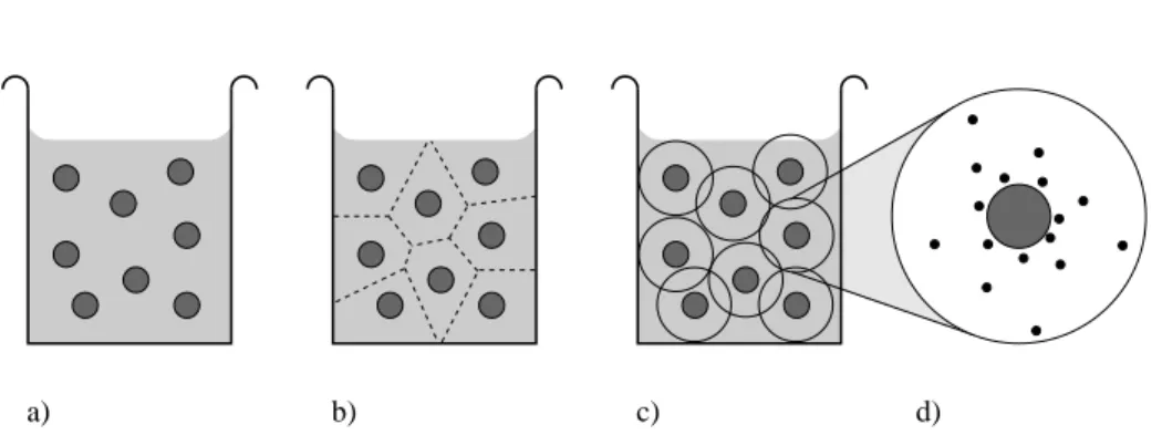
a) b) c) d)

Figure 1. Approximation stages of the cell model. The full solution (a) is par- titioned into cells (b), which are conveniently symmetrized (c). Subsequently the attention is restricted to just one such cell (d) and the counterion distribution within it.

1.2. DECOUPLING THE MACROIONS

The cell model is an attempt to turn this situation into an advantage: If the situation is highly asymmetric, there is no reason to pursue a symmet- ric treatment. Since the macroions all have the same charge, their mutual pair interaction is repulsive. Unless there are effects which cause them to attract, aggregate and ultimately fall out of solution, i. e., unless the effec- tive pair potential is no longer repulsive, the macroions will organize so as to keep themselves as far apart as possible. The total solution can now be partitioned into cells, each containing one macroion, the right amount of counterions to render the cell neutral, and possibly salt molecules as well.

As a consequence of the assumed homogeneous distribution of macroions, these cells will all have essentially the same volume, equal to the total vol- ume divided by the number of macroions. Observe that different cells do not have strong electrostatic interactions, since they are neutral by con- struction.

The cell model approximation consists in restricting the theoretical de- scription of the total system to just one cell. While the interactions be- tween the small ions with “their” macroion as well as with small ions in the same cell are explicitly taken into account, all interactions across the cell boundary are neglected. Note that the existence of cells, all of which have essentially the same size, requires correlations to be present between the macroions. However, these correlations are no longer the subject of study.

The cell model can thus be viewed as an approximate attempt to factorize the partition function in the macroion coordinates, i. e., replacing the many polyelectrolyte problem by a one polyelectrolyte problem. Figure 1 (a)

→

(d) illustrates this process for the spherical case.

The remaining effect of all other macroions is to determine the

volume

of the cell, but so far nothing has been said about its

shape. It is conve-

niently chosen so as to simplify further progress. For instance, in computer simulations the cell could be identified with the replicating unit of pe- riodic boundary conditions. This requires space-filling cells, for instance, cubes. In an analytical treatment one usually tries to maximize the sym- metry of the problem. Hence, spherical colloids are centered in spherical cells, see Fig. 1 (c). The main advantage of this strategy is that a density- functional approach neglecting symmetry-breaking fluctuations becomes a one-dimensional problem. Linear polyelectrolytes are enclosed in cylindrical cells, but it is more difficult to give a precise meaning to these cylinders – they may not even exist in the solution. For instance, even if the polyelec- trolyte is very stiff and thus locally straight (like, e. g., DNA), the whole molecule can be fairly coiled on larger scales. In this case one may look at the cylindrical tube enclosing the molecule and simply neglect the fact that it is bent on scales larger than the persistence length of the polyelec- trolyte, provided that the tube diameter is small compared to the latter.

We thereby pretend that a locally rod-like object is also globally straight.

This point of view is justified as long as the observables that we set out to calculate are dominated by local, effectively short-ranged, interactions—as is the case for ion profiles close to the macroion or the osmotic pressure of the counterions. Care must be exercised for observables that may depend on the actual global shape of the macroion, like for instance the viscosity of the solution.

In the cylindrical case a very common further approximation is to ne- glect end-effects at the cylinder caps by assuming the cylinders to be in- finitely long. This additional approximation can of course only be good if the actual finite cylinders are much longer than they are wide. Obviously, the aim of all these approximations is to capture the dominant effect of a locally cylindrical electrical field that an elongated charged object gener- ates.

2. Some exact results

Although the partition function for systems with interacting degrees of free-

dom can only be evaluated in very special cases, it is frequently possible

to derive rigorous relations which the exact solution has to satisfy. For re-

stricted primitive electrolytes there exist e. g. the Stillinger-Lovett moment

conditions [7], which pose restrictions on the integral over the ion-ion corre-

lation functions and its second moment, or extensions of these conditions to

non-uniform electrolytes [8]. Such results are of great theoretical interest,

since they can be used as a consistency test for approximate theories. They

can also be used to check simulations and may provide very direct ways for

analyzing them.

In this section we give the derivation of two exact results which are particularly relevant for the cell-model. The first is an exact expression for the osmotic pressure in terms of the particle density at the cell boundary.

The second is known as the “contact value theorem” and provides a relation between the osmotic pressure, the particle density, and the surface charge density at the point of contact between the macroion and the electrolyte.

It has first been derived by Henderson and Blum [9] within the framework of integral equation theories and later by Henderson et. al [10] using more general statistical mechanical arguments.

Wennerstr¨ om et. al [11] give a transparent proof of both results based on the fact that derivatives of the free energy with respect to the cell bound- aries can be expressed in terms of simple observables. Their argument goes as follows: Let A

_R

denote the area of the outer cell boundary and R its po- sition, such that infinitesimal changes dR change the cell volume by A

_R

dR.

The free energy is given by F =

−

k

B

T ln Z, where Z = Tr

{

e

^−βH}

is the canonical partition function, H is the Hamiltonian, β

≡

1/k

_B

T , and Tr

{·}

is the integral (“trace”) over phase space. The pressure is then given by P =

−

∂F

∂V = k

_B

T A

_R

Z

∂Z

∂R . (1)

It is easy to see that the energy of the system is independent of the lo- cation of the outer cell boundary, since it is hard and carries no charge.

Hence, R enters the partition function only via the upper boundaries in the configuration integrals, and the derivative of Z with respect to R can be transformed according to

∂Z

∂R = ∂

∂R Tr exp

n

−

βH

r₁

, . . . ,

r_No

= A

_R

N

X

i=1

Tr

notri

exp

n

−

βH

r₁

, . . . ,

r_i→

R, . . . ,

r_No

= A

_R

N Tr

notr₁

exp

n

−

βH

r₁ →

R,

r₂

, . . . ,

r_No

= A

_R

Z n(R). (2)

The trace over phase space is an N -fold volume integral over all particle

coordinates, each containing a radial integration from r

₀

to R. As a conse-

quence of the product rule, the derivative with respect to R is the sum of N

terms, in which the integral from r

0

to R over the radial coordinate of parti-

cle i is differentiated with respect to R, i. e., the integration is omitted and

the radial coordinate is set to R. The integration over the two remaining

coordinates now yield a prefactor A

R

. Since all particles are identical, these N terms are all equal. In the last step we used the fact that the trace over all particles but the first one is equal to Z times the probability distribution of the first particle, so a multiplication by N gives the ion density n(R) at the cell boundary. Combining Eqns. (1) and (2) we obtain the pressure:

βP = n(R). (3)

In words: The osmotic pressure in the cell-model is exactly given by k

_B

T times the particle density at the outer cell boundary. If more than one species of particles are present, n(R) is replaced by the sum

P

i

n

_i

(R) over the boundary densities of these species. Note that despite its “suggestive”

form Eqn. (3) does by no means state that the particles at the outer cell boundary behave like an ideal gas. Even if the system is dense and the particles are strongly correlated, Eqn. (3) is valid, since it is completely independent of the pair interactions entering H.

In a similar fashion one can compute the derivative of the free energy with respect to the inner cell boundary, i. e., the location of the surface of the macroion. In this case the geometry enters the problem, since in the non-planar case a change in the location of this surface necessarily also changes the surface charge density, if the total charge is to remain the same.

For simplicity we will restrict ourselves to the planar case here and defer the reader to Ref. [11] for the other geometries.

Let A

r0

be the area of the inner cell boundary and r

0

the position of the surface of the macroion, such that an infinitesimal positive change dr

0

makes the macroion larger, but reduces the volume available for the counterions by A

_r0

dr

₀

. The pressure is thus given by

P =

−

∂F

∂V =

−

k

_B

T A

_r0

Z

∂Z

∂r

₀

. (4)

The key difference with the previous case is that the energy of an ion also depends on the location of the wall, since the latter is charged. Hence, our calculation leading to Eqn. (2) must be supplemented by an additional term Tr

_∂

∂r0

e

^−βH

, which leads to the expression

∂Z

∂r

₀

=

−

A

_r0

Z n(r

₀

)

−

Z k

_B

T

∂H

∂r

₀

. (5)

It is easy to see that ∂H/∂r

₀

=

−

2πℓ

_B

σ ˜

²

A

_r0

, independent of the ion coor- dinates. Here, ℓ

_B

= βe

²

/4πε

₀

ε

_r

is the Bjerrum length, i. e., the distance at which two unit charges have interaction energy k

_B

T , and ˜ σ is the number density of surface charges. Combining this with Eqns. (4) and (5) finally gives

βP = n(r

₀

)

−

2πℓ

_B

σ ˜

²

. (6)

This equation is known as the contact value theorem, since it gives the contact density at a planar charged wall as a function of its surface charge density and the osmotic pressure. The occurrence of the second term is related to the presence of an electric field, which vanishes at the outer cell boundary and which contributes its share to the total pressure via the Maxwell stress tensor [12]. Observe finally that by subtracting Eqns. (3) and (6) we obtain a relation between the ion density at the inner and outer cell boundary. Taking into account different ion species, it reads

X

i

n

i

(r

0

)

−X

i

n

i

(R) = 2πℓ

B

σ ˜

²

. (7) This is a rigorous version of an equation which has been derived on the level of Poisson-Boltzmann theory by Grahame [13]. Note that since the densities n

_i

(R) are bounded below by 0, the contact density is at least 2πℓ

_B

σ ˜

²

.

We would like to emphasize that Eqns. (6) and (7) only apply to the planar case. For a cylindrical or spherical geometry the contact density for the same values of ˜ σ and P is lower [11]. We will briefly return to this point in Sec. 4.4.

3. Poisson-Boltzmann theory

What makes the computation of the partition function so extremely dif- ficult? It is the fact that all ions interact with each other, implying that their positions are mutually correlated. Stated differently, the many-particle probability distribution does not factorize into single-particle distributions, and hence the partition function does not factorize in the ion coordinates.

Poisson-Boltzmann theory is the mean-field route to circumventing this problem. Its following derivation demonstrates this point in a particularly clear way. We largely follow the lines of Ref. [14, Ch. 4.8].

Quite generally, the free energy F can be bounded from above by [15]:

F

≤ h

H

i0−

T S

₀

, (8)

where

h

H

i0

= Tr

{

p

₀

H

}

is the expectation value of the energy in some arbitrary state existing with probability p

₀

and S

₀

=

−

k

_B

Tr

{

p

₀

ln p

₀}

is the entropy of that state. This relation is sometimes referred to as the Gibbs-Bogoliubov-inequality and provides a general and powerful way of deriving mean-field theories from a variational principle [14]. Its equality version holds if and only if p

₀

is the canonical probability e

^−βH

/ Tr

{

e

^−βH}

. Assume we have a system of N point-particles of charge ze and mass m within a volume V , and additionally some fixed charge density en

_f

(r).

The Hamiltonian H is the sum of the kinetic energy K(p

₁

, . . . ,

p_N

) and the

potential energy U (r

1

, . . . ,

r_N

), and up to an irrelevant additive constant it is given by

H =

N

X

i=1

p²_i

2m +

N

X

i<j=1

z

²

e

²

4πε

₀

ε

_r|r_i−r_j|

+

Z

V

d

³

r

N

X

i=1

zn

_f

(r)e

²

4πε

₀

ε

_r|r_i−r|

=

N

X

i=1

p²_i

2m + ze

N

X

i=1

1

2 ψ(r

i

) + ψ

_f

(r

i

)

, (9)

where ψ and ψ

_f

are the electrostatic potentials originating from the ions and from the fixed charge density, respectively. In a classical description position and momentum are commuting observables, so the momentum part of the canonical partition function factorizes out. Since this is just a product of N identical Gaussian integrals, its contribution to the free energy is readily found to be

βF

p

=

−

ln Tr

p

e

^−βK

= ln(N ! λ

^3N_T

)

≃

N

h

ln(N λ

³_T

)

−

1

i

(10) where λ

T

= h/

√

2πmk

B

T is the thermal de Broglie wavelength, and where Stirling’s approximation ln N !

≃

N ln N

−

N has been used in the last step.

The complication comes from the

r-part of the partition function, specif-

ically from the fact that the couplings between the positions

r_i

appear- ing in U render the N -particle distribution function p

N

(r

1

, . . . ,

r_N

)

≡

e

^−βU

/ Tr

r

e

^−βU

essentially intractable. The purpose of any mean-field ap- proximation is to remove these correlations between the particles. One way of achieving this goal is by replacing the N -particle distribution function by a product of N identical one-particle distribution functions:

p

_N

(r

₁

, . . . ,

r_N

)

^mean-field−→

p

₁

(r

₁

) p

₁

(r

₂

)

· · ·

p

₁

(r

_N

). (11) Of course, this

product state

is different from the canonical state, but if used as a trial state in the Gibbs-Bogoliubov-inequality (8) it yields an upper bound for the free energy. The electrostatic contribution

h

U

i0

is then given by

h

U

i0

=

Z

V

d

³

r

₁· · · Z

V

d

³

r

_N

p

₁

(r

₁

)

· · ·

p

₁

(r

_N

) ze

N

X

i=1

1

2 ψ(r

_i

) + ψ

_f

(r

_i

)

= N

Z

V

d

³

r p

1

(r) ze 1

2 ψ(r) + ψ

_f

(r)

. (12)

Similarly, the entropy S

0

is found to be S

₀

=

−

k

_B

Z

V

d

³

r

₁· · · Z

V

d

³

r

_N

p

₁

(r

₁

)

· · ·

p

₁

(r

_N

) ln p

₁

(r

₁

)

· · ·

p

₁

(r

_N

)

=

−

N k

_B Z

V

d

³

r p

₁

(r) ln p

₁

(r)

. (13)

Notice the key effect of the factorization assumption (11): It reduces an N -dimensional integral to N identical one-dimensional integrals, thereby making the problem tractable. Observe also that by definition the one- particle distribution function is proportional to the density:

p

₁

(r)

≡

n(r)

R

V

d

³

r n(r) = n(r)

N (14)

Combining Eqns. (8), (10), (12), (13) and (14), we arrive at the following bound for the free energy:

F

≤

F

PB

[n(r)], (15)

where the Poisson-Boltzmann density functional is given by F

_PB

[n(r)] =

Z

V

d

³

r

zen(r)

h

1

2 ψ(r) + ψ

_f

(r)

i

+ k

_B

T n(r)

h

ln n(r)λ

³_T

−

1

i

. (16) Clearly, we aim for the best – i. e. lowest – upper bound; we therefore want to know which density n(r) minimizes this functional. Hence, the mean- field approach has led us to the variational problem of

minimization of a density functional. Setting the functional derivative

δF

_PB

[n]/δn to zero and requiring that (i) the charge density and the electrostatic potential be related by Poisson’s equation (see below) and (ii) the total number of particles be N leads finally to the Poisson-Boltzmann equation.

¹

In order to fulfill the first constraint, we add a term µ

₀

(n(r)

−

N/V ) to the integrand in Eqn. (16), where µ

0

is a Lagrange multiplier. The second constraint is automatically satisfied if we rewrite ψ(r) in terms of n(r).

The functional derivative then gives:

0 = δF [n(r)]

δn(r) = µ(r) = µ

₀

+ ze ψ

_tot

(r) + k

_B

T ln n(r)λ

³_T

, (17)

1Note the mathematical analogy in classical mechanics, where the Euler-Lagrange differential equations correspond to Hamilton’s variational principle of a stationary action functional.

where ψ

tot

= ψ + ψ

_f

is the total electrostatic potential. We could have

“guessed” this equation right away from a close inspection of the free energy density in Eqn. (16), which consists of only two simple terms: The first is the electrostatic energy of a charge distribution en(r) in the potential created by itself and by an additional external potential ψ

_f

(r); the second is the entropy of an ideal gas with density n(r). Stated differently, apart from the fact that the particles are charged, we are effectively dealing with an ideal gas. In fact, the right hand side of Eqn. (17) is just the (local) electrochemical potential of a system of charged particles in the “ideal gas approximation”, i. e., assuming that the activity coefficient is equal to 1.

The condition µ(r) = 0 can be written in a more familiar way:

n(r) = λ

⁻_T³

e

^{−β(ze ψtot(r)+µ0)}

= n

₀

e

^{−βze ψtot(r)}

(18) where µ

₀

or n

₀

are fixed by the equation

R

d

³

r n(r) = N , i. e., by the requirement of particle conservation. Note that n

₀

is the particle density at a point where ψ

_tot

= 0. Eqn. (18) states that the ionic density is locally proportional to the Boltzmann factor. Although this appears to be a very natural equation, which is taken for granted in most “derivations” of the Poisson-Boltzmann equation, the above derivation shows it to be the result of a mean-field treatment of the partition function.

Combining Eqn. (18) with Poisson’s equation ∆ψ

_tot

(r) =

−

e zn(r) + n

_f

(r)

/ε

₀

ε

_r

yields the Poisson-Boltzmann equation

∆ψ

_tot

(r) =

−

e ε

₀

ε

_r

h

zn

₀

e

^{−βze ψtot(r)}

+ n

_f

(r)

i

. (19)

The standard situation is that the counterions are localized within some region of space, outside of which there is a fixed charge distribution. In this case one solves Eqn. (19) within the inner region, where n

_f ≡

0, and incorporates the effects of the outer charges as a boundary condition to the differential equation.

We would finally like to show that Eqn. (3), the rigorous expression for the osmotic pressure of the cell-model in terms of the boundary density, is also valid on the level of Poisson-Boltzmann theory. We therefore have to compute the derivative of the Poisson-Boltzmann free energy with respect to the volume. Since we again assume the outer cell boundary to be hard and neutral, the energy of the system (in particular: ψ

_f

(r)) does not explicitly depend on its location R, which hence only enters the boundaries in the volume integration. But changing the volume of the cell could entail a redistribution of the ions, which also may change the free energy. Let us symbolically express this in the following way:

δF = ∂F

∂V δV +

Z

d

³

r δF

δn(r) δn(r). (20)

However, since the Poisson-Boltzmann profile renders the functional F sta- tionary, the second contribution vanishes. The pressure is thus given by

P =

−

1 A

_R

∂F

∂R

PB-profile

, (21)

i. e., the free energy functional is differentiated with respect to the outer cell boundary and evaluated with the Poisson-Boltzmann profile. The quantity A

_R

is the area of the outer boundary, as introduced in Sec. 2. If one again rewrites ψ(r) in terms of n(r), the derivative is readily found to be

1 A

R

∂F

∂R = zen(R) ψ

_tot

(R) + k

_B

T n(R)

h

ln n(R)λ

³_T

−

1

i

+ µ

₀

n(R). (22) Together with the Poisson-Boltzmann profile from Eqn. (18) and Eqn. (21) this finally yields P = n(R)k

_B

T , as we had set out to show.

The first derivation of this result was given by Marcus [16]. Its intuitive interpretation is as follows: The Poisson-Boltzmann free energy functional describes a system of charged particles in the ideal gas approximation.

Since the pressure is constant, we may evaluate it everywhere, e. g. at the outer cell boundary, where the electric field vanishes. The latter implies that the rod exerts no force on the ions sitting there, so the only remaining contribution to their pressure is the ideal gas equation of state evaluated at the local density n(R).

It is by no means trivial that Poisson-Boltzmann theory gives the same relation between boundary density and pressure. Rather, it is one of its pleasant features that it retains this exact result. This does of course not mean that Poisson-Boltzmann theory gives the correct osmotic pressure, since its prediction of the boundary density is not correct.

The Poisson-Boltzmann equation has been and remains extremely im- portant as a mean-field approach to charged systems. The above derivation shows how it neglects all correlations (see Eqn. (11)) and that their incor- poration will decrease the free energy (see Eqn. (16)). In the lecture notes of Moreira and Netz [17] a different derivation is presented, which shows the Poisson-Boltzmann theory to be the saddle-point approximation of the cor- responding field-theoretic action. This latter approach nicely clarifies those observables that have to be small in order for Poisson-Boltzmann theory to be a good approximation — and also what to do if these parameters happen to be large.

4. Concrete example: Poisson-Boltzmann theory for charged rods

In this section we will apply the cell model and its Poisson-Boltzmann so-

lution to the case of linear polyelectrolytes. The main purpose is to demon-

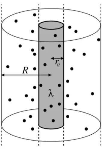
r₀ R

λ

Figure 2. Geometry of the cell model. A cylindrical rod with radiusr⁰ and line charge density λ is enclosed by a cylindrical cell of radius R. Note that within Poisson-Boltzmann theory the ions are point-like in the sense that no hard core energy term enters the free energy functionalF^PB from Eqn. (16). However, the theory does not describe individual point-ions but rather an average ionic density.

strate how the theoretical considerations presented so far can be applied to a realistic situation. We chose the cylindrical geometry since this gives us the opportunity to compare Poisson-Boltzmann theory with Manning’s sce- nario of counterion condensation. A more comprehensive and very readable introduction, also covering other geometries, is given in Ref. [18].

4.1. SPECIFICATION OF THE CELL MODEL

Consider linear polyelectrolytes of line charge density λ = e λ > ˜ 0, radius r

₀

, and length L that are distributed at a density n

_P

in a solvent characterized by a Bjerrum length ℓ

_B

. We will assume the counterions to be monovalent (z =

−

1), and at first the system does not contain additional salt. Let us enclose the polyelectrolytes by cylindrical cells of radius R and length L.

Requiring that the volume of each cell equals the volume per polyelectrolyte in the original solution gives the relation n

_P

= 1/πR

²

L, from which we derive the cell radius. If the polyelectrolytes are bent on a large scale, we will require the cell radius R to be small compared to the persistence length of the charged chains and subsequently neglect the bending. We will thus refer to the linear polyelectrolytes simply as “charged rods”.

For monovalent counterions each of these rods dissociates N

_c

= ˜ λL

of them into the solution, such that their average density is given by ¯ n

c

=

N

_c

n

_P

= ˜ λ/πR

²

. If one now neglects end-effects, i. e., if one sets L to infinity,

the problem acquires cylindrical symmetry. Observe that ¯ n

_c

is independent

of L. It is therefore a more convenient measure of the system density, since it is unaffected by the limit L

→ ∞

.

The next step is to replace the individual ion coordinates by a density n(r). The cylindrical symmetry will be exploited by assuming that this density also has cylindrical symmetry, even further, that it only depends on the radial coordinate. It is worthwhile pointing out that this statement is not a trivial assumption, for two reasons: First, just because the problem is cylindrically symmetric, the solution need not be.

²

Second, even if the average distribution only depends on the radial coordinate, there may be angular or axial fluctuations that are not taken into account if one right from the start only works with one radial coordinate.

4.2. SOLUTION OF THE POISSON-BOLTZMANN EQUATION

Employing these approximations, the Poisson-Boltzmann equation (19) in the region between r

₀

and R can be written as

y

^′′

(r) + 1

r y

^′

(r) = κ

²

e

^y(r)

. (23) Here, κ =

p

4πℓ

_B

n(R) is an inverse length (the Debye screening constant at the outer boundary) and y(r) = βeψ(r) is the dimensionless potential, which is understood to be zero at r = R. It will turn out to be convenient to introduce the dimensionless charge parameter

ξ = ˜ λℓ

_B

. (24)

It counts the number of charges along a Bjerrum length of rod and is thus a dimensionless way to measure the line charge density λ.

The boundary conditions at r = r

0

and r = R follow easily, since by Gauss’ theorem we know the value of the electric field there:

y

^′

(r

₀

) =

−

2ξ r

0

and y

^′

(R) = 0. (25)

The nonlinear boundary value problem that Eqns. (23) and (25) pose was first solved independently by Fuoss et. al [19] and Alfrey et. al [20]. It can easily be verified by insertion that the solution is given by

y(r) =

−

2 ln r

R

p

1 + γ

⁻²

cos γ ln r

R

_M

. (26)

2Broadly speaking: If a physical problem is invariant with respect to some symmetry groupS, any solution of the problem is mapped by any element ofSto another solution—

the set of solutions is closed underS. However, a particular solution need not be mapped onto itself byallelements ofS,i.e., it need not possess the full symmetry of the problem.

Let us give a simple example: The gravitational field of our sun is spherically symmetric, but the orbit of the earth is not (even if time-averaged).

The dimensionless integration constant γ is related to κ via

κ

²

R

²

= 2 (1 + γ

²

). (27)

Both γ and R

_M

are found by inserting the general solution (26) into the boundary conditions (25), which yields two coupled transcendental equa- tions:

γ ln r

0

R

_M

= arctan 1

−

ξ

γ and γ ln R

R

_M

= arctan 1

γ . (28) Subtracting them eliminates R

_M

and provides a single equation from which γ can be obtained numerically:

γ ln R

r

₀

= arctan 1

γ + arctan ξ

−

1

γ . (29)

Eqn. (29) only has a real solution for γ if ξ > ξ

_min

= ln(R/r

₀

)/(1 + ln(R/r

₀

)). For smaller charge densities γ becomes imaginary, but the solu- tion can be analytically continued by replacing γ

→

iγ and using identities like iγ tan(iγ ) =

−

γ tanh γ. However, in the following we will only be in- terested in the strongly charged case, in which the charge parameter ξ is larger than ξ

_min

.

Let us denote by φ(r) the fraction of counterions that can be found between r

₀

and r. Using n(r) = n(R) exp

{

y(r)

}

and Eqns. (26), (27), and (28), we find

φ(r) = 1 λ ˜

Z _r

r0

d¯ r 2π¯ r n(¯ r) = 1

−

1 ξ + γ

ξ tan γ ln r

R

_M

. (30)

Observe that φ(R

_M

) = 1

−

1/ξ. Hence, the second integration constant R

_M

is the distance at which the fraction 1

−

1/ξ of counterions can be found, which also implies r

₀ ≤

R

_M

< R. Due to the importance of this fraction in Manning’s theory of counterion condensation (see Sec. (4.3)), R

_M

is sometimes referred to as the “Manning radius”.

4.3. MANNING CONDENSATION

The ion distribution around a charged cylindrical rod exhibits a remark- able feature that can be unveiled by the following simple considerations [21]. Assume that the system is infinitely dilute and that there is only one counterion. In the canonical ensemble its radial distribution should be given by e

^−βH(r)

/ Tr

e

^−βH(r)

where, up to the kinetic energy and an additive

constant, the Hamiltonian is βH(r) = 2ξ ln(r/r

0

). However, the trace (per unit length) over the coordinate space is

Tr e

^−βH

=

Z ∞

r0

dr 2πr e

^{−2ξln(r/r0)}

= 2πr

²₀ Z ∞

1

dx x

^1−2ξ

, (31) which diverges for ξ < 1. Hence, the distribution function cannot be nor- malized. In other words, such rods cannot localize counterions in the limit of infinite dilution, while rods with ξ > 1 can. This led Manning to the simple idea that rods with ξ > 1 “condense” a fraction of 1

−

1/ξ of all counterions, thereby reducing (“renormalizing”) their charge parameter to an effective value of 1, while the rest of the ions remains more or less “free”, i. e., not localized [22]. This concept has subsequently been referred to as “Manning condensation” and has led to much insight into the physical chemistry of charged cylindrical macroions.

Similar arguments can be made for the infinite dilution limit in the planar and spherical case. They show that a plane always localizes all its counterions no matter how low its surface charge density is, while a sphere always loses all its counterions no matter how high its surface charge density is.

4.4. LIMITING LAWS OF THE CYLINDRICAL PB-SOLUTION

Although the PB-equation for the cylindrical geometry can be solved ana- lytically, the transcendental equation (29) for the integration constant γ has to be solved numerically. However, since for ξ > 1 its right hand side is bounded above by its zeroth and bounded below by its first order Taylor expansion, this gives an allowed interval for γ. All following considerations are restricted to the strongly charged case ξ > 1.

π

≥

γ ln R

r

₀

= arctan 1

γ + arctan ξ

−

1

γ

≥

π

−

ξ

ξ

−

1 γ (ξ > 1)

⇒

π ln

_r^R

0

≥

γ

≥

π ln

_r^R

0

+

_ξ−^ξ₁

(32)

In the limit R

→ ∞

the two bounds, and therefore γ, converge to zero. In this limit γ can be approximated by either side of inequality (32), which gives rise to various asymptotic behaviors, known as “limiting laws” for in- finite dilution. An immediate first consequence of (32) is that these asymp- totic behaviors are reached logarithmically slowly. In the following we will briefly discuss four of these limiting laws.

As we have seen above, the radius R

_M

contains the fraction 1

−

1/ξ of

ions that are condensed in the sense of Manning. The following limit shows

that R

M

scales asymptotically as the square root of the cell radius:

R

lim

→∞

R

_M

√

Rr

₀

= exp

n

ξ

−

2 2ξ

−

2

o

, (33) It can be shown [23] that a radius that is required to contain any fraction smaller than 1

−

1/ξ will remain finite in the limit R

→ ∞

, while a ra- dius containing more than this fraction will diverge asymptotically like R.

Roughly speaking, the fraction 1

−

1/ξ cannot be diluted away, which is in accordance with the localization argument given in Section 4.3.

Up to a logarithmic

³

correction the electrostatic potential is that of a rod with charge parameter 1:

R

lim

→∞

y(r) = y(r

₀

)

−

2 ln r

r

0 −

2 ln

1 + (ξ

−

1) ln r r

0

. (34) This is Manning condensation rediscovered on the level of the mean-field potential. Note, however, that the presence of the logarithmic corrections implies that the condensed ions do not sit on top of the charged rod, but rather have a radial distribution. For finite cell radii this distribution is characterized by the length R

_M

, which diverges in the dilute limit. Hence, the ions are not particularly closely confined.

The ratio between the boundary density n(R) and the average counte- rion density ¯ n

c

shows the limiting behavior

R

lim

→∞

n(R)

¯

n

_c

= lim

R→∞

1 + γ

²

2ξ = 1

2ξ . (35)

Since we have seen in Sec. 3 that the boundary density is proportional to the osmotic pressure, the ratio n(R)/¯ n

c

is equal to the ratio P/P

_id

between the actual osmotic pressure and the ideal gas pressure of a fictitious system of non-interacting particles at the same average density. This ratio is called the “osmotic coefficient”, and in the dilute limit it converges from above towards 1/2ξ < 1. The presence of the charged rod hence strongly reduces the osmotic activity of the counterions.

While Eqn. (35) implies that the boundary density goes to zero in the dilute limit, the contact density approaches a finite value:

R

lim

→∞

n(r

₀

) = 2πℓ

_B

σ ˜

²

1

−

1

ξ

2

= 2πℓ

_B

˜ σ

²

1

−

1

2πr

₀

ℓ

_B

σ ˜

2

. (36) This as well is a sign that ions must be condensed. We would like to link these two equations to the contact value theorem derived in Section 2, in

3Since the potential itself is already logarithmic, the logarithmic correction is actually of the form ln lnr.

particular to Eqn. (7). Observe that this equation is

not

satisfied. This is not a bug of the Poisson-Boltzmann approximation but rather a feature of the cylindrical geometry: The contact density is lower than in the corresponding planar case, essentially since only the fraction 1

−

1/ξ of condensed ions

“contributes” to the ion distribution function. However, in the limit r

₀ →

∞

at

fixed

surface charge density e˜ σ the charged rod becomes a charged plane, ξ = 2πℓ

_B

σr ˜

₀

diverges, and the correction factor becomes 1, such that the contact value theorem is again satisfied. Note also that ξ can be written as r

₀

/λ

_GC

, where λ

_GC

is the so called Gouy-Chapman length, the characteristic width of a planar electrical double layer forming at a surface with surface charge density e˜ σ [18]. For the contact value theorem to be valid in its planar version it is thus necessary that the characteristic extension of the charged layer is small compared to the radius of curvature of the surface—or, equivalently: ξ

≫

1. It is worth pointing out that the solution of the linearized planar Poisson-Boltzmann equation violates the contact value theorem by giving a contact density which is a factor of 2 too large.

5. Additional salt: The Donnan equilibrium

How is the Poisson-Boltzmann equation to be modified, if more than one species of ions is present? First, each ion density n

_i

(r) is assumed to be proportional to the local Boltzmann-factor, thereby generalizing Eqn. (18):

n

_i

(r) = n

_0i

e

^{−βzie ψtot(r)}

with n

_0i

= N

_i R

V

d

³

r e

^{−βzie ψtot(r)}

. (37) Second, the total charge density e

P

i

z

_i

n

_i

(r) has to satisfy Poisson’s equa- tion. This situation arises if the counterions form a mixture of different valences or if the system contains additional salt. In this section we would like to make a few remarks about the latter case.

The amount of salt can be specified by the number of salt molecules per cell. Since salt molecules are neutral (unlike counterions), their number is not restricted by the constraint of electroneutrality, and different cells may contain different numbers of salt molecules. This variation cannot be taken into account by a description focusing on just one cell and is thus neglected.

One assumes instead that the cell contains a number of salt molecules equal to the average salt concentration in the polyelectrolyte solution times the cell volume. In other words: The division of salt between the cells is assumed to be perfectly even.

If the presence of salt is due to the fact that the polyelectrolyte solution

is in contact with a salt reservoir, there is a further problem to solve: How is

the average concentration of salt molecules in the polyelectrolyte solution

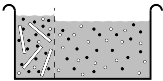
Figure 3. Solution of charged rod-like polyelectrolytes and counterions in equilibrium with a bulk salt reservoir. The membrane is permeable for everything but the macroions.

Notice that both compartments are charge neutral.

related to the concentration of salt molecules in the salt reservoir? This situation is depicted in Fig. 3 and is referred to as a “Donnan equilibrium”

[25, 26]. In the following we will address this question on the level of the cell model and Poisson-Boltzmann theory. For simplicity we will only treat the case in which all ions are monovalent.

The compartment containing the macroions will be described by a cell- model, which apart from the central rod and the counterions will contain a certain number of salt molecules, yet to be determined. Since both the counterions and the oppositely charged coions can cross the membrane, they have to be in electrochemical equilibrium. However, before we can write down a condition for that, there is an additional effect that we have to take into account: Since the charged macroions cannot leave their com- partment, their counterions also will have to remain there for reasons of electroneutrality. Hence, upon addition of salt there is a tendency for the salt to go into the other compartment, which is less “crowded”. However, this implies that in general there must be a discontinuity in the counter- and coion density across the membrane. Such a difference can only be sustained by a corresponding drop in the electrostatic potential across the membrane separating the two compartments. This potential drop is referred to as the

“Donnan potential”, Φ

_D

, and must be taken into account when balancing the electrochemical potentials.

Having said this, we can now proceed to compute electrochemical poten-

tials on both sides. On the side containing the macroions we will compute

the chemical potential at the cell boundary, where the only contribution is

the entropy term if we set the potential to zero there. In the bulk salt reser-

voir we get an entropy term corresponding to the bulk salt density, which

we call n

_b

, and a term corresponding to the Donnan potential Φ

_D

. With

n

±

being the cation and anion densities at the cell boundary, we obtain k

_B

T ln n

±

= k

_B

T ln n

_b ±

e Φ

_D

⇒

n

±

= n

_b

e

^±βeΦD

. (38) Multiplying cation and anion density gives

n

₊

n

−

= n

²_b

. (39)

That is, the bulk salt density is the geometric average of the cation and anion densities at the cell boundary. Dividing the ion densities in Eqn. (38) yields an expression for the Donnan potential:

βe Φ

_D

= 1 2 ln n

₊

n

−

(39)

= ln n

₊

n

_b

. (40)

This also shows that the Donnan potential diverges in the zero salt limit.

For sufficiently dilute solutions the osmotic pressure follows from the van’t Hoff equation βP = [solute]. Since the

excess

osmotic pressure is given by the difference between the osmotic pressures at the cell boundary acting from inside and from outside, we find

βP = n

+

+ n

−−

2n

_b ⁽³⁹⁾

=

√

n

+−√

n

−

2

≥

0. (41) Let δn

₊

= n

₊−

n

_b

denote the difference between the cation density at the outer cell boundary and the cation density in the bulk salt reservoir.

Combining Eqns. (38), (40) and (41), we can rewrite the pressure as βP

n

_b

=

√

n

₊−√

n

−

2

n

_b

=

e

^βeΦD/2−

e

^−βeΦD/22

= 4 sinh

²

1 2 ln n

₊

n

_b

= 4 sinh

²h

1 2 ln

1 + δn

₊

n

_b

i

δn+≪nb

≈

δn

+

n

_b 2

. (42)

If one wishes to determine the osmotic pressure, one has to solve the nonlinear Poisson-Boltzmann equation in the presence of salt, subject to the constraint in Eqn. (39). However, no analytical solution is known for this case. A numerical solution can be obtained in the following way: First

“guess” an initial amount of salt to be present in the cell, solve the PB equation

⁴

, compute the bulk salt concentration implied by this amount

4Two simple ways for achieving this are described in Ref. [24]. Although these authors treat the spherical case, their approach works equally well for cylindrical symmetry, since the only important point is that the problem is one-dimensional.

via Eqn. (39), adjust the salt content, and iterate until self-consistency is achieved.

An approximate treatment of the problem can be obtained from the following two assumptions:

1. If the amount of salt is small, it may not significantly disturb the counterion profile from the salt-free case. Hence, one may hope that the

counterion

concentration n

_R

at the cell boundary is still given by its value from

salt-free

Poisson-Boltzmann theory.

2. At the outer cell boundary the densities of additional cations and an- ions due to the salt are equal, say ∆n

_s

.

Given these two assumptions, the equilibrium condition (39) requires (n

R

+ ∆n

s

) ∆n

s ≈

n

²_b ⇒

2∆n

s ≈

q

n

²_R

+ (2n

_b

)

²−

n

R

. (43) Together with Eqn. (41) this gives the following approximate expression for the excess osmotic pressure:

βP

≈

n

_R

+ 2∆n

_s−

2n

_b

=

q

n

²_R

+ (2n

_b

)

²−

2n

_b

. (44) The advantage of this expression is that it requires only the knowledge of the counterion density n

_R

at the outer cell boundary from salt-free Poisson- Boltzmann theory, which is much easier to determine than the solution including the salt explicitly.

⁵

The above approximation is good if the counterion concentration is large compared to the salt concentration. In the opposite limit of excess salt concentration Eqn. (44) behaves asymptotically like

βP n

_b

= 2

r

1 + n

_R

2n

_b

2

−

1

≈

2

1 + 1 2

n

_R

2n

_b

2

−

1

= n

_R

2n

_b

2

. (45) Since n

R

is given by ¯ n

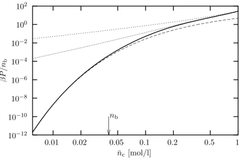
c

times the osmotic coefficient, which does not strongly vary with density, this equation implies that in the salt dominated case the osmotic pressure varies quadratically with the average counterion concentration. However, this is not born out by a numerical solution of the Poisson-Boltzmann equation with added salt, which shows an exponential behavior (see Fig. 4). The latter can be understood by the following simple argument: For large salt content the counterion and coion density profiles can be expected to merge exponentially with a bulk Debye-H¨ uckel screening constant κ

_D

=

√

8πℓ

_B

n

_b

. We may thus assume that

δn

₊ ∝

n

_b

e

^−κDR

. (46)

5It requires only the numerical solution of the transcendental equation (29), not the numerical solution of a nonlinear differential equation.

n

_b

¯

n

c

[mol/l]

βP/nb

1 0.5 0.2

0.1 0.05

0.02 0.01

10

²

10

⁰

10

⁻²

10

⁻⁴

10

⁻⁶

10

⁻⁸

10

⁻¹⁰

10

⁻¹²

Figure 4. Ionic contribution to the osmotic pressureβP of a DNA solution divided by bulk salt concentrationn^b as a function of average counterion concentration

¯

n^c. The bulk salt concentration isn^b= 40 mmol/l. The solid line is the prediction of the Poisson-Boltzmann equation (taking into account counterions and salt), the (upper) fine dashed line is from Poisson-Boltzmann theory without salt. The short dashed line is the approximation from Eqn. (44) and the long dashed line is a fit to Eqn. (48) within the range ¯n^c= 6−10 mmol/l.

Since the cell radius is related to the average counterion concentration via

¯

n

_c

= ˜ λ/πR

²

, we can write together with Eqn. (42) βP

n

_b ∝

exp

{−

2κ

_D

R

}

= exp

n

−

2

p

8πℓ

_B

n

_b

q

λ/π ˜ n ¯

_co

. (47)

Taking the logarithm we finally see log

βP n

_b

= C

₁−

C

₂ r

n

_b

¯

n

_c

(48)

with some constants C

₁

and C

₂

.

This functional dependence should hold whenever n

_b

/¯ n

_c≫

1. However,

it also demonstrates that the range of validity of the cell model reaches its

limit for high salt concentrations. As increasingly more salt is added to the

system the osmotic pressure of the ions vanishes exponentially. However,

this does not imply that the total osmotic pressure of the polyelectrolyte

solution vanishes, since we have neglected the contribution coming from the

macroions [27]. Since the latter generally depends on observables which are largely irrelevant for the cell model (e. g., the degree of polymerization), this model must break down here.

6. Outlook

We presented in our brief introduction two of the most common approxima- tions encountered in the theory of charged macromolecules: The cell-model and Poisson-Boltzmann theory. Where can one go from here?

One of the key deficiencies of Poisson-Boltzmann theory is the neglect of interparticle correlations. We have seen how this arose from the assump- tion of a product state, which subsequently led to a simple (local) density functional theory. An important theorem originally due to Hohenberg and Kohn states that there actually

exists

a density functional which gives the correct free energy of the full system and which differs from the Poisson- Boltzmann functional by an additional term that takes into account the ef- fects of correlations.

⁶

Although the theorem does not specify what this func- tional looks like, it shows that attempts that go beyond Poisson-Boltzmann theory but stay on a density functional level are not futile. Indeed, various local [29] and nonlocal [30] corrections to the Poisson-Boltzmann functional have been suggested in the past.

The Coulomb problem has been treated in a field-theoretic way, i. e., the classical partition function is transformed via a Hubbard-Stratonovich transformation into a functional integral [31]. Poisson-Boltzmann theory is rediscovered as the saddle-point of this field theory, and higher order cor- rections can in principle be obtained using the large and well-established toolbox of field-theoretic perturbation theory. There also exists the possibil- ity to approximate the functional integral in the limit opposite to Poisson- Boltzmann theory, when correlations dominate the system [32]. All this is thoroughly discussed in the lecture notes by Moreira and Netz [17].

A different route to incorporate correlations is offered by integral equa- tion theories. Their key idea is to first derive exact equations for various correlation functions and then introduce some approximate relations be- tween them, based for instance on perturbation expansions, which lead to integral equations that implicitly give the desired correlation functions.

This approach and its relation to Poisson-Boltzmann and Debye-H¨ uckel theory is the topic of the lecture of Kjellander [6].

A further method for dealing with correlations is to simulate the systems on a computer and explicitly keep track of all the ions—or even solvent molecules. This approach has become an increasingly important tool for both describing real systems as well as testing approximate theories. More

6A good introduction into this topic can be found in Ref. [28].

details can be found in the lectures of J¨ onsson and Wennerstr¨ om [3] and Holm and Kremer [33].

Going beyond the cell model and taking the actual shape of polyelec- trolytes into account is in general an extremely difficult business. However, a remarkable amount of information can be obtained by using some (or, better yet, a lot of) physical insight and writing the free energy as a sum of a few terms which account for the most relevant physical properties of the system (for instance the chain elasticity, electrostatic self-energy or hydrophobic interactions) and possibly some variational parameters. Since in doing so all prefactors are neglected (it only matters how one observ- able “scales” with another) these approaches are known as scaling theories.

Joanny gives an introduction and a few famous applications in his lecture [34].

All these approaches reach beyond the cell-model and/or the Poisson- Boltzmann equation. They boldly go where no mean-field theory has gone before. However, we believe that in order to appreciate their efforts it is worthwhile to know where they came from. It was the intention of this chapter to provide some of that knowledge.

Acknowledgments

M. D. would like to thank P. L. Hansen and I. Borukhov for stimulating discussions.

References

1. C. Holm, P. K´ekicheff, and R. Podgornik, eds.Electrostatic Effects in Soft Matter and Biophysics, Proceedings of the Les Houches NATO-ASI, Oct. 1-13, 2000, NATO Science Series II - Mathematics, Physics and Chemistry, Vol. 46, Kluwer, Dordrecht (2001).

2. A. Katchalsky, Pure Appl. Chem.26, 327 (1971).

3. B. J¨onnson and H. Wennerstr¨om, contribution in Ref. 1.

4. P. Debye and E. H¨uckel, Phys. Z.24, 185 (1923).

5. T. L. Hill,An Introduction to Statistical Thermodynamics, Dover Publications, New York (1986). D. A. McQuarrie, Statistical Mechanics, Harper Collins, New York (1976).

6. R. Kjellander, contribution in Ref. 1.

7. F. H. Stillinger Jr. and R. Lovett, J. Chem. Phys.48, 3858 (1968); F. H. Stillinger Jr. and R. Lovett, J. Chem. Phys.49, 1991 (1968).

8. S. L. Carnie and D. Y. C. Chan, Chem. Phys. Lett.77, 437 (1981).

9. D. Henderson and L. Blum, J. Chem. Phys.69, 5441 (1978).

10. D. Henderson, L. Blum, and J. L. Lebowitz, J. Electroanal. Chem.102, 315 (1979).

11. H. Wennerstr¨om, B. J¨onsson, and P. Linse, J. Chem. Phys.76, 4665 (1982).

12. L. D. Landau and E. M. Lifshitz,The classical Theory of Fields, Addison-Wesley, Cambridge (Mass.) (1951).

13. D. C. Grahame, Chem. Rev.41, 441 (1947).