Introduction to Nonlinear Regression

(1)

Introduction to Nonlinear Regression

Andreas Ruckstuhl

IDP Institut für Datenanalyse und Prozessdesign ZHAW Zürcher Hochschule für Angewandte Wissenschaften

October 2010

^∗†

1. The Nonlinear Regression Model

a The Regression Model. Regression studies the relationship between a variable of interest Y and one or moreexplanatory or predictor variables x^(j). The general model is

Y_i=hhx⁽¹⁾_i , x⁽²⁾_i , . . . , x^(m)_i ; θ₁, θ₂, . . . , θ_pi+E_i.

Here, h is an appropriate function that depends on the explanatory variables and parameters, that we want to summarize with vectors x = [x⁽¹⁾_i , x⁽²⁾_i , . . . , x^(m)_i ]^T and θ = [θ1, θ2, . . . , θp]^T. The unstructured deviations from the function h are described via the random errors E_i. The normal distribution is assumed for the distribution of this random error, so

E_i∼ N^D0, σ²^E , independent.

b The Linear Regression Model. In (multiple) linear regression, functions h are considered that are linear in the parameters θ_j,

hhx⁽¹⁾_i , x⁽²⁾_i , . . . , x^(m)_i ; θ₁, θ₂, . . . , θ_pi=θ₁x_e⁽¹⁾_i +θ₂x_e⁽²⁾_i +. . .+θ_px_e^(p)_i ,

where the x_e^(j) can be arbitrary functions of the original explanatory variables x^(j). (Here the parameters are usually denoted as β_j instead of θ_j.)

c The Nonlinear Regression ModelIn nonlinear regression, functions h are considered that can not be written as linear in the parameters. Often such a function is derived from theory. In principle, there are unlimited possibilities for describing the determin- istic part of the model. As we will see, this flexibility often means a greater effort to make statistical statements.

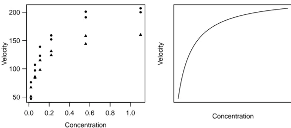
Example d Puromycin. The speed with which an enzymatic reaction occurs depends on the concentration of a substrate. According to the information from Bates and Watts (1988), it was examined how a treatment of the enzyme with an additional substance called Puromycin influences this reaction speed. The initial speed of the reaction is chosen as the variable of interest, which is measured via radioactivity. (The unit of the variable of interest is count/min²; the number of registrations on a Geiger counter per time period measures the quantity of the substance present, and the reaction speed is proportional to the change per time unit.)

(3)

2 1. The Nonlinear Regression Model

0.0 0.2 0.4 0.6 0.8 1.0 50

100 150 200

Concentration

Velocity

Concentration

Velocity

Figure 1.d:Puromycin Example. (a) Data (• treated enzyme; △ untreated enzyme) and (b) typical course of the regression function.

The relationship of the variable of interest with the substrate concentration x (in ppm) is described via the Michaelis-Menten function

hhx;θi= θ₁x θ₂+x .

An infinitely large substrate concentration (x→ ∞) results in the ”asymptotic” speed θ₁. It has been suggested that this variable is influenced by the addition of Puromycin.

The experiment is therefore carried out once with the enzyme treated with Puromycin and once with the untreated enzyme. Figure 1.d shows the result. In this section the data of the treated enzyme is used.

Example e Oxygen Consumption. To determine the biochemical oxygen consumption, river water samples were enriched with dissolved organic nutrients, with inorganic materials, and with dissolved oxygen, and were bottled in different bottles. (Marske, 1967, see Bates and Watts (1988)). Each bottle was then inoculated with a mixed culture of microor- ganisms and then sealed in a climate chamber with constant temperature. The bottles were periodically opened and their dissolved oxygen content was analyzed. From this the biochemical oxygen consumption [mg/l] was calculated. The model used to con- nect the cumulative biochemical oxygen consumption Y with the incubation timex, is based on exponential growth decay, which leads to

hhx, θi=θ₁1−e^−θ²^x

. Figure 1.e shows the data and the regression function to be applied.

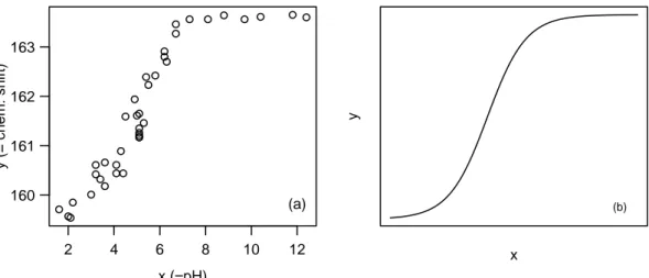
Example f From Membrane Separation Technology (Rapold-Nydegger (1994)). The ratio of protonated to deprotonated carboxyl groups in the pores of cellulose membranes is dependent on the pH value x of the outer solution. The protonation of the carboxyl carbon atoms can be captured with ¹³C-NMR. We assume that the relationship can be written with the extended “Henderson-Hasselbach Equation” for polyelectrolytes

log₁₀

θ₁−y y−θ₂

=θ₃+θ₄x ,

(4)

1. The Nonlinear Regression Model 3

1 2 3 4 5 6 7

8 10 12 14 16 18 20

Days

Oxygen Demand

Days

Oxygen Demand

Figure 1.e:Oxygen consumption example. (a) Data and (b) typical shape of the regression function.

2 4 6 8 10 12

160 161 162 163

x (=pH)

y (= chem. shift)

(a)

x

y

(b)

Figure 1.f:Membrane Separation Technology.(a) Data and (b) a typical shape of the regression function.

where the unknown parameters are θ₁, θ₂ and θ₃ >0 and θ₄<0. Solving for y leads to the model

Y_i =hhxi;θi+E_i= θ₁+θ₂10^θ³^+θ⁴^xⁱ 1 + 10^θ³^+θ⁴^xⁱ +E_i.

The regression funtion hhx_i, θi for a reasonably chosen θ is shown in Figure 1.f next to the data.

g A Few Further Examples of Nonlinear Regression Functions:

• Hill Model (Enzyme Kinetics): hhxi, θi=θ₁x^θ_i³/(θ₂+x^θ_i³)

For θ₃ = 1 this is also known as the Michaelis-Menten Model (1.d).

• Mitscherlich Function (Growth Analysis): hhxi, θi=θ₁+θ₂exphθ3x_ii.

• From kinetics (chemistry) we get the function

hhx⁽¹⁾_i , x⁽²⁾_i ;θi= exph−θ₁x⁽¹⁾_i exph−θ₂/x⁽²⁾_i ii.

(5)

4 1. The Nonlinear Regression Model

• Cobbs-Douglas Production Function

h^Dx⁽¹⁾_i , x⁽²⁾_i ;θ^E =θ₁ x⁽¹⁾_i ^θ² x⁽²⁾_i ^θ³.

Since useful regression functions are often derived from the theory of the application area in question, a general overview of nonlinear regression functions is of limited benefit. A compilation of functions from publications can be found in Appendix 7 of Bates and Watts (1988).

h Linearizable Regression Functions. Some nonlinear regression functions can be lin- earized through transformation of the variable of interest and the explanatory variables.

For example, a power function

hhx;θi=θ₁x^θ²

can be transformed for a linear (in the parameters) function lnhhhx;θii= lnhθ1i+θ2lnhxi=β0+β1x ,e

whereβ₀ = lnhθ1i, β₁ = θ₂ and x_e= lnhxi. We call the regression function h lin- earizable, if we can transform it into a function linear in the (unknown) parameters via transformations of the arguments and a monotone transformation of the result.

Here are some more linearizable functions (also see Daniel and Wood, 1980):

hhx, θi= 1/(θ1+θ2exph−xi) ←→ 1/hhx, θi=θ1+θ2exph−xi hhx, θi=θ1x/(θ2+x) ←→ 1/hhx, θi= 1/θ1+θ2/θ11

x

hhx, θi=θ1x^θ² ←→ lnhhhx, θii= lnhθ1i+θ2lnhxi hhx, θi=θ1exphθ2ghxii ←→ lnhhhx, θii= lnhθ1i+θ2ghxi

hhx, θi= exph−θ1x⁽¹⁾exph−θ2/x⁽²⁾ii ←→ lnhlnhhhx, θiii= lnh−θ1i+ lnhx⁽¹⁾i −θ2/x⁽²⁾ hhx, θi=θ1 x⁽¹⁾^θ²

x⁽²⁾^θ³

←→ lnhhhx, θii= lnhθ1i+θ2 lnhx⁽¹⁾i+θ3 lnhx⁽²⁾i.

The last one is the Cobbs-Douglas Model from 1.g.

i The Statistically Complete Model. A linear regression with the linearized regression function in the referred-to example is based on the model

lnhYii=β₀+β₁x_e_i+E_i ,

where the random errors E_i all have the same normal distribution. We back transform this model and thus get

Yi =θ1·x^θ² ·E^ei

with E^e_i = exphEii. The errors E^e_i, i= 1, . . . , n now contribute multiplicatively and are lognormal distributed! The assumptions about the random deviations are thus now drastically different than for a model that is based directily on h,

Y_i =θ₁·x^θ²+E_i^∗

with random deviations E^∗_i that, as usual, contribute additively and have a specific normal distribution.

(6)

2. Methodology for Parameter Estimation 5

A linearization of the regression function is therefore advisable only if the assumptions about the random deviations can be better satisfied - in our example, if the errors actually act multiplicatively rather than additively and are lognormal rather than normally distributed. These assumptions must be checked with residual analysis.

j *Note: In linear regression it has been shown that the variance can be stabilized with certain transformations (e.g. logh·i,√

·). If this is not possible, in certain circumstances one can also perform a weighted linear regression . The process is analogous in nonlinear regression.

k The introductory examples so far:

We have spoken almost exclusively of regression functions that only depend on one original variable. This was primarily because it was possible to fully illustrate the model graphically. The ensuing theory also functions well for regression functions hhx;θi, that depend on several explanatory variables x= [x⁽¹⁾, x⁽²⁾, . . . , x^(m)].

2. Methodology for Parameter Estimation

a The Principle of Least Squares. To get estimates for the parameters θ= [θ₁,θ₂, . . ., θ_p]^T, one applies, like in linear regression calculations, the principle of least squares.

The sum of the squared deviations S(θ) :=

Xn i=1

(y_i−η_ihθi)² mit η_ihθi:=hhxi;θi

should thus be minimized. The notation where hhxi;θi is replaced by η_ihθi is reasonable because [xi, yi] is given by the measurement or observation of the data and only the parameters θ remain to be determined.

Unfortunately, the minimum of the squared sum and thus the estimation can not be given explicitly as in linear regression. Iterative numeric procedureshelp further.

The basic ideas behind the common algorithm will be sketched out here. They also form the basis for the easiest way to derive tests and confidence intervals.

b Geometric Illustration. The observed values Y = [Y₁, Y₂, . . . , Y_n]^T determine a point in n-dimensional space. The same holds for the ”model values” ηhθi = [η1hθi, η2hθi, . . . , ηnhθi]^T for given θ.

Take note! The usual geometric representation of data that is standard in, for example, multivariate statistics, considers the observations that are given by m variables x^(j), j = 1,2, . . . , m,as points in m-dimensional space. Here, though, we consider the Y- and η-values of all n observations as points in n-dimensional space.

Unfortunately our idea stops with three dimensions, and thus with three observations.

So, we try it for a situation limited in this way, first for simple linear regression.

As stated, the observed values Y = [Y₁, Y₂, Y₃]^T determine a point in 3-dimensional space. For given parameters β₀ = 5 and β₁ = 1 we can calculate the model values η_i^Dβ^E=β₀+β₁x_i and represent the corresponding vectorη^Dβ^E=β₀1+β₁x as a point.

We now ask where all points lie that can be achieved by variation of the parameters.

These are the possible linear combinations of the two vectors 1 andxand thus form the

(7)

6 2. Methodology for Parameter Estimation

plane ”spanned by 1 and x” . In estimating the parameters according to the principle of least squares, geometrically represented, the squared distance between Y and η^Dβ^E is minimized. So, we want the point on the plane that has the least distance to Y. This is also called the projection of Y onto the plane. The parameter values that correspond to this point η_bare therefore the estimated parameter values β^b= [β^b₀,β^b₁]^T. Now a nonlinear function, e.g. hhx;θi = θ₁exph1−θ₂xi, should be fitted on the same three observations. We can again ask ourselves where all points ηhθi lie that can be achieved through variations of the parameters θ₁ and θ₂. They lie on a two-dimensional curved surface (called themodel surface in the following) in three- dimensional space. The estimation problem again consists of finding the point η_b on the model surface that lies nearest to Y. The parameter values that correspond to this point η_b, are then the estimated parameter values θ^b= [θ^b₁,θ^b₂]^T.

c Solution Approach for the Minimization Problem. The main idea of the usual algorithm for minimizing the sum of squared deviations (see 2.a) goes as follows: If a preliminary best value θ^(ℓ) exists, we approximate the model surface with the plane that touches the surface at the point η^Dθ^(ℓ)^E=h^Dx;θ^(ℓ)^E. Now we seek the point in this plane that lies closest to Y. This amounts to the estimation in a linear regression problem. This new point lies on the plane, but not on the surface, that corresponds to the nonlinear problem. However, it determines a parameter vector θ^(ℓ+1) and with this we go into the next round of iteration.

d Linear Approximation. To determine the approximated plane, we need the partial derivative

A^(j)_i hθi:= ∂η_ihθi

∂θ_j ,

which we can summarize with a n×p matrix A. The approximation of the model surface ηhθi by the ”tangential plane” in a parameter value θ^∗ is

η_ihθi ≈η_ihθ^∗i+A⁽¹⁾_i hθ^∗i(θ₁−θ₁^∗) +...+A^(p)_i hθ^∗i(θ_p−θ_p^∗) or, in matrix notation,

ηhθi ≈ηhθ^∗i+Ahθ^∗i(θ−θ^∗).

If we now add back in the random error, we get a linear regression model Ye = Ahθ^∗iβ+E

with the ”preliminary residuals” Y^e_i =Y_i−η_ihθ^∗i as variable of interest, the columns of A as regressors and the coefficients β_j =θ_j−θ_j^∗ (a model without intercept β₀).

(8)

2. Methodology for Parameter Estimation 7

e Gauss-Newton Algorithm. The Gauss-Newton algorithm consists of, beginning with a start valueθ⁽⁰⁾ forθ, solving the just introduced linear regression problem forθ^∗=θ⁽⁰⁾ to find a correction β and from this get an improved value θ⁽¹⁾ =θ⁽⁰⁾+β. For this, again, the approximated model is calculated, and thus the ”preliminary residuals”

Y −η^Dθ⁽¹⁾^E and the partial derivatives A^Dθ⁽¹⁾^E are determined, and this gives us θ₂. This iteration step is continued as long as the correction β is negligible. (Further details can be found in Appendix A.)

It can not be guaranteed that this procedure actually finds the minimum of the squared sum. The chances are better, the better the p-dimensionale model surface at the minimum θ^b= (θ^b₁, . . . ,θ^b_p)^T can be locally approximated by a p-dimensional ”plane”

and the closer the start value θ⁽⁰⁾ is to the solution being sought.

*Algorithms comfortably determine the derivative matrix A numerically. In more complex problems the numerical approximation can be insufficient and cause convergence problems. It is then advantageous if expressions for the partial derivatives can be arrived at analytically. With these the derivative matrix can be reliably numerically determined and the procedure is more likely to converge (see also Chapter 6).

f Initial Values. A iterative procedure requires a starting value in order for it to be applied at all. Good starting values help the iterative procedure to find a solution more quickly and surely. Some possibilities to get these more or less easily are here briefly presented.

g Initial Value from Prior Knowledge. As already noted in the introduction, nonlinear models are often based on theoretical considerations from the application area in question. Already existing prior knowledge from similar experiments can be used to get an initial value. To be sure that the chosen start value fits, it is advisable to graphically represent the regression function hhx;θi for various possible starting values θ=θ⁰ together with the data (e.g., as in Figure 2.h, right).

h Start Values via Linearizable Regression Functions. Often, because of the distribution of the error, one is forced to remain with the nonlinear form in models with linearizable regression functions. However, the linearized model can deliver starting values.

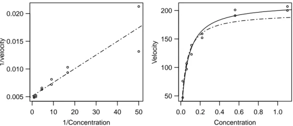
In the Puromycin Example the regression function is linearizable: The reciprocal values of the two variables fulfill

e y= 1

y ≈ 1

hhx;θi = 1 θ₁ +θ₂

θ₁ 1

x =β₀+β₁x ._e

The least squares solution for this modified problem isβ^b= [β^b₀,β^b₁]^T = (0.00511, 0.000247)^T (Figure 2.h (a)). This gives the initial value

θ⁽⁰⁾₁ = 1/β^b₀= 196, θ₂⁽⁰⁾=β^b₁/β^b₀ = 0.048.

(9)

8 3. Approximate Tests and Confidence Intervals

0 10 20 30 40 50

0.005 0.010 0.015 0.020

1/Concentration

1/velocity

0.0 0.2 0.4 0.6 0.8 1.0 50

100 150 200

Concentration

Velocity

Figure 2.h:Puromycin Example. Left: Regression line in the linearized problem. Right: Re- gression function hhx;θi for the initial values θ = θ⁽⁰⁾ ( ) and for the least squares estimation θ=θb(——–).

i Initial Values via Geometric Meaning of the Parameter. It is often helpful to consider the geometrical features of the regression function.

In the Puromycin Example we can thus arrive at an initial value in another, in- structive way: θ₁ is the y value for x=∞. Since the regression function is monotone increasing, we can use the maximal yi-value or a visually determined ”asymptotic value” θ⁰₁ = 207 as initial value for θ₁. The parameter θ₂ is the x-value, at which y reaches half of the asymptotic value θ₁. This gives θ⁰₂ = 0.06.

The initial values thus result from the geometrical meaning of the parameters and a coarse determination of the corresponding aspects of a curve ”fitted by eye.”

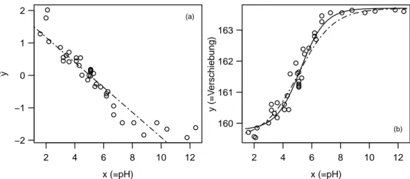
Example j Membrane Separation Technology.In the Membrane Separation example we let x →

∞, so hhx;θi → θ₁ (since θ₄ <0); for x → −∞, hhx;θi → θ₂. From Figure 1.f(a) along with the data shows θ₁ ≈163.7 and θ₂≈159.5. We know θ₁ and θ₂, so we can linearize the regression function through

e

y:= log₁₀hθ⁽⁰⁾₁ −y

y−θ₂⁽⁰⁾i=θ₃+θ₄x .

We speak of a conditional linearizable function. The linear regression leads to the initial value θ⁽⁰⁾₃ = 1.83 and θ₄⁽⁰⁾=−0.36.

With this initial value the algorithm converges to the solution θ^b1 = 163.7, θ^b2 = 159.8, θb₃ = 2.675 and θ^b₄ =−0.512. The functions hh·;θ⁽⁰⁾i and hh·;θi^b are shown in Figure 2.j(b).

*The property of conditional linearity of a function can also be useful for developing an algorithm specially suited for this situation (see e.g. Bates and Watts, 1988).

3. Approximate Tests and Confidence Intervals

a The estimator θ^b gives the value of θ that fits the data optimally. We now ask which parameter values θ are compatible with the observations. The confidence region is

(10)

3. Approximate Tests and Confidence Intervals 9

2 4 6 8 10 12

−2

−1 0 1 2

x (=pH)

y

(a)

2 4 6 8 10 12

160 161 162 163

x (=pH)

y (=Verschiebung)

(b)

Figure 2.j:Membrane Separation Technology Example. (a) Regression line, which is used for determining the initial values for θ3 and θ4. (b) Regression function hhx;θi for the initial value θ=θ⁽⁰⁾ ( ) and for the least squares estimation θ=θb(——–).

the set of all these values. For an individual parameter θ_j the confidence region is the confidence interval.

The results that now follow are based on the fact that the estimatorθ^bis asymptotically multivariate normally distributed. For an individual parameter that leads to a “z-Test”

and the corresponding confidence interval; for several parameters the corresponding Chi-Square test works and gives elliptical confidence regions.

b The asymptotic propertiesof the estimator can be derived from the linear approximation. The problem of nonlinear regression is indeed approximately equal to the linear regression problem mentioned in 2.d

Ye = Ahθ^∗iβ+E ,

if the parameter vectorθ^∗, which is used for the linearization lies near to the solution. If the estimation procedure has converged (i.e. θ^∗=θ), then^b β = 0 – otherwise this would not be the solution. The standard error of the coefficients β – and more generally the covariance matrix of β^b – then correspond approximately to the corresponding values for θ^b.

*A bit more precisely: The standard errors characterize the uncertainties that are generated by the random fluctuations in the data. The available data have led to the estimation value bθ. If the data were somewhat different, then bθ would still be approximately correct, thus we accept that it is good enough for the linearization. The estimation of β for the new data set would thus lie as far from the estimated value for the available data, as this corresponds to the distribution of the parameter in the linearized problem.

c Asymptotic Distribution of the Least Squares Estimator. From these considerations it follows: Asymptotically the least squares estimator θ^b is normally distributed (and consistent) and therefore

θb∼ N^a

θ,V hθi n

,

with asymptotic covariance matrix V hθi =σ²(Ahθi^T Ahθi)⁻¹, where Ahθi is the n×p matrix of the partial derivatives (see 2.d).

(11)

To determine the covariance matrix Vhθi explicitly, Ahθi is calculated at the point θb instead of the unknown point θ, and for the error variance σ² the usual estimator is plugged

d V hθi=σ_b²

A^Dθb^E^T A^Dθb^E

−1

mit σ_b² = Shθi^b

n−p = 1 n−p

Xn i=1

y_i−η_i^Dθ^b^E².

With this the distribution of the estimated parameters is approximately determined, from which, like in linear regression, standard error and confidence intervals can be derived, or confidence ellipses (or ellipsoids) if several variables are considered at once.

The denominator n−p in σ_b² is introduced in linear regression to make the estimator unbiased. – Tests and confidence intervals are not determined with the normal and chi-square distribution, but with the t and F distributions. There it is taken into account that the estimation of σ² causes an additional random fluctuation. Even if the distribution is no longer exact, the approximations get more exact if we do this in nonlinear regression. Asymptotically the difference goes to zero.

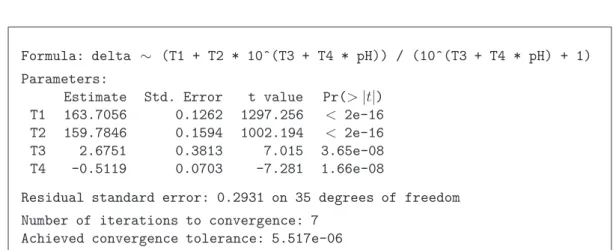
Example d Membrane Separation Technology. A computer output for the Membrane Separa- tion example shows Table 3.d. The estimations of the parameters are in the column

”Value”, followed by the estimated approximate standard error and the test statistics (”t value”), that are approximately t_n−p distributed. In the last row the estimated standard deviation σ_b of the random error E_i is given.

From this output, in linear regression the confidence intervals for the parameters can be determined: The approximate 95% confidence interval for the parameter θ₁ is

163.706±q_0.975^t³⁵ ·0.1262 = 163.706±0.256 .

Formula: delta ∼ (T1 + T2 * 10ˆ(T3 + T4 * pH)) / (10ˆ(T3 + T4 * pH) + 1) Parameters:

Estimate Std. Error t value Pr(>|t|) T1 163.7056 0.1262 1297.256 < 2e-16 T2 159.7846 0.1594 1002.194 < 2e-16 T3 2.6751 0.3813 7.015 3.65e-08 T4 -0.5119 0.0703 -7.281 1.66e-08

Residual standard error: 0.2931 on 35 degrees of freedom Number of iterations to convergence: 7

Achieved convergence tolerance: 5.517e-06

Table 3.d:Membrane Separation Technology Example: Rsummary of the fitting.

(12)

3. Approximate Tests and Confidence Intervals 11

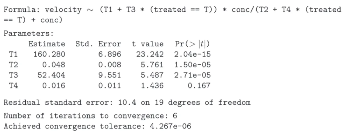
Example e Puromycin. For checking the influence of treating an enzyme with Puromycin of the postulated form (1.d) a general model for the data with and without the treatment can be formulated as follows:

Y_i= (θ₁+θ₃z_i)x_i

θ₂+θ₄z_i+x_i +E_i .

Where z is the indicator variable for the treatment (z_i= 1, if treated, otherwise =0).

Table 3.e shows that the parameterθ4 at the 5% level is not significantly different from 0, since the P value of 0.167 is larger then the level (5%). However, the treatment has a clear influence, which is expressed through θ₃; the 95% confidence interval covers the region 52.398±9.5513·2.09 = [32.4,72.4] (the value 2.09 corresponds to the 0.975 quantile of the t₁₉ distribution).

Formula: velocity ∼ (T1 + T3 * (treated == T)) * conc/(T2 + T4 * (treated

== T) + conc) Parameters:

Estimate Std. Error t value Pr(>|t|) T1 160.280 6.896 23.242 2.04e-15 T2 0.048 0.008 5.761 1.50e-05 T3 52.404 9.551 5.487 2.71e-05

T4 0.016 0.011 1.436 0.167

Residual standard error: 10.4 on 19 degrees of freedom Number of iterations to convergence: 6

Achieved convergence tolerance: 4.267e-06

Table 3.e:Rsummary of the fit for the Puromycin example.

f Confidence Intervals for Function Values. Besides the parameters, the function value hhx0, θi for a given x₀ is of interest. In linear regression the function value h^Dx₀, β^E= x^T₀β =:η₀ is estimated by η_b₀ =x^T₀β^b and the estimated (1−α) confidence interval for it is

b

η₀±q^t_1−α/2^n−p ·sehη_b₀i with sehη_b₀i=σ_b q

x^T_o(X^TX)⁻¹x_o .

With analogous considerations and asymptotic approximation we can specify confidence intervals for the function values hhx0;θi for nonlinear h. If the function η₀^Dθ^b^E:=h^Dx₀,θ^b^E is approximated at the point θ, we get

η_ohθi ≈^b η_ohθi+a^T_o (θ^b−θ) mit a_o= ∂hhxo, θi

∂θ .

(If x₀ is equal to an observed x_i, then a₀ equals the corresponding row of the matrix A from 2.d.) The confidence interval for the function value η₀hθi:=hhx0, θi is then approximately

η₀^Dθ^bÊ±q^t_1−α/2^n−p ·se^Dη₀^Dθ^bÊE mit se^Dη₀^Dθ^bÊE=σ_b r

ab_o^TA^Dθb^E^T A^Dθb^E⁻¹a_b_o. In this formula, again the unknown values are replaced by their estimations.

(13)

1.0 1.2 1.4 1.6 1.8 2.0 2.2 0

1 2 3

Years^(1/3)

log(PCB Concentration)

0 2 4 6 8

0 5 10 15 20 25 30

Days

Oxygen Demand

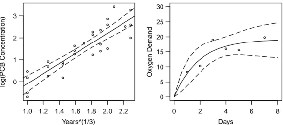
Figure 3.g:Left: Confidence band for an estimated line for a linear problem. Right: Confidence band for the estimated curve hhx, θi in the oxygen consumption example.

g Confidence Band. The expression for the (1−α) confidence interval for ηohθi :=

hhx_o, θi also holds for arbitrary x_o. As in linear regression, it is obvious to represent the limits of these intervals as a ”confidence band” that is a function of x_o, as this Figure 3.g shows for the two examples of Puromycin and oxygen consumption.

Confidence bands for linear and nonlinear regression functions behave differently: For linear functions this confidence band is thinnest by the center of gravity of the explanatory variables and gets gradually wider as it move out (see Figure 3.g, left). In the nonlinear case, the bands can be arbitrary. Because the functions in the “Puromycin”

and “Oxygen Consumption’ must go through zero, the interval shrinks to a point there.

Both models have a horizontal asymptote and therefore the band reaches a constant width for large x (see Figure 3.g, right) .

h Prediction Interval. The considered confidence band indicates where theideal func- tion values hhxi, and thus the expected values of Y for givenx, lie. The question, in which region future observations Y₀ for given x₀ will lie, is not answered by this.

However, this is often more interesting than the question of the ideal function value;

for example, we would like to know in which region the measured value of oxygen consumption would lie for an incubation time of 6 days.

Such a statement is a prediction about arandom variableand is different in principle from a confidence interval, which says something about aparameter, which is a fixed but unknown number. Corresponding to the question posed, we call the region we are now seeking a prediction interval or prognosis interval. More about this in Chapter 7.

i Variable Selection. In nonlinear regression, unlike linear regression, variable selection is not an important topic, because

• a variable does not correspond to each parameter, so usually the number of parameters is different than the number of variables,

• there are seldom problems where we need to clarify whether an explanatory variable is necessary or not – the model is derived from the subject theory.

However, there is sometimes a reasonable question of whether a portion of the parame-

(14)

4. More Precise Tests and Confidence Intervals 13

ters in the nonlinear regression model can appropriately describe the data (see Beispiel Puromycin).

4. More Precise Tests and Confidence Intervals

a The quality of the approximate confidence region depends strongly on the quality of the linear approximation. Also the convergence properties of the optimization algorithms are influenced by the quality of the linear approximation. With a somewhat larger computational effort, the linearity can be checked graphically and, at the same time, we get a more precise confidence interval.

b F Test for Model Comparison. To test a null hypothesis θ = θ^∗ for the whole parameter vector or also θ_j =θ^∗_j for an individual component, we can use an F-Test for model comparisonlike in linear regression. Here, we compare the sum of squares Shθ^∗i that arises under the null hypothesis with the sum of squares Shθi. (For^b n→ ∞ the F test is the same as the so-called Likelihood Quotient test, and the sum of squares is, up to a constant, equal to the log likelihood.)

Now we consider the null hypothesis θ=θ^∗ for the whole parameter vector. The test statistic is

T = n−p p

Shθ^∗i −Shθi^b Shθi^b

∼a F_p,n−p . From this we get a confidence region

nθ Shθi ≤Shθi^b 1 +_n−p^p q^o

where q =q_1−α^F^p,n−p is the (1−α) quantile of the F distribution with p and n−p degrees of freedom.

In linear regression we get the same exact confidence region if we use the (multivariate) normal distribution of the estimator β^b. In the nonlinear case the results are different.

The region that is based on the F tests is not based on the linear approximation in 2.d and is thus (much) more exact.

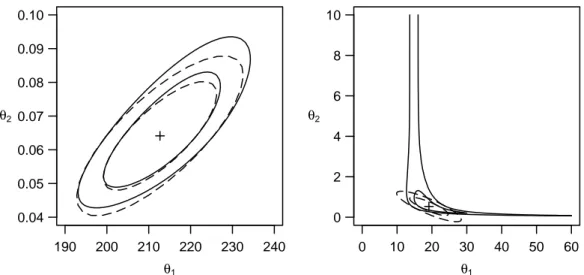
c Exact Confidence Regions for p=2. If p= 2, we can find the exact confidence region by calculating Shθi on a grid of θ values and determine the borders of the region through interpolation, as is familiar for contour plots. In Figure 4.c are given the contours together with the elliptical regions that result from linear approximation for the Puromycin example (left) and theoxygen consumption example (right).

For p > 2 contour plots do not exist. In the next chapter we will be introduced to graphical tools that also work for higher dimensions. They depend on the following concepts.

(15)

14 4. More Precise Tests and Confidence Intervals

190 200 210 220 230 240 0.04

0.05 0.06 0.07 0.08 0.09 0.10

θ1

θ2

0 10 20 30 40 50 60

0 2 4 6 8 10

θ1

θ2

Figure 4.c:Nominal 80 and 95% likelihood contures (——) and the confidence ellipses from the asymptotic approximation (– – – –). + denotes the least squares solution. In the Puromycin example (left) the agreement is good and in the oxygen consumption example (right) it is bad.

d F Test for Individual Parameters. It should be checked whether an individual parameter θ_k can be equal to a certain value θ^∗_k. Such a null hypothesis makes no statement about the other parameters. The model that corresponds to the null hypothesis that fits the data best is determined at a fixed θ_k =θ^∗_k through a least squares estimation of the remaining parameters. So, Shθ₁, . . . , θ_k^∗, . . . , θ_pi is minimized with respect to θ_j, j 6=k. We denote the minimum with Sê_k and the value θ_j that leads to it as θê_j. Both values depend on θ_k^∗. We therefore write Sê_khθ_k^∗i and θê_jhθ^∗_ki.

The F test statistics for the test “θ_k=θ_k^∗” is Te_k = (n−p)

Se_khθ^∗_ki −S^Dθ^b^E S^Dθ^b^E . It has an (approximate) F_1,n−p distribution.

We get a confidence interval from this by solving the equationT^e_k=q^F_0.95^1,n−p numerically for θ_k^∗. It has a solution that is smaller than θ^b_k and one that is larger.

e t Test via F Test. In linear regression and in the previous chapter we have calculated tests and confidence intervals from a test value that follows a t-distribution (t-test for the coefficients). Is this another test?

It turns out that the test statistic of the t-test in linear regression turns into the test statistic of the F-test if we square it, and both tests are equivalent. In nonlinear regression, the F-test is not equivalent with the t-test discussed in the last chapter (3.d). However, we can transform the F-test into a t-test that is more precise than that of the last chapter:

From the test statistics of the F-tests, we drop the root and provide then with the signs of θ^b_k−θ^∗_k,

T_khθ^∗_ki:= sign^Dθ^b_k−θ^∗_k^E

rSe_kθ_k^∗−S^Dθ^b^E

b

σ .

(16)

5. Profile t-Plot and Profile Traces 15

(signhai denotes the sign of a, and is σ_b² = S^Dθ^b^E/(n−p).) This test statistic is (approximately) t_n−p distributed.

In the linear regression model, T_k, is, as mentioned, equal to the test statistic of the usual t-test,

T_khθ_k^∗i= θ^b_k−θ^∗_k se^Dθ^b_k^E .

f Confidence Intervals for Function Values via F-Test. With this technique we can also determine confidence intervals for a function value at a point x_o. For this we repa- rameterize the original problem so that a parameter, say φ₁, represents the function value hhxoi and proceed as in 4.d.

5. Profile t-Plot and Profile Traces

a Profile t-Function and Profile t-Plot. The graphical tools for checking the linear approximation are based on the just discussed t-test, that actually doesn’t use this approximation. We consider the test statistic T_k (4.e) as a function of its arguments θ_k and call itprofile t-function(in the last chapter the arguments were denoted with θ_k^∗, now for simplicity we leave out the ^∗). For linear regression we get, as is apparent from 4.e, a line, while for nonlinear regression the result is a monotone increasing function. The graphical comparison of T_khθki with a line enables the so-calledprofile t-plot. Instead of θ_k, it is common to use a standardized version

δ_khθki:= θ_k−θ^b_k se^Dθ^b_k^E

on the horizontal axis because of the linear approximation. The comparison line is then the ”diagonal”, so the line with slope 1 and intercept 0.

The more strongly the profile t-function is curved, the stronger is the nonlinearity in a neighborhood of θ_k. Therefore, this representation shows how good the linear approximation is in a neighborhood of θ^b_k. (The neighborhood that is statistically important is approximately determined by |δkhθki| ≤ 2.5.) In Figure 5.a it is apparent that in the Puromycin example the nonlinearity is minimal, but in the oxygen consumption example it is large.

From the illustration we can read off the confidence intervals according to 4.e. For convenience, on the right vertical axis are marked the probabilitesPhTk ≤ti according to the t-distribution. In the oxygen consumption example, this gives a confidence interval without an upper bound!

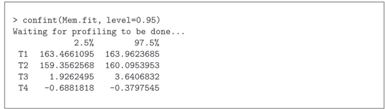
Example b from Membrane Separation Technology. As 5.a shows, from the profile t-plot we can graphically read out corresponding confidence intervals that are based on the profile t- function. TheRfunctionconfint(...) numerically calculates the desired confidence interval on the basis of the profile t-function.In Table 5.b is shown the corresponding R output from the membrane separation example. In this case, no large differences from the classical calculation method are apparent.

(17)

16 5. Profile t-Plot and Profile Traces

> confint(Mem.fit, level=0.95) Waiting for profiling to be done...

2.5% 97.5%

T1 163.4661095 163.9623685 T2 159.3562568 160.0953953 T3 1.9262495 3.6406832 T4 -0.6881818 -0.3797545

Table 5.b:Membrane separation technology example: Routput for the confidence intervals that are based on the profile t-function.

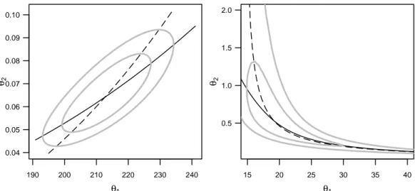
c Likelihood Profile Traces. The likelihood profile traces are another useful tool.

Here the estimated parameters θ^e_j, j 6= k at fixed θ_k (see 4.d) are considered as functions θ^e^(k)_j hθki of these values.

The graphical representation of these functions would fill a whole matrix of diagrams, but without diagonals. It is worthwhile to combine the ”opposite” diagrams of this matrix: Over the representation of θ^e^(k)_j hθ_ki we superimpose θ^e^(j)_k hθji – in mirrored form, so that the axes have the same meaning for both functions.

In Figure 5.c ist shown each of these diagrams for our two examples. Additionally, are shown contours of confidence regions for [θ₁, θ₂]. We see that the profile traces cross the contours at points of contact of the horizontal and vertical tangents.

The representation shows not only the nonlinearities, but also holds useful clues for how the parameters influence each other. To understand this, we now consider the case of a linear regression function. The profile traces in the individual diagrams then consist of two lines, that cross at the point [θ^b₁,θ^b₂]. We standardize the parameter by using δ_khθki from 5.a, so we can show that the slope of the trace θ^e^(k)_j hθki is equal to the correlation coefficient c_kj of the estimated coefficients θ^b_j and θ^b_k. The ”reverse

−3

−2

−1 0 1 2 3

190 200 210 220 230 240

δ(θ1)

T1(θ1)

θ1

−2 0 2 4

0.99 0.80 0.0 0.80 0.99

Level

−4

−2 0 2 4

20 40 60 80 100

δ(θ1)

T1(θ1)

θ1

0 10 20 30

0.99 0.80 0.0 0.80 0.99

Level

Figure 5.a:Profilet-plot for the first parameter is each of the Puromycin and oxygen consumption examples. The dashed lines show the applied linear approximation and the dotted line the construction of the 99% confidence interval with the help of T1hθ1i.