for dynamics of stochastic models and thermodynamics of fermionic models
I n a u g u r a l - D i s s e r t a t i o n zur
Erlangung des Doktorgrades
der Mathematisch-Naturwissenschaftlichen Fakult¨ at der Universit¨ at zu K¨ oln
vorgelegt von Andreas Kemper
aus Neuss
K¨ oln 2003
Priv.-Doz. Dr. A. Schadschneider Tag der m¨undlichen Pr¨ufung
5. November 2003
1. The TMRG Algorithm 9
1.1. Introduction . . . 9
1.1.1. Numerical Renormalization Group . . . 9
1.1.2. Density-Matrix Projection . . . 10
1.1.3. The DMRG Algorithm . . . 12
1.2. The TMRG Algorithm . . . 14
1.2.1. The Transfer-Matrix Formalism . . . 14
1.2.2. Implementation of the Algorithm . . . 20
1.2.3. Technical Remarks . . . 25
2. Extended Hubbard Models 28 2.1. Introduction . . . 28
2.2. Quantum Liquids in One Dimension . . . 32
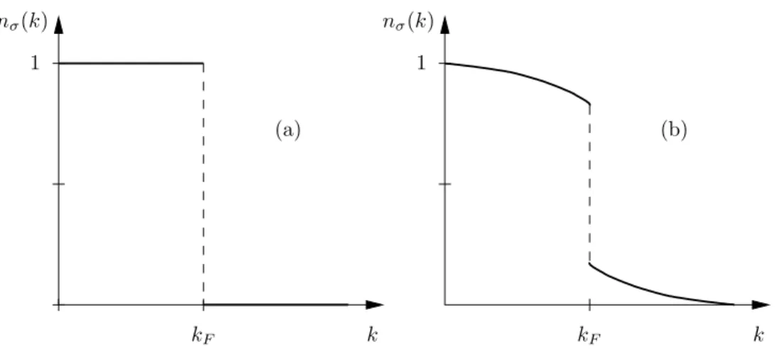
2.2.1. The Collapse of Fermi Liquid Theory . . . 32
2.2.2. Tomonaga-Luttinger and Luther-Emery Liquids . . . 34
2.2.3. Correlation Functions . . . 37
2.3. The Hirsch Model . . . 38
2.3.1. Introduction . . . 38
2.3.2. Bosonisation Predictions forX 1 . . . 40
2.3.3. The Exactly Solvable CaseX= 1 . . . 41
2.3.4. The Non-Integrable Regime 0< X <1 . . . 44
3. TMRG Results for the Hirsch Model 47 3.1. Introduction . . . 47
3.1.1. The Problem of Fermion Statistics . . . 47
3.1.2. Quantum Numbers and Correlation Lengths . . . 48
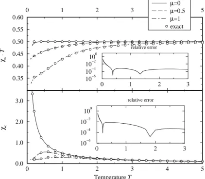
3.2. Thermodynamics of the Hirsch model . . . 49
3.2.1. TMRG Results forX = 1 . . . 51
3.2.2. TMRG Results for 0< X <1 . . . 53
3.3. Correlation Lengths . . . 61
3.3.1. Conformal Field Theory Predictions . . . 61
3.3.2. TMRG Results for Correlation Lengths . . . 64
4. Stochastic Models 68 4.1. Introduction . . . 68
4.2. The Master Equation and Quantum Formalism . . . 70
4.2.1. Asynchronous Dynamics . . . 71
4.2.2. Synchronous Dynamics . . . 72
4.3. Non-Equilibrium Criticality and Universality Classes . . . 73
4.4. Reaction-Diffusion Models . . . 75
4.4.1. The Diffusion-Annihilation Process . . . 75
4.4.2. The Branch-Fusion Process . . . 76
5. Stochastic TMRG 77 5.1. The Stochastic TMRG Algorithm . . . 77
5.2. Properties of the Stochastic Transfer-Matrix . . . 80
5.3. The Choice of the Density-Matrix . . . 83
5.4. Applications . . . 84
6. The Light-Cone CTMRG Algorithm 87 6.1. Introduction . . . 87
6.2. The Traditional CTMRG Algorithm . . . 88
6.3. The Concept of the LCTMRG . . . 90
6.4. The Choice of the Density-Matrix . . . 93
6.5. Some Technical Aspects . . . 94
6.6. Applications . . . 95
6.6.1. LCTMRG Results for the Diffusion-Annihilation Process 96 6.6.2. LCTMRG Results of the Branch-Fusion Process . . . 96
7. Conclusions 102 A. Jordan-Wigner Transformation 106 A.1. Spinless Fermions . . . 106
A.2. Fermions with Spin . . . 107
B. Exact Thermodynamics of the Hirsch model at X/t= 1 109 C. Correlation Lengths of Free Fermions with Spin 111 Bibliography 114 Danksagungen 121 Anh¨ange gem. Promotionsordnung 123 English Abstract . . . 123
Deutsche Kurzzusammenfassung . . . 125
Erkl¨arung . . . 127
Lebenslauf . . . 129
Strongly correlated systems with a huge number of degrees of freedom appear in many physical research fields, that reach from quantum models, statistical sys- tems to non-equilibrium phenomena. Typically, microscopic strong interactions can lead to highly non-trivial collective macroscopic behavior, which provides a fascinating field for theoretical studies.
The present thesis focus on two different types of one-dimensional strongly correlated systems that seemingly belong to opposed research fields. In the first part we study the thermodynamics of a fermionic model and thereby face typical questions of equilibrium physics. The second part of the thesis turns to investigations of stochastic systems, a quite modern research field of non- equilibrium physics.
On a theoretical level, strongly correlated systems are – even though they con- cern such different physics mentioned above – tractable by similar techniques.
Particularly interesting is the case of one dimension. On the one hand, the restricted topology alludes to a number of powerful analytical and highly pre- cise numerical methods. On the other hand, fluctuations and collective effects are generically strong. Therefore principle correlation effects are often studied in one dimension first, even if the original physical model necessitates a richer topology.
Since a couple of years, the rapid evolution of computer technology affected great progress in the development of complex numerical algorithms. One of the most important ones is the density-matrix renormalization-group (DMRG), which was developed by Whitein 1992 [1, 2] to study the low-energy physics of one-dimensional quantum systems. The DMRG is based on a surprisingly simple, but effective concept. The aim of the algorithm is to successively enlarge a Hamilton operator and store the respective matrix by a computer. The prob- lem of an exponentially increasing matrix dimension is countered by a renor- malization procedure, that integrates out physically “unimportant” degrees of freedom.
The discovery of the DMRG also initiated wide activity on various considerable variants of the method in other physical fields. For the numerical studies of the present thesis we use the so-called transfer-matrix DMRG (TMRG), that was originally introduced byNishinoin 1996 [3] to studytwo-dimensional classical statistical models.
In our case such a “second” additional dimension occurs in natural manner by the (reciprocal) temperature. It was indeed shown by Suzuki [4], that the thermodynamics of a one-dimensional quantum system with short-range interactions can be mapped onto a two-dimensional classical statistical model.
As he used a mathematical decomposition formula tracing back to Trotter
[5], the mapping is known as Trotter-Suzuki decomposition. After all, Xiang et. al [6, 7] noticed, that the TMRG algorithm thereby is suited to analyze also thermodynamic properties.
We will use the TMRG to study the thermodynamics of strongly correlated interacting fermion systems. Since the discovery of high-temperature super- conductivity byBednorzand M¨uller [8], the research in that field regained a great interest in solid state physics. A kind of minimal discrete model, that describes electrons moving in a narrow band and interacting by a strong (repuls- ive) Coulomb interaction, is the Hubbard model [9, 10, 11]. Here, the Coulomb coupling is reduced to an on-site repulsion termU, which is physically justifiable due to screening effects in a solid.
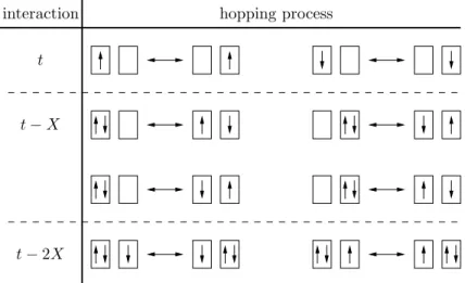
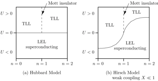
But recently models, that involve additional “longer ranging” two site terms of the Coulomb repulsion, have been intensively discussed, since the Hubbard model seems to be not a minimal model for some physical materials, e.g. poly- acetylene [12] or the Bechgaard salts [13]. Generally, these models are called extended Hubbard models. An interesting one has been proposed by Hirsch in 1989 [14], consisting of a bond-charge interaction term, which is also called correlated hopping. Based on a BCS-type theory he and Marsiglio showed [15, 16, 17, 18] that his model can lead to an effective attraction of holes in a nearly filled band and thus to (hole) superconductivity.
In a first part of the thesis we present a detailed thermodynamic study of the one-dimensional Hirsch model, using the TMRG algorithm. Even though some research was already done here for vanishing temperature T = 0, finite tem- peratureT >0 properties are almost unknown. We especially focus on the nu- merical calculation of thermal correlations, which is a fairly new field of TMRG research. The aim is to elucidate the model’s tendency to superconductivity for finite temperatures.
Our work with the TMRG algorithm also leads to intensive contentions with the method inherently. A completely different application field came into consid- eration: stochastic models which describe physics “far away” from the thermal equilibrium. Such non-equilibrium processes are found in several pure physical, but also many interdisciplinary fields, e.g. chemical reactions [19], traffic on a highway [20], etc. Generically, stochastic models stand to reason, if the micro- scopic dynamics are not exactly known, but empirical transition probabilities are available.
Strong correlation effects are also of central interest here, especially in low dimensions. But the theoretical framework of non-equilibrium collective phe- nomena is less elaborated than in the equilibrium counterpart. The typical numerical way to investigate stochastic models are (Monte-Carlo) simulations.
This means nothing else than randomly generating and averaging over possible configurations of the model. Even though this is a nicely simple and powerful numerical technique, a number of problems are known particularly at criticality (e.g. critical slowing down).
Considerable theoretical progress was made, as Alexander and Holstein [21] found out, that the master equation of (certain) stochastic models can be mapped onto a Schr¨odinger equation in “imaginary time”. The close analogy facilitates – at least formally – the adaption of quantum mechanical theories to
the stochastic case, e.g. the definition of a stochastic Hamiltonian or concepts like criticality, universality, conformal invariance, scaling, etc.
Inspired by the close relationship between quantum and stochastic models, the idea came up to apply the TMRG to non-equilibrium physics. Instead of the (reciprocal) temperature, the time represents the second dimension of the Trotter-Suzuki decomposition, if it is applied to the time evolution operator.
At first glance, this analogy seems to be rather close. But the contrast of the physics manifest itself in astonishingly exceptional properties of the so-called
“stochastic TMRG”. The non-equilibrium, time-dependent nature of stochastic models leads to a kind of causal structure, that considerably influences the algorithm and unfortunately leads to inherent numerical problems.
The second part of the thesis therefore proposes a new TMRG based algorithm for stochastic models, which we call – due to the causal structure – stochastic light-cone corner-transfer matrix DMRG (LCTMRG). This method is based on a corner-transfer-matrix approach, similary as introduced by Nishino and Okunishi in the context of classical two-dimensional systems [22, 23]. By means of feasibility studies of two well-known reaction-diffusion models we will judge about the numerical precision of the LCTMRG. Additionally we clarify the advantages arising from an approach, which is not a simulation technique and speculate about its future prospects.
Layout of the Thesis
Chapter 1 starts with a detailed overview of White’s density-matrix renor- malization-group (DMRG) algorithm in its historical context (section 1.1). We then discuss how the DMRG concept is transfered onto the thermodynamic case and elucidate the TMRG algorithm (section 1.2). Two variants are presented, the “traditional algorithm” following worksXiang et al. [6, 7] and a novel one proposed bySirker and Kl¨umper[24, 25].
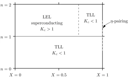
Chapter 2first reviews Hubbard’stight-binding approximation of fermions in a Coulomb potential (section 2.1), that provides the theoretical basis for the extended Hubbard models. Due to the restricted topology, one-dimensional fer- mion systems are usually described byTomonaga-Luttinger and Luther- Emery liquid theory, whose basic properties are summarized (section 2.2) and build the theoretic framework for the interpretation of our numerical results as well. Then we focus on the special extended Hubbard model concerned in this thesis, namely the Hirsch model (section 2.3), and review its current state of research.
Chapter 3presents our numerical computations for the Hirsch model. First, we mention some important details, how the “standard” TMRG algorithm is correctly applied to fermion systems (section 3.1). Then, TMRG data for the thermodynamics are shown and discussed in comparison with previous works (section 3.2), including also a precision check of the method. The chapter closes with an analysis of thermal correlation functions (section 3.3).
In Chapter 4 we turn to the world of non-equilibrium physics (section 4.1), which represents the second part of the present thesis. We focus on stochastic
processes in continuous time, but also sketch the discrete time case (section 4.2). Then, we review some conceptual facts about non-equilibrium criticality and universality classes (section 4.3). The chapter closes with an introduction of a particular class of stochastic models, namely reaction-diffusion processes (section 4.4), since they will be studied numerically later on.
Chapter 5outlines the stochastic TMRG algorithm, that is an almost one-to- one adaption of the quantum TMRG method onto the stochastic case. After displaying the specialties of the algorithm (section 5.1), important properties of the stochastic transfer-matrix (section 5.2) and the density-matrix projection (section 5.3) are discussed. Finally we point out principal numerical instabilities that restrict the method’s capability (section 5.4).
Chapter 6 introduces the newly proposed stochastic light-cone CTMRG al- gorithm. On the basis of corner-transfer-matrices (section 6.2) we outline the concept of the LCTMRG method (section 6.3), focusing on the most crucial part of choosing the correct density-matrix projection (section 6.4) and alluding to some additional technical details (section 6.5). Finally we exemplary investig- ate two well-known reaction diffusion models using the LCTMRG (section 6.6).
Hereby, our aim is to judge the quality of the numerical results.
Chapter 7 draws the conclusion of this thesis and proposes perspectives for further research on the presented topics.
1.1. Introduction
The density-matrix renormalization group (DMRG), which was developed by White in 1992 [1, 2], is one of the most precise numerical methods to study low-dimensional strongly correlated systems. Originally, it was introduced to compute the ground state and low-energy spectrum of a quantum Hamiltonian with short-range interactions. But meanwhile, there is a large number of vari- ants using the basic DMRG idea of numerical renormalization in other physical fields, see e.g. [26] as a general reference. One of these variants is the transfer- matrix DMRG (TMRG) which can be used to study the thermodynamics of (quasi) one-dimensional quantum systems.
In this section we give an overview of the DMRG and TMRG algorithms in a historical context. The DMRG is an advancement of Wilson’s numerical renormalization group method (NRG), that is outlined in section 1.1.1. White augmented the NRG by the density-matrix projection (section 1.1.2) that is the basic idea of each DMRG-style method. Thereupon, in section 1.1.3 the
“standard” DMRG algorithm is presented. The TMRG algorithm, which we review in section 1.2, is an adaption of the DMRG concept to the so-called transfer-matrix. A detailed overview about the algorithmic realization is given, following works of Xianget al. [6, 7] and Sirkerand Kl¨umper[24, 25].
1.1.1. Numerical Renormalization Group
The RG was first proposed by Wilson in 1971 to study critical phenomena of quantum systems [27]. This original RG was based on the idea, that large length scales dominate the physics at criticality and thus microscopic lengths are renormalized. Wilson also first applied a pure numerical RG variant (NRG) to theKondomodel and computed the ground state [28].
Figure 1.1 outlines Wilson’s NRG approach. The algorithm starts with a quantum chain (also called “block”) of length L, that is sufficiently small to be numerically represented on a computer. Then, the Hamiltonian HL is en- larged sequentially by one site to increase the system size. In order to reduce the exponentially growing dimension of the Hilbert space, HL is renormalized after each enlargement step by retaining only afixed numbermof Hilbert space states. All remaining states are cut off and neglected for the next iteration step.
Obviously the crucial question arises which states are in that sense “relevant”
to find an optimal truncation procedure. In Wilson’s NRG the Hamiltonian is diagonalized to keep only themstates of lowest-energy. Alternating the renor- malization and enlargement step, the “effective” block size thereby is increased,
H¯L
H¯L+1
Renormalisation H¯L
HL+1 Enlargement of Chain
Figure 1.1.: Schematic plot of Wilson NRG method.
while the Hamilton operator of dimension m×m is kept representable by the computer algorithm.
The key problem of this RG method is, that the energetically lowest eigenstates are assumed to be an optimal renormalization basis for the ground state. In the Kondo problem this situation is indeed realized. But applications of the NRG to e.g. the Heisenberg or Hubbard model do not provide this feature. Here, the NRG provides only poor numerical results for the ground state [29, 30].
1.1.2. Density-Matrix Projection
The problem, which states are relevant in a RG step to represent the ground state, was solved by White’s density-matrix (DM) projection. This section pre- sents a detailed mathematical formulation of the DM projection [31], which is the basis of all “DMRG-like” algorithms.
We start with the block Hamiltonian HL=
LX−1 i=1
hi,i+1 (1.1)
of chain length L and next-neighbor interactionshi,i+1, operating on a Hilbert spaceHs. The idea of the DM projection is to embedHLinto a larger quantum chain. This is typically done by mirroringHL to construct the so-called super- block
Hsuper=HL⊗idL+hL,L+1+ idL⊗HL . (1.2) Figure 1.2 depicts the superblock, which is split up into the so-called system block Hs and environment block He. The DM projection is designed to com- pute a small set of m < k := dimHs states ui
∈ Hs (i = 1. . . m) which are important to represent the ground state (also called target state) of the superblock
ψ
=X
ij
ψiji
s⊗j
e. (1.3)
superblock
V U
Hs He
environment block system block
Figure 1.2.: Schematic diagram of the superblock, that consists of a system and environment block.
Here, i
s (i= 1. . . k) and j
e (j = 1. . . k) label an orthonormal basis of the Hilbert spaceHs andHe, respectively.
The problem of finding optimal representation vectorsui
can be mathematical formulated as follows: Find an optimalm-dimensional subspaceU∈Hs and a vector
ψ˜
=X
ij
ψ˜ijui
s⊗j
e∈U⊗He, (1.4)
that minimize the functional S ψ˜
:=ψ
−ψ˜2 . (1.5)
We show, that the optimal ui
are given by the eigenvectors of the leading eigenvalues of the reduced DM
ρ:= tr0ψ
ψ , (1.6)
where tr0 := ids⊗tre labels the partial trace over the environment block. We interpret the coefficientsψijand ˜ψij ask×kmatricesψ= (ψij)ij and ˜ψ= (ψij)ij (where rank( ˜ψ)≤m) respectively. Then, the DMρ can be written as ρ=ψψ† and the functionalS(ψ˜
) turns to
S( ˜ψ) = tr (ψ−ψ)˜ †(ψ−ψ)˜ . (1.7) Using the singular value decomposition theorem (SVD) [32] one can simplify equation (1.7). According to the SVD there exist two orthogonalk×kmatrices U and V such that
ψ=U DV† , whereby D= diag(σ1, . . . , σk,0, . . . ,0). (1.8) The so-called singular values σi are the square roots of the eigenvalues ρi ofρ, because
ρ=U DD†U†=U D2U† . (1.9) Without loss of generality the σi are sorted: σ1 ≥ σ2 ≥ · · · ≥ σk. Inserting (1.8) into (1.7) we obtain
S( ˜ψ) = tr (D−D)˜ †(D−D)˜ . (1.10)
whereby ˜D := U†ψV˜ . Obviously, S is minimized by a diagonal matrix ˜D of rank m, whose diagonal elements are given by the leading singular values, i.e.
D˜ = diag(σ1, . . . , σm,0, . . . ,0) . (1.11) Hence, we can explicitly constructψ˜
which minimizesS:
ψ˜
= X
ij
(UDV˜ †)iji
s⊗j
e=X
ij
D˜ij Ui
| {z }s
ui
⊗ Vj
| {z }e
vj
= Xm i=1
σiui
s⊗vi
e (1.12)
The vectorsui
e (i= 1. . . m) are the leading eigenvectors ofρ, cf. eq. (1.9).
We have proved that the relevant states of the system block to represent the ground state of a larger quantum chain are optimally given by the leading eigenvectors of the reduced DM. Note, that also the environment block has been automatically projected to a subspaceV= span{vi
e}, cf. figure 1.2.
The truncation error made by cutting off the subspaceU⊥ can be measured by the so-called discarded weight
P := 1− Xm i=1
ρi. (1.13)
The faster the ρi decrease, the better normally the renormalization step per- forms. Thus, the DM spectrum is a good indicator for the quality of the DM projection. For some integrable models the DM spectrum can be obtained exactly [33], typically showing a fast exponential decay.
Without going into the details we also mention that other types of DM are possible depending on which states have to be targeted. E.g. in order to compute the excitation spectrum’s gap of a quantum system, not only the ground state ψ0
, but also the first exited stateψ1
should be involved in the reduced DM, namely
ρ= 1
2tr0 ψ0
ψ0+ψ1
ψ1. (1.14)
1.1.3. The DMRG Algorithm
We focus here on the so-calledinfinite size DMRG algorithm. As a counterpart we mention thefinite size algorithm [34], which is not used in this work. Often, both algorithms are combined to obtain an increased accuracy of the numerical results.
The infinite size algorithm is designed for computing the ground state (or low- energy spectrum) of a quantum chain in the thermodynamic limit L → ∞. It contains the following iterative steps:
1. Construct and store the system block of size L Hs=
L−1
X
i=1
hi,i+1= . (1.15)
If any (local) expectation value is desired to be measured, store the matrix A=
XL i=1
ai (1.16)
with ai being an arbitrary local operator of sitei.
2. Enlarge the system block by one site
H˜s=Hs⊗id +hL,L+1 = (1.17)
and similarly the expectation value operator
A˜=A⊗id +aL+1 . (1.18)
3. Construct the superblock
Hsuper= ˜Hs+hL+1,L+2+ ˜He
H˜s H˜e
where the environment block ˜He is obtained by mirroring the system block ˜Hs. Compute the ground stateψ
(and excitations where required) numerically.
4. Compute the reduced density-matrix ρ and its complete eigenspectrum {ρi,ui
}. Write the orthonormal eigenstates of themleading eigenvalues into a matrix U.
5. Compute all local expectation values
hAi= trρA .˜ (1.19)
6. Project all operators onto the reduced basis using the operatorU, i.e.
Hs=U†H˜sU, A=U†AU˜ (1.20) Hs
and continue from step 2.
Obviously, the chain length grows successively by each iteration step, whereas the effective size of the system’s Hamiltonian stays constant. By finite size analysis, highly precise estimates of various properties of the infinitely large quantum chain are possible.
The scheme given above is only a rough sketch of the DMRG algorithm. An implementation of a DMRG program facilitates various numerical know-how to increase the performance and to save computer memory. Typically, quantum numbers reduce operators to a block structure, such that vanishing matrix elements do not have to be stored. The most time consuming part of the algorithm is found in the computation of the ground state. Here, theDavidson [35] orLanczos[36] algorithm are typically used due to their high performance.
1.2. The TMRG Algorithm
In general, all thermodynamic quantities of a d dimensional quantum system can be derived analytically from the partition function
Z = tr
e−βH
=X
i
e−βEi . (1.21)
Hence, in principle one has to diagonalize the Hamiltonian to obtain the whole spectrumEi, which is analytically impossible in most cases. It is also a hopeless way to compute the whole spectrum numerically due to the large dimension of the Hilbert space.
A promising alternative approach is given by the Trotter-Suzuki decom- position [5, 4, 37], where the quantum system is first mapped onto a classical two-dimensional lattice, cf. fig. 1.3. The classical system is then solved in terms of a transfer-matrix formulation, which we describe in detail in section 1.2.1.
As a crucial result it is found, that the thermodynamics of the quantum chain are determined by the leading eigenvalue Λ0 of the so-called quantum transfer- matrix (QTM).
solves decomposition
classical system solution of classical system d+ 1 dimensional
thermodynamics
Trotter Suzuki quantum system
ddimensional
transfer matrix formalism complete
eigenspectrum
Figure 1.3.: Schematic plot of the Trotter-Suzuki decomposition.
For some integrable models (such as the Hubbard model [38] or the supersym- metric tJ model [38, 39]) Λ0 can even be calculated analytically. For arbitrary models the TMRG algorithm introduced by Xiang et al. provides a precise numerical technique to obtain Λ0, which is nothing else than the consequent adaption of the DMRG onto the QTM. The concepts of the algorithm are sum- marized in section 1.2.2. Finally, we focus on some details of the numerical implementation in section 1.2.3, which are important for a successful realiza- tion of a TMRG computer program.
1.2.1. The Transfer-Matrix Formalism
Our starting point is an arbitrary one dimensional Hamiltonian H =
XL i=1
hi,i+1 (1.22)
of length L with periodic boundary conditions hL,L+1 = hL,1. H acts on a Hilbert space H = h⊗i of a one-dimensional quantum chain. Withh we label the local Hilbert space of site iwith dimension n= dimh. We further assume that the local interactionhi,i+1 conserves parity, i.e. hi,i+1 =hi+1,i.
In this section, we present two different Trotter-Suzuki mappings. The first one is the basis of the “traditional” quantum TMRG algorithm introduced byXiang et al. [6, 7]. The second one was first used for TMRG bySirkerandKl¨umper [24, 25] and has some advantages and disadvantages, which we describe later on.
In the traditional mapping the interactions of the Hamiltonian are split up into an odd and an even part
Ho= X
iodd
hi,i+1, He= X
ieven
hi,i+1, H =Ho+He. (1.23) The partition function is then expressed by theTrotter formula [5]
Z = tr
e−βH
= lim
M→∞
e−Hoe−He M
, (1.24)
where = β/M. If we omit the limit M → ∞ and fix , the Trotter formula approximates the partition function
Z = tr
e−Hoe−He M
+O(2) , (1.25)
whereby one can show, that the error is of the orderO(2) [25].
A fixedthereby discretizes the temperature T = 1
M . (1.26)
Inserting 2M identity operators into the partition function yields
Z = X
{α}
α1e−Hoα2
α2e−Heα3
· · ·
×
α2M−1e−Hoα2M
α2Me−Heα1
. (1.27)
Here, the vectors
αj
= OL
i=1
sij
∈H, j = 1. . .2M (1.28) are tensor products ofsij = 1. . . n, which denote a local orthonormal basis ofh. AsHo and He consist of commuting local interactionshi,i+1 only, they resolve into a product
e−He/o = Y
ieven/odd
e−hi,i+1 . (1.29)
Therefore, the partition function can be written as Z=X
{s}
τ11,,22τ13,,24· · ·τ1L,−12 ,L
τ22,,33τ24,,35· · ·τ2L,,31
· · · (1.30)
× τ21M,2−1,2M· · ·τ2LM−1−1,L,2M
τ22M,,31· · ·τ2LM,−11,L ,
where we used τj,ji,i+1+1 as an abbreviation of the tensor elements τj,ji,i+1+1:=
sijsij+1e−hi,i+1sij+1sij+1+1
. (1.31)
The expression (1.30) is a kind of lattice path integral representation of the partition functionZ. This is visualized in figure 1.4, which shows a checkerboard style lattice.
M = 3
M = 2
M = 1
M dimension
Trotter
quantum dimensionL
Figure 1.4.: Schematic plot of the two-dimensional classical lattice of the Trotter-Suzuki decomposition. The figure shows the special case of Trotter dimensionM = 3.
The sites of the lattice, given by the basis statessij, interact by local plaquettes
τj,ji,i+1+1 =
sij si+1j si+1j+1 sij+1
. (1.32)
Here we used a special pictorial representation of the plaquettes to allude par- ticularly to the symmetries:
τj,ji,i+1+1 =τji,i+1+1,j (hermicity) (1.33) τj,ji,i+1+1 =τj,ji+1+1,i (parity conservation) . (1.34) One can now easily conclude by equation (1.30), that Z corresponds to the partition function of the shown two dimensional model with classical spins sji. Hence, the quantum dimension L has been expanded by a virtual Trotter dimensionM, taking the role of the imaginary time of the lattice path integral.
Note, that the Trotter-Suzuki decomposition also leads to periodic boundary conditions in Trotter directionM.
The key point of the TMRG is that the classical model provides the ther- modynamics of the quantum model. Consequently, we rather solve the two- dimensional classical models, which is done in terms of a transfer-matrix form- alism.
We define the so-called quantum transfer-matrix (QTM) TM with matrix ele- ments
{si}TM{si+2}
= X
{si+1}
τ1i,i,2+1τ3i,i,4+1· · ·τ2i,iM+1−1,2M
× τ2i+1,3 ,i+2τ4i+1,5 ,i+2· · ·τ2i+1M,,i1+2
= ... ...
...
si1 si2 ...
si3 si2M
si+22 si+23 si+22M si+21
(1.35)
Here, a column of the lattice was joined for the construction ofTM (cf. figure 1.4). Due to a (two site) translational invariance inL direction, TM does not depend oni. Hence, we abbreviate eq. (1.35) by
TM = τ1,2τ3,4· · ·τ2M−1,2M
· τ2,3τ4,5· · ·τ2M,1
. (1.36)
Now equation (1.30) takes the simple form Z = trTML/2 =X
µ
ΛL/µ 2 . (1.37)
The eigenspectrum ofTM, denoted by Λµ, is not necessarily real. As one can imagine by the shape of TM in eq. (1.35), TM is in general not symmetric.
Moreover, left and right eigenvectors (i.e. those of TM and TM† , respectively) have to be distinguished.
The eigenvalues are now assumed to be sorted, i.e.|Λµ| ≥ |Λµ+1|. The leading eigenvalue Λ0 is usually not degenerate and we have a finite gap Λ0 6= Λ1. This can be explained by considering the high temperature caseT → ∞, where
τj,ji,i+1+1=δsi
j,sij+1δsi+1
j ,si+1j+1 = (1.38)
becomes unity.
Giving a pictorial proof in fig. 1.5 we can show
TM2 = n2TM and (1.39)
trTM = n2 . (1.40)
= =
trTM n2 TM2 n2 · TM
Figure 1.5.: Pictorial proof of eq. (1.39) and (1.40). The figure shows the trace ofTM and its second powerTM2 . Since the local plaquettes are unity, the “connected” indices have to be equal. The summation over a
“column” of such indices, depicted by curved lines, contributes by a factor ndue to nlocal spin configurations.
From eq. (1.39) it is evident that Λµ=n2 or Λµ= 0. Then, eq. (1.40) determ- ines the spectrum
specTM =
n2,0, . . . ,0 (1.41) and verifies a gapped transfer-matrix at infinite temperatures. Since a phase transition is not possible for one-dimensional quantum systems with short range interactions, the gap is expected to persist for any finite temperatureT >0.
Equation (1.37) is nicely suited to perform the thermodynamic limitL→ ∞ of the quantum dimension exactly. For largeL we find
TML/2 =P
µΛL/µ 2ΛRµ
ΛLµ −−−−→L→∞ ΛL/0 2ΛR0
ΛL0 (1.42) and
Z −−−−→L→∞ ΛL/0 2 . (1.43) Consequently, the free energy per site in the thermodynamic limit reduces to depend only on the leading eigenvalue Λ0
f∞,M =−T lim
L→∞
1
LlnZ =−T
2 ln Λ0 . (1.44)
Note, thatf∞,M is still an approximation and does not represent the bulk limit f∞,∞ of the quantum chain. The “finite size” corrections due to M are (cf.
eq. (1.25))
f∞,M =f∞,∞+O(2). (1.45) It is well known, that the complete thermodynamics can be analytically derived from the free energy. But in the face of the later numerical algorithm based on the QTM approach, it is convenient to compute local observables in a different manner. We consider an arbitrary operator Oi,i+1, which acts on two neigh- boring sites iand i+ 1, and express
Oi,i+1
in the transfer-matrix formalism by
hOi,i+1i= 1
Z tr Oi,i+1e−βH
= 1
Z tr TM(O)TML/2−1
. (1.46)
Here,TM(O) denotes a modified QTM
TM(O) = τ1,2(O)τ3,4· · ·τ2M−1,2M
τ2,3τ4,5· · ·τ2M,1
(1.47) where one plaquetteτ1,2(O) embeds O
τ(O)i,ij,j+1+1 :=
sijsij+1Oi,i+1e−hi,i+1sij+1sij+1+1
. (1.48)
Note that in eq. (1.47) the indices ofOare omitted, becauseO can be measured at an arbitrary site due to translational invariance. For the thermodynamic limitL→ ∞, eq. (1.46) reduces to
hOi,i+1i= 1
Z tr TM(O)TML/2−1
L→∞
−−−−→ ΛL/0 2−1 ΛL/0 2
tr TM(O)ΛR0 ΛL0
=
ΛL0TM(O)ΛR0
Λ0 . (1.49)
In this thesis we also regard thermal two-point correlation functions GO(r) = hδO1δOri, where δOr =Or− hOri and Or is a one or two site operator. In a similar way to eq. (1.49) one obtains
GO(r) = tr δO1δOre−βH L→∞
−−−−→
ΛL0TM(δO)TMr/2−1TM(δO)ΛR0 Λr/0 2+1
=X
α6=0
ΛL0TM(δO)ΛRα
ΛLαTM(δO)ΛR0 Λ0Λα
| {z }
Mα
Λα Λ0
r/2
=:X
α
Mαe−r/ξαeikαr (1.50)
where we have introducedthermal correlation lengths (CL)ξαandwave vectors kα
ξα−1= 1 2ln Λ0
|Λα| and kα = 1 2arg
Λ0 Λα
mod π . (1.51) The asymptotic behaviorGO(r → ∞) is dominated by the largest CL ξα, for which the matrix elementMα does not vanish. Note, that due to the gap inTM the CLsξαare well defined. Moreover we conclude that all correlation functions GO decay exponentially.
The checkerboard lattice is translational invariant in space directionL, but only with a double unit cell. This complicates the calculation ofkα, since one can not distinguish betweenkα and kα+π. This problem was solved in the context of TMRG bySirkerand Kl¨umper, who used a different QTM [25, 24]. Instead of eq. (1.25) we write
Z = tr (T1T2)M/2 with T1/2 =TL/R
e−H+O(2)
(1.52) whereTL/R is the shift left and right operator, respectively. The corresponding lattice is shown in fig. 1.6 (a). In contrast to the checkerboard lattice, the
si1 si2 si3 ... si2M
... ...
si+21 si+22
translational invariant (a)
TM (b)
si+22M
si+23 ...
Figure 1.6.: Alternative Trotter-Suzuki decomposition of the thermodynam- ics. Figure (a) depicts the classical lattice, (b) the corresponding quantum transfer-matrix.
number of lattice sites per Trotter stepM has doubled. Consequently, we have to exchange by /2 to make both decompositions comparable. As another important difference, the lattice of fig. 1.6 (a) is obviously fully translationally invariant in quantum direction L. The corresponding QTM TM is shown in fig. 1.6 (b). As a consequence, the wave vectors kα in eq. (1.51) are unique.
Note, that additionally a factor 1/2 has to be omitted, e.g. in eq. (1.44) and (1.51).
We have shown in the current section, that the calculation of the thermodynam- ics reduces to finding the leading eigenvalues Λαof the quantum transfer-matrix.
In order to cover the whole temperature region it is necessary to increase M to lower the temperature (cf. eq. (1.26)). But the exponential dimensionn2M×n2M of the QTM TM generically prevents an exact treatment. Only in a few spe- cial case, the algebraic Bethe ansatz provides analytical solutions for Λ0 for arbitrary M.
A promising numeric tool was proposed by Xiang et al. in 1996 [6, 7], which applies the DMRG algorithm onto the QTM and therefore is called (quantum) transfer-matrix DMRG (TMRG).
1.2.2. Implementation of the Algorithm
In principle, the TMRG algorithm is nothing else but the application of the DMRG method (cf. sec. 1.1) onto the quantum transfer matrixTM. Whereas the DMRG is basically designed for computing theground state andlow excitations, respectively, the TMRG computes the leading part of the spectrum.
Historically, a numerical TMRG algorithm was first introduced by Nishinoin 1995 [3] in the framework of classical two-dimensional systems. Xiang et al.
transfered their ideas to the thermodynamic case [6, 7]. Even if the basics of
the TMRG are closely related to its DMRG predecessor, the rich structure of the transfer-matrices turns the algorithm to be slightly more sophisticated.
Traditional TMRG Algorithm
First, we discuss the “traditional” TMRG method of Xiang et al. In order to exemplify the renormalization process we consider two special casesM = 3 and M = 4 (because odd and even Trotter numbers are handled slightly different).
Schematically, the (infinite) TMRG algorithm proceeds by the following itera- tions steps:
1. Construct the system block S =
(
(τ1,2τ3,4· · ·τM,M+1)(τ2,3τ4,5· · ·τM−1,M) ifM odd
(τ1,2τ3,4· · ·τM−1,M)(τ2,3τ4,5· · ·τM,M+1) ifM even (1.53) and environment block
E= (
(τM+2,M+3· · ·τ2M−1,2M)(τM+1,M+2· · ·τ2M,1) if M odd
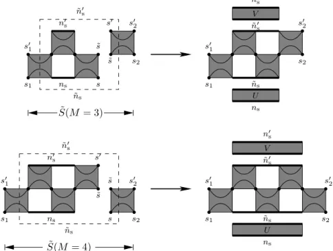
(τM+1,M+2· · ·τ2M−1,2M)(τM+2,M+3· · ·τ2M,1) if M even (1.54) respectively, which are depicted in fig. 1.7. We write the tensors S andE
S(M = 4)
E(M = 3) S(M = 3)
E(M = 4) T(M = 4) =
T(M = 3) =
n0e n0s
n0e n0s
s02 s01
˜ s1
ne
˜ s1
s2
˜ s2
˜ s2
˜ s2 ns s1
s01
s2
˜ s1 s02
˜ s1
ne
˜ s2
ns s1
Figure 1.7.: System and environment block in the TMRG algorithm for the special casesM = 3 and M = 4.
in a basis representation
Sss01n0ss02
1nss2
and
Ess01n0es02
1nes2
. (1.55)
Here, thes-indices label single spin sites, whereas then-indices joinM−1 spins to a block spin. Thus, the dimension of S and E is n4·m˜2 with
˜
m=n2(M−1).


![Figure 2.8.: The figures are taken from numerical calculations of Quaisser [79].](https://thumb-eu.123doks.com/thumbv2/1library_info/3707962.1506242/45.892.158.714.219.730/figure-figures-taken-numerical-calculations-quaisser.webp)