Genotyping by sequencing
from sparse sequenced genomes representations from bi- and multi- parental mapping population
using a HMM approach
Inaugural-Dissertation zur
Erlangung des Doktorgrades
der Mathematisch-Naturwissenschaftlichen Fakultät der Universität zu Köln
vorgelegt von
Vipul Kumar Patel aus Dortmund
Köln
2016
Die vorliegende Arbeit wurde am Max-Planck-Institute für Züchtungsforschung in Köln in der Abteilung für Entwicklungsbiologie der Pflanzen (Direktor Prof.
Dr. George Coupland) angefertigt.
Berichterstatter: Prof. Dr. George Coupland (Gutachter) Prof. Dr. Achim Tresch Prüfungsvorsitzender: Prof. Dr. Marcel Bucher
Tag der mündlichen Prüfung: 18.April.2016
Abstract
Genotyping is one key element for successfully carrying out molecular breeding, gene network discovery or assessment of genetic diversity. The onset of next generation sequencing has enabled high-resolution genotyping of thousands or millions of markers per individual in one analysis. Such dense information can be used to identify genetic loci associated with a trait of interest. Development of multiplexing allows sequencing of whole populations in a single run, vastly reducing inputs of time and money per sample. This high throughput genotyping is known as genotyping-by-sequencing (GBS). However, there is a trade-off for using GBS, as the total number of reads per run must be distributed across all samples, leading to a reduction of coverage per sample. The distribution of the total reads is currently not uniform, which leads to samples with only partial sequence coverage.
This thesis presents a solution for handling such data by imputing missing markers based on a Hidden Markov Model approaches for bi- and multi- parental mapping populations. The developed methods were not only validated by simulation studies but also applied to several real mapping population datasets. For the bi-parental mapping population, data were derived from three different taxa (Arabidopsis thaliana, Sorghum bicolor and Fragaria vesca) and for the multi-parental mapping population the Arabidopsis multi-parental RIL (AMPRIL) population was genotyped.
The successful high resolution genotyping of such mapping populations with sparse sequencing data demonstrates the advantages of the developed method and the positive effects for downstream analysis e.g. for quantitative trait analysis or genome- wide-association studies.
This thesis additionally provides a theoretical approach and implementation for a
hybrid correction approach of sequencing errors in third generation sequencing data
from Pacific Biosciences.
Zusammenfassung:
Die Genotypisierung ist ein wichtiges Verfahren, insbesondere für eine erfolgreiche molekulare Züchtung, bei der Aufdeckung von Gennetzwerken oder der Ermittlung der genetischen Vielfalt einer Population. Besonders durch die Einführung von „Next- generation-sequenzierung“, gelang es Millionen von neuen und unbekannten
Markern pro Individuum zu genotypisieren. Die so gewonnene Informationsdichte erlaubt es, eine effektive Analyse der Beziehung zwischen Genen und deren Eigenschaften aufzudecken. Für solche komplizierten Analysen müssen mehrere hundert Individuen sequenziert werden, was einem hohen Investitionsaufwand entspricht. Mit der Einführung von „multiplexing“ wurde es möglich, Individuen gleichzeitig parallel zu sequenzieren und zu genotypisieren. Diese Methode wird als
„Genotyping by sequencing“ (GBS) bezeichnet. Sie hat aber den Nachteil, dass nicht alle Individuen gleichmäßig sequenziert werden. Es gibt somit Individuen, deren Genome nur teilweise sequenziert werden. Dies reduziert die Anzahl der Marker, welche genotypisiert werden können.
In dieser Arbeit stellen wir eine Lösung vor welche mit Hilfe eines statistischen Modells, dem „Hidden Markov Model“ fehlende Informationen vorhersagen kann. Es wurden zwei Modele entwickelt für Populationen von zwei oder mehr Eltern. Die entwickelten Methoden wurden mit simulierten Daten getestet und auf tatsächlich vorhandenen Population angewendet: für Populationen generiert aus zwei Eltern (Arabidopsis thaliana, Sorghum bicolor and Fragaria vesca) und für mehrere Eltern, die Arabidopsis multi-parental RIL Population. Die Anwendung unserer Methoden auf diese Populationen half, neue Erkenntnisse und Kandidatengene zu finden.
Zusätzlich zum Thema „Genotyping by sequencing“ wird ein Algorithmus behandelt,
welcher die Korrektur von langen Sequenzeninformation geeignet ist, die von der
Technologie Pacific Bioscience generiert wurden.
INTRODUCTION ... 1
H IGH - THROUGHOUT GENOTYPING ... 1
B ASIC CONCEPT OF II LUMINA SEQUENCING TECHNOLOGY ... 3
G ENOTYPING USING NGS GENOTYPING BY SEQUENCING (GBS) ... 3
G ENOTYPING BASED ON SPARSE SEQUENCING DATA . ... 4
I MPUTATION USING A SIMPLE SLIDING WINDOW APPROACH ... 5
H IDDEN -M ARKOV M ODEL (HMM) ... 6
1. GENOTYPING BY SEQUENCING FOR BI-PARENTAL CROSSES ... 8
1.1 M ETHOD ... 8
1.1.1 Premises for using the TIGER pipeline ... 8
1.1.2 Marker generation ... 8
1.1.3 Pre-assignment of genotypes at individual marker positions ... 9
1.1.4 State model of the HMM implemented in TIGER... 10
1.1.5 Parameter estimations for the Hidden-Markov Model (HMM) ... 11
1.1.5 Increasing the CO resolution by incorporating removed low quality markers ... 13
1.1.6 In-silico validation of TIGER ... 15
1.1.7 Errors detected during in-silico validation ... 16
1.2 RESULTS... 18
1.2.1 Applying TIGER on individuals of a mapping population of A. thaliana ... 18
1.2.1.1 Introduction ... 18
1.2.1.2 Reconstructions of wild type and recq4a F2 sample genomes ... 19
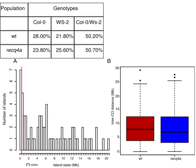
1.2.1.3 RECQ4a does not affect the frequency or distribution of CO events in Col-0 X Ws-2 F2 populations ... 24
1.2.1.4 A suppression of COs reveals a 1.8 Mb inversion ... 26
1.2.2 Applying TIGER on a Fragaria vesca mapping population ... 27
1.2.2.1 Strawberry genome ... 27
1.2.2.2 SNP markers filtering ... 27
1.2.2.3 Sequencing results for the 40 selected samples ... 28
1.2.2.4 GBS of the 40 strawberry recombinants ... 29
1.2.2.5 Evaluation and breakpoint resolution ... 31
1.2.2.6 Genotype frequency and QTL detection ... 32
1.2.3 GBS applied to a Sorghum bicolor mapping population ... 35
1.2.3.1 The S. bicolor genome ... 35
1.2.3.2 Plant material, SNP marker estimation and sequencing results... 35
1.2.3.3 Reconstruction of the mosaic structure for each sample ... 37
1.2.3.4 Detection of selection pattern ... 40
1.2.3.5 QTL-analysis ... 40
1.3 D ISCUSSION AND CONCLUSION ... 43
. . Appearance of islands ... 44
1.3.3 Future improvements ... 44
2. GENOTYPING MULTI-PARENTAL RIL POPULATIONS ... 46
2.1 I NTRODUCTION ... 46
2.2 M ETHOD ... 49
2.2.1 Resequencing the samples from the AMPRIL population using RAD-seq... 49
2.2.2 Assignment of genotypes at each marker positions ... 49
2.2.3 Two stage Hidden-Markov-Models... 50
2.2.4 Visualization of the allelic support of four parents ... 51
2.2.5 Simulations and training of the HMM ... 53
2.2.6 Genetic incompatibilities ... 53
2.3 R ESULTS ... 56
2.3.1 Resequencing results of the founder lines of the AMPRIL population ... 56
2.3.2 Resequencing the AMPRIL population ... 58
2.3.3 Validation with simulated data ... 60
2.3.4 Error position and type ... 61
2.3.5 Using technical replicates for testing of reproducibility ... 62
2.3.6 Genotype validation using 300 previously genotyped SNP markers ... 63
2.3.7 Outcross events ... 64
2.3.8 CO landscapes and genotype frequencies per sub-populations ... 65
2.3.9 Genetic incompatibilities ... 69
2.4 D ISCUSSION ... 71
2.4.1 Summary... 71
2.4.2 Improvements ... 72
2.4.3 Outlook ... 73
3. ERROR CORRECTION FOR LONG READS GENERATED WITH PACIFIC BIOSCIENCES SEQUENCING TECHNOLOGY ... 74
3.1 I NTRODUCTION ... 74
3.2 M ETHOD ... 76
3.2.1 Correcting Pacific Biosciences reads by using second generation sequencing data ... 76
3.3.4 Simulation studies ... 85
3.3.5 Error distribution and type of errors ... 85
3.4 D ISCUSSION ... 87
3.4.1 Improvements ... 87
4. OUTLOOK ... 89
4.1 T HE FUTURE PERSPECTIVE OF GBS ... 89
4.2 W OULD INCREASING THE READ LENGTH OF SHORT READ DATA HAVE AN IMPACT ON GBS? ... 89
4.3 W ILL IMPUTATION BE NEEDED IN THE FUTURE ? ... 89
4.4 T HIRD GENERATION SEQUENCING AND THEIR POTENTIAL . ... 90
ABBREVIATIONS ... 91
REFERENCES ... 93
DANKSAGUNGEN ... 101
ERKLÄRUNG ... 102
Introduction
Individuals share broadly the same DNA sequences, however, many of the homologous loci show different types of DNA sequences which are referred to as alleles. Genotyping is the process of characterizing the specific alleles within an organism, which can be natural differences or artificially induced mutations. Differentiating genotypes allows understanding sources of phenotypic variations. The individual genetic loci with different alleles underlying the variation in a phenotype are defined as quantitative trait loci (QTL). Hence, correlation between phenotypic and genetic variation can be used to identify regions coding for a particular phenotype or trait of interested.
Such knowledge than can be used for an effective breeding process or to unravel further downstream genetic networks.
However, complex trait analyses requires populations of more than hundreds or even thousand of individuals. For this amount of individuals applying standard genotyping methods are not
practicable and require huge investment. Next-generation-sequencing (NGS) allows to genotype more than thousand markers in a single run allowing to not only by-pass time-intense genotyping efforts but would also allow for the reconstruction of recombination breaks at great resolution. In combination with multiplexing multiple individuals can be sequenced in parallel. This reduces the sequencing cost per individual, but comes at the price of having only partial genomes sequenced.
The aim of this thesis is to offer possible solution for genotyping such individuals where only sparse sequencing data is available. Therefore the introduction is structured in such way that first an introduction to NGS as technology for genotyping of thousand of markers is given. Further an introduction to the concept of Hidden-Markov-Model (HMM) is done, as this machine learning method is used as a possible solution to predict the genotypes of missing markers. Afterwards the following two chapters will cover cases where such model was applied for genotyping bi- and multi- parental individuals.
High-throughout genotyping
Different technological developments introduced different types of molecular markers used for
genotyping, starting with restriction fragment length polymorphism (RFLP) (Botstein, White,
Skolnick, & Davis, 1980) and followed by other types of PCR-based makers, for example random
amplification of polymorphic DNA (RAPD), cleaved amplified polymorphic sequences (CAPS),
simple sequence repeats (SSR), and amplified fragment length polymorphisms (AFLPs). Later if
became possible to screen whole genomes for SNPs as well as small insertions and deletions. It
has been shown that among the other molecular markers SNPs are highly abundant in different
genomes as well in crops (Rafalski, 2002; Sonah et al.) and useful for genome wide screens.
possible since the introduction of DNA hybridization microarrays and NGS. NGS is based on sequencing millions of reads in a massively parallel high throughput assay. Different NGS
technologies differ in how the reads are captured, amplified and sequenced (Berglund, Kiialainen,
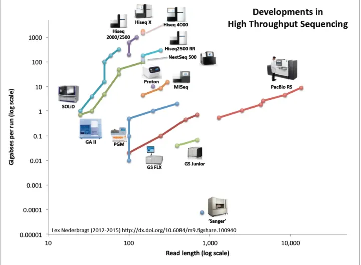
& Syvänen, 2011; Quail et al., 2012). Since the introduction read length and read number are increasing for different technologies (Figure 1).
Figure 1 also shows the appearance of the latest sequencing technology, third generation sequencing, which is based on single molecule sequencing introduced by Pacific Biosciences for
Figure 1. Development of read length and read numbers of different NGS technologies.
The x-axis shows the read length and the y a-axis the number of reads produced. The different colours show the
different NGS technologies. The figure was generated by Lex Nederbragt (Nederbragt, 2014)
Basic concept of IIlumina sequencing technology
DNA is extracted, sheared and ligated to adaptor oligos at both ends of each DNA fragment. The adapters contain linker sequences to enable binding to the surface of a so-called flowcell. The flowcell itself is a glass plate containing complementary oligo adaptor sequences fixated on its surface. Ligated molecules bind randomly to the flowcell. After binding of the fragments, a local amplification (“ bride amplification ”) is initiated by adding non-labelled nucleotides producing high- density clusters of the fragment sequences. After several cycles of amplification, sequencing begins by annealing the sequencing primers. Fluorescence-labelled terminator nucleotides are added and incorporated by DNA polymerase, which interrupt polymerase activity after incorporation of individual nucleotides. A laser scanner is used to excite the flourophores of the nucleotides, which then emit a light pulse, which is recorded as an image of the flowcell. The terminator is then enzymatically cleaved out and the next cycle can begin. The image files are converted into sequence data by “basecalling” software (Metzker, 2010).
The Illumina platform also offers paired-end sequencing, where reads are generated from both ends of the fragments. The number of reads increased over time and now allows sequencing of multiple samples on the same flowcell. To reconstruct from which samples reads were derived from a barcoding system was introduced. Those barcodes are short unique nucleotide sequences (commonly around six nucleotides) added to the adapter of each sample, ensuring that each read can be assigned to its source sample (Bystrykh, 2012; Mir, Neuhaus, Bossert, & Schober, 2013;
Van der Auwera et al., 2002).
Genotyping using NGS genotyping by sequencing (GBS)
NGS allows screening for thousand of markers in one analysis, which allows identifying allelic variation at high resolutions. As described in the previous section, millions of reads are generated containing short genomic information of the sample. To obtain the allelic differences, the reads have to be transformed into a useful representation. Therefore short reads are aligned to a known reference sequence to order the short reads into a physical representation. The reference sequence is a snapshot of single genome. This approach of aligning read towards a reference genome is known as resequencing. After alignment, the consensus sequence is generated from the aligned short reads for each position of the reference sequence. The difference between the consensus sequence and the reference sequence represent the observed genetic variation from the used genotype compared to the reference sequence.
In general, it is possible to assembly the short reads obtain from the sample into a reference
genome and compare the assembled genomes against each other, but this requires a dense
sequencing depth and huge computational time where resequencing is cost-effective and a fast
method. But it has to be noted as well that resequencing will miss segmental duplications and
available by comparing de-novo assemblies of the genotypes. Genotyping by sequencing (GBS) used the concept of resequencing in a high throughput manner by genotyping for hundred of genomes the genotypes at allelic marker position for each genotype in parallel.
There exists currently two main methods for GBS, the first method based on the whole genome sequencing as described in the previous paragraph and genome complex reduction approaches, i.e. RAD-seq (Baird et al., 2008; Davey et al., 2011; Poland & Rife, 2012). Instead of sequencing fragments produced by random fragmentation of the sample DNA, RAD-seq sequences fragments based on restriction enzyme digestion. Fragments selected for sequencing will have well defined sequence pattern reflecting the restriction recognition site of the restriction enzyme. RAD-seq has two advantages as it reduces the complexity of the genome and allows for high coverage rate at the recognition sites, which allows accurate SNP genotyping. The drawback is the reduction of the resolution compared to whole-genome sequencing as only a limited number of markers can be obtained. To increase the resolution imputation can be applied.
Both methods (whole genome sequencing and complex reductions) are using multiplexing which is highly cost efficient, multiplexing a large number of samples results in low amounts of sequencing data for each of the samples. This can complicate the use of these data for genotyping.
Though GBS is generally a simple concept specific details complicate this simplicity including how to handle heterozygous position, what reads are reliably aligned or how to handle genomes which are not diploid? But the benefit of using NGS for genotyping is the flexibility to screen for known and unknown variations. This allows genotyping by assigning the correct allele for each sample without the requirement of any prior knowledge on SNPs and their alleles.
Genotyping based on sparse sequencing data.
For genotyping of recombinants from controlled crosses, first the variants have to be identified describing the differences between the parental lines. For our purpose we used SNPs as variants (markers). To genotype an individual recombinant line high coverage sequencing can be applied, i.e. for Arabidopsis thaliana an average coverage of 10x is sufficiently enough (Figure 2A).
As such sequencing depth can be quite costly (in particular for species with large genomes), low-
fold (sparse) sequencing is a reasonable compromise.
impute missing genotypes different approaches have been developed. Those approaches make use of high levels of linkage in recombinant genomes allowing imputing missing informations.
Figure 2. Observed allele support (y axis) for the two parental alleles P1 (red) and P2 (blue) on a genomic region (x axis, in Mb). A) Deeply sequenced sample allows for screening for CO and to identify the correct genotype at each marker position. B) In contrast, sparsely sequenced individuals make it difficult to identify COs and the correct genotypes for each marker position. To genotype such samples, we have to apply more sophisticated methods.
Imputation methods can be divided into two types of approaches, studies of direct related or unrelated individuals. Imputing missing genotypes in recombinant individuals derived from controlled crossed (typically even with known parental genomes) relies on long haplotypes.
Identifying such haplotype blocks can be used to impute missing genotypes as each marker in one haplotype block is linked to the same parental genotypes. Imputing natural accessions, e.g.
selected in different countries, relies on the ancestral haplotypes segregating in such populations.
Such methods have been well studied in the field of human resequencing and genome-wide association studies (Marchini & Howie, 2010).
Here we present two approaches for imputing genotypes from recombinant genomes: sliding window and Hidden-Markov Model (HMM).
Imputation using a simple sliding window approach
Huang et al., 2009 published a sliding window approach for genotyping 150 RILs from a bi-parental
population derived from a cross of indica and japonica rice lines. The average coverage per
sample was 0.02x. They applied a sliding window of 15 SNPs per window over 1,226,791 SNPs
(3.2 SNPs/kb), counting only informative SNPs labeled by their support for indica or japonica
be calculated given the frequency of observed genotypes in that window. The thresholds for assigning genotypes are dependent on the window size. If the window size has to be modified, e.g.
the window size has to be increased, as the marker density is too low, the expected probabilities have to be changed. Additionally the threshold for identifying heterozygous regions is problematic to estimate, as it has been defined as a high up and down in a short range. In general, the benefits of a sliding window approach includes that it is quite simple to apply and fast, however sliding window approaches have a low resolution as not each marker is individually imputed.
Hidden-Markov Model (HMM)
To increase the genotype resolution (and accuracy), imputation based on HMM was introduced (Andolfatto et al., 2011; Xie et al., 2010).
A HMM is an extended version of a Markov chain. A Markov chain is a statistical model predicting a future event given the knowledge of previous experiences. The Markov chain can be described as a chain of states = { , , , , … , } . Each state is representing an observable event. The probability , , = {1 … } describes the probability of observing an event after observing
, = {1 … } . The set of all possible is known as transition matrix.
A Markov chain of order 1 is a model consisting of a finite set of states = { , , , , … , } and a transition matrix = { } , , = {1 … }, ℎ ∑
, ,= 1 . And for all ∈ the probability of the transition → is determined by
�+= |
�= = { }, where x represents time.
A Hidden-Markov model (HMM) extends the Markov chain, where observation events are not representing the states. The states are hidden and can only be predicted based on the observation. A HMM is defined by an alphabet S, a set of states Q, a matrix � = { } , ∈ , emission probability for every ∈ and ∈ and an initial starting probability for observing a certain state at the beginning.
By combining the transition and emission probabilities a solution space is defined, where all possible combination can be described and each chain of events can be evaluated by their probability. In other words: Let � = � , �
,, … , �
�be a possible path generated by our HMM for a given sequence x = ( , , … ,
�). The probability for , � =
�1∏
�= �� ����+1with �
�+. We need to calculate each possible path and take the path with the highest probability ( �
∗): �
∗=
�
, � . To reduce the computational time the Viterbi algorithm is used (Rabiner, 1989).
In the following chapter we will use HMMs to correct and impute genotypes using sparse sequencing for bi- and multi-parental mapping populations. For the bi-parental section we developed a similar model as proposed by Andolfatto et al. 2011 and Xie et al., 2010. The differences between these appraoches is in the esitmation of transition and emission probabilities and which information is used to construct the sequence of observations for the HMM. Xie et al.
designed a HMM for the genotyping of a RIL mapping population of a cross of rice varieties allowing them to apply expected probabilities for transition and emission probabilities. As for a RIL population only homozygous genotypes are expected. Andolfatto et al. introduced a more general form of the HMM approach primarily designed for a RIL population from flies. They applied a Bayesian approach to calculate the probabilities under the constraint that only one crossing over per chromosome is expected and that the error rate is equal for each individual. We will present an approach predicting the genotypes using a sample-wise error rate and no constraints regarding crossing over rates.
For the multi-parental section we will use a two stage HMM for genotyping homozygous regions first and then assigning the two parental lines to the heterozygous regions in a second step. We will start by introducing a method to genotype bi-parental mapping population as imlemented in the newly developed pipeline TIGER (Trained Individual GenomE Reconstruction).
1. Genotyping by sequencing for bi-parental crosses
This chapter covers genotyping by sequencing for bi-parental crosses. We will start by introducing the method used for genotyping based on the previous introduction chapter. The result section is followed by a description of different projects that used the method. And finally the chapter will be closed by a discussion. The presented methods have been used to investigate whether the absent of RECQ4a could increase the recombination rate in Arabidopsis thaliana (Rowan, Patel, Weigel,
& Schneeberger, 2015). Furthermore two more projects on genotyping a F
2mapping population of Strawberry plants and for genotyping a Sorghum bicolor RIL population.
The methods part will explain how we approach the problem of imputing missing and removing false genotyped information for each given marker position based on NGS data. Imputation and correction is necessary as we are handling sparse sequencing data for each individual, which is challenging. We used a machine learning algorithm based on a HMM to solve this task.
1.1 Method
In this section we present the algorithmic approach for genotyping by sequencing of sparse resequenced data for bi-parental crosses. We called our approach Trained Individual GenomE Reconstruction (TIGER).
1.1.1 Premises for using the TIGER pipeline
Before we can apply TIGER to sequencing data, the data itself has to fulfill certain criteria:
1) The sample data comes from a resequencing project; reads can be aligned towards an existing reference sequence from the same species as the recombinants. It not recommended applying a different reference species as chromosomal rearrangements could generate patterns similar patterns to those introduced by recombination. This would generate false training information for the HMM.
2) The mapping population is generated from two parental lines.
3) A genome-wide set of SNPs differentiating both parents needs to be available. The density of the SNP set defines the resolution of identifying genotype blocks.
4) The crossing scheme for the recombinant population needs to known, as it is used for
genotype predictions .
obtained a list of raw SNPs using SHORE for SNP calling (Ossowski et al., 2008). However, raw SNPs calls typically contain false positive SNPs.
Therefore we applied strict SNP filtering. First SNPs located in mitochondria- and chloroplasts DNA are removed, followed by removing SNPs reporting insertion or deletion (InDels) events, as TIGER does not consider insertion and deletions (InDels) for genotyping (see Discussion). Further SNPs are only considered if they are of high quality (minimum SHORE quality score of 30) and found in uniquely aligned reads. Additionally we remove SNPs which are located in a region where the surrounding genomic sequence is not supported by the reference sequence with high read mapping quality, because this indicates possible rearrangement in the close vicinity, which can complicate SNP calls in particular in low fold sequenced genomes. The remaining SNPs are further filtered for overlap with transposable elements to reduce the impact of possible rearrangements in the genotyping call (Wijnker et al., 2013) and a global read coverage filtering is applied to remove too low or too high coverage region. This setup allows only SNPs with read coverage within two standard deviations of the average genome-wide coverage. Finally, we used the segregation patterns of the SNPs in the F
2population to remove SNPs, which did not show a Mendelian pattern of inheritance to obtain a final set of markers. These filtering steps reduce the genotyping errors that might arise from poor quality markers.
1.1.3 Pre-assignment of genotypes at individual marker positions
Typically recombinant population are large, and sequencing of those requires following multiplex based sequencing protocols. In general the sample DNA is first fragmentised and fragments are selected based on their length and sample-specific adaptors are ligated. This is done for each sample independently; afterwards samples are pooled for sequencing run on a NGS machine (Baird et al., 2008; Mir et al., 2013; Wong, Jin, & Moqtaderi, 2013).
After the reads are de-multiplexed, based on their barcode signature (Craig et al., 2008), the reads of each individual sample are aligned against the reference sequence. Then we record the allele frequency for each parental allele at each SNP marker by counting the number of aligned reads supporting the parental allele. The allele ratio can already be used for genotyping, however, the low amount of reads per marker make these call error prone.
In order to prepare for genotyping with TIGER, the read counts are transformed into three possible
genotype states e.g. homozygous state for parent A or B and the heterozygous state AB (parent A
and B are synonyms for the parental genomes). To model the low sequencing marker situations
additional three states are included AU, BU and UU, where AU or BU represent the uncertainty
about the second chromosome and is applied if less than five reads for that position are recorded
(U for unknown). UU is being reported if no information could be obtained for that SNP position, i.e.
no reads aligned to this marker. The translation of the allele ratio counts into the alphabet of six states is performed as follows:
1) An allele count threshold is used for labeling homozygous states. The homozygous states (AA or BB) will be assigned if at least five reads are supporting only one of the parents at that SNP position.
2) For all other ratios, we calculated the probability of observing the allele counts from a homozygous or heterozygous background using a multinomial distribution. First we calculate the probability of drawing allele counts for either parent A or parent B in a homozygous background (x
1,x
2) (Equation 1). We assume 1% sequencing error. For a heterozygous background (f(a,b)) we consider that the probabilities for each allele would be equal to p=0.5. To determine the genotype we first compare x
1and x
2and take their maximum which is then compared with f(a,b). The last comparison determines if we have a homozygous are heterozygous genotype. If the maximum is greater than f(a,b) then homozygous state (AU or BU) is reported based on which variable was greater (x
1or x
2).
The transformation of the allele frequency counts at each position into our six genotypes simplifies the construction of the HMM as we do not have to model distributions being emitted from our hidden states.
Equation 1. Probability for drawing one of the parental genotypes (x
1or x
2) in the homozygous background and the probabilities to draw them together coming from a heterozygous distribution (f(a,b)).
1.1.4 State model of the HMM implemented in TIGER
The pre-assigned genotypes could already represent the final genotype output, but it contains markers with no genotyping information at all which lowers genotyping resolution. Additional to missing information, wrong genotype calls are still possible even given our strict filtering steps. To predict and correct genotypes we use a HMM approach. The connection between the hidden states reflects their relationships towards each other and the probabilities of a transition. A
x
1= (a + b)!
a!* b! * 0.99
a* 0.01
bx
2= (a + b)!
a!* b! * 0.99
b* 0.01
af (a,b) = (a + b)!
a!* b! * p
a* p
b, p = 0.5
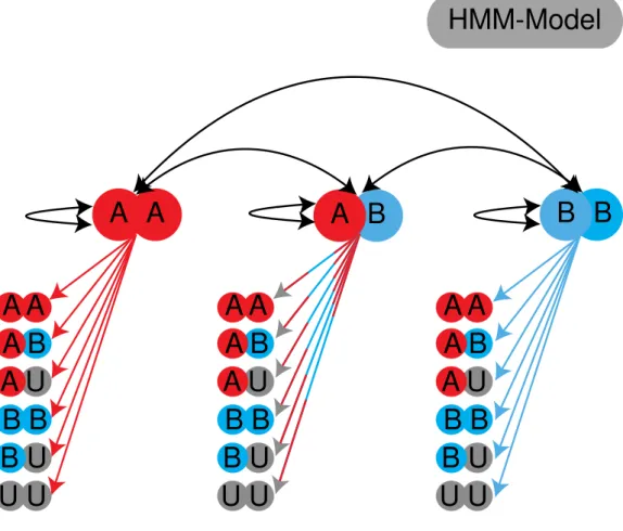
each other, and each hidden node had six emission states, reflecting the alphabet that was assigned as genotypes to each marker (Figure 3).
Figure 3. Schematic of the state model used in TIGER. Red indicates parent A, blue indicates parent B and grey absence of information.
1.1.5 Parameter estimations for the Hidden-Markov Model (HMM)
To finalize our model we need to add the missing transition and emission probabilities. There are different ways to estimate those either by training the model using genotyping data (supervised) or by training on the provided data set (unsupervised) (Rabiner, 1989). TIGER estimates the probabilities for each sample separately without the need for any additional information on error rate, allele bias or similar, besides the inbreeding depth of the sample. In order to get sample- specific HMMs and their probabilities we broadly estimate the genotypes using a simple sliding window. For this we first have to estimate the local allele frequencies from all chromosomes by applying a simple sliding window e.g. of 1,000 adjacent markers. In each of the window the sum of allele ratio per marker is calculated, similar to the already presented sliding window approaches (Xuehui Huang et al., 2009). The size of the sliding window should be chosen based on the filtered marker density and the expected noise level. Therefore a graphical output can be produced to
HMM-Model
A A A B B B
A B A U A A
B B U U B U
A B A U A A
B B U U B U
A B A U A A
B B
U U
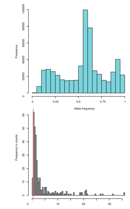
B U
The goal of the sliding window is to reduce the noise ratio to recover the distribution of the allele frequency ratios. This step already assigns genotypes to all marker positions (Xuehui Huang et al., 2009) but this does not allow for a highly accurate resolution of the CO breakpoints. In the ideal case the result of the sliding window reflects the allele frequencies 0, 0.5 or 1 based on the ratio of the parental alleles. However, due to random sampling, sequencing errors, parental allele biases mis-alignment and windows that include regions with different allelic states the distribution is distorted and does not allow for unique assignment of an uniform genotype to each of the windows. The frequencies of the resulting allele ratios from the sliding windows can be plotted as a histogram, which represent the observed allele ratio distribution for that genome. To this observed distribution we fit three beta distributions, representing the expected three different allele frequency distributions representative for the three possible genotypes.
To fit the beta distribution a beta-mixture model with an expectation-maximization (EM) algorithm is applied, which is adapted from (Ji, Wu, Liu, Wang, & Coombes, 2005). After fitting the three beta curves, we label each of the underlying allele frequency under each curve accordingly:
homozygous for parent A, heterozygous or homozygous for parent B. The area under the curves is
limited by 0, 1. We then can apply a supervised learning strategy to obtain the transition and
emission probabilities by combining the allele frequencies and the previously genotyped labels
based on the beta-mixture model thresholds (Figure 4).
1.1.5 Increasing the CO resolution by incorporating removed low quality markers
Tiger is genotyping a set of high quality filtered SNP markers. To increase the resolution for each sample we integrate previously removed markers into regions near the predicted CO breakpoints by a simple gap filling approach. We include from both sides of the breakpoint markers supporting the predicted genotype until the recombination breakpoint. The filling allows one marker not supporting the predicted genotype if their neighboring marker supports again the predicted genotype (Figure 5).
Figure 5. Closing of the predicted CO position by incorporating removed markers (black). The genotype is used to estimate a possible CO by using the last correct genotyped marker.
Parent 1 Parent 2 heterozygous
Figure 6. Workflow of TIGER
A) SNP markers for both parental genotypes have to be identified. Using high-density coverage data reveals
SNPs. For example, in red A. thaliana Col-0 and in blue Ws-2, SNPs in bold. B) Realignment of short read data of
a sparse sequenced individual. Short strings represent reads and SNPs in bold, colouring indicated which
genotype the reads supports. At each SNP position the number of read counts for each genotype is counted per
position and applied to the HMM parameter estimator for estimation of the transition and emission probabilities
for the HMM. C) The read counts of each SNP position for each genotype is called and transformed into one of
1.1.6 In-silico validation of TIGER
To validate our pipeline we simulated three different F
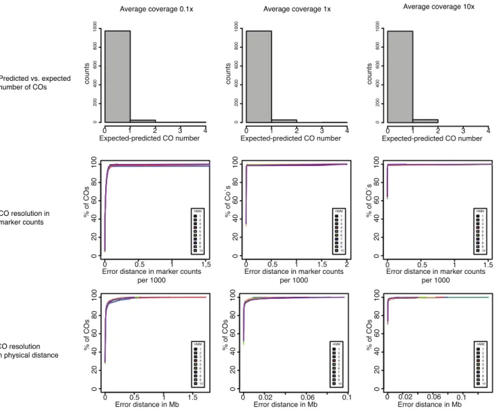
2A. thaliana mapping populations, each containing 1,000 samples, with three different read coverage rates (0.1x, 1x and 10x) using the Pop-seq tool (James et al., 2013) with the default recombination landscape from Salome et al 2011. We used a simulated error rate of 1-3% and genotypes were generated at 261,795 high- quality SNP markers. The 1,000 samples were randomly distributed into 10 separate batches and for each batch we determined the number of predicted recombination events, the breakpoint resolution, and the types and genomic positions of errors produced by applying TIGER (Figure 7).
We combined the results from 10 bins for each of the simulated coverage rates independently. We compared the difference between the predicted COs and the numbers of expected COs based on the simulated data. The difference between expectation and prediction was always positive, irrespective of coverage rate. This indicates a tendency of TIGER to underestimate the number of COs. As expected by increasing the coverage rate the percentage of COs that were not predicted decreased from 2.5% for the lowest coverage (0.1x) to 0.7% for the highest coverage (10x) (Figure 7).
To estimate the resolution of the predicted CO positions, we used the physical distance as well as the number of markers between the predicted and expected CO position. We found that the resolution improves with increased coverage. More than 90% of the COs were predicted on average within a distance of 2 kb from the expected CO position. The average number of markers between predicted and simulated CO for 0.1x coverage was 7, for 1x 1 and 10x 0. The average resolution at 0.1x was 1,986 bp (Table 1).
Table 1 Simulation results
The difference between predicted and simulated CO positions were used for estimating the quality of the prediction based on simulated data
Average coverage CO identified Median resolution (bp)
≤ 90% ≤ 98% ≤ 90% ≤ 98%
Marker numbers Physical Distance (kb)
0.1x 38 79 27 222 1985.5
1x 4 10 4 94 937.75
10x 2 3 1 30 0
Figure 7. Validation by simulation
We simulated three different coverage rates 0.1x, 1x and 10x (columns). The first row describes the difference between predicted and simulated COs regardless of their location. The middle row shows the difference between predicted and simulated COs in marker counts (x-axis per 1,000 markers and y-axis the percentage of COs located in that interval). The last row shows the same information as the middle row but measured in physical distance (x-axis in Mb).
1.1.7 Errors detected during in-silico validation
Analyzing how many errors and what kind of errors are produced while reconstructing the simulated genome data allowed us to analyze these types of errors.
The most dominant error (89% of all errors) was mis-predicting heterozygous genotypes as
homozygous but simulated heterozygous or the predicted homozygous genotype) was 0.1%
regardless of the coverage (Figure 8).
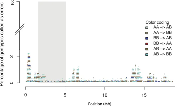
Regions adjacent to the centromere exhibited a high marker diversity, which dropped off at the border of the centromere including repeats, wrong and missing reference sequence information that is the most likely reason for this type of error (Figure 8). To exclude a bias for predicting only for a certain parental homozygous genotype wrong, we analyzed the false homozygous error rate per parental allele. False homozygote regions represented either 42% or 47% for either one of the parental homozygous, indicating that this type of error was not biased towards one of the two parental genotypes.
Figure 8. The frequency of different types of genotyping errors produced by TIGER using simulated data.
An example of an error profile for Chromosome 4 is shown (results were similar for the other four
chromosomes). The grey box indicates the location of the centromere. The error frequencies were obtained
from genotypes predicted from read data from 1,000 simulated recombinant individuals. X-axis genomic scale in
Mb and y-axis the percentage of wrong predicted genotypes.
1.2 RESULTS
In this section we will describe the application of TIGER applied on real data. We present three different projects where TIGER was used for genotyping individuals from mapping population with sparse sequencing data. Each project covers a different taxa and a different motivation for genotyping individuals from a mapping population.
1.2.1 Applying TIGER on individuals of a mapping population of A. thaliana 1.2.1.1 Introduction
In yeast and in humans exists a homologous protein of A. thaliana RECQ4a, SGS1 (yeast) and BLM (human). These proteins are involved in resolving CO intermediates (Knoll & Puchta, 2011). It has been shown that RECQ4a can partially restore the meiotic defects in yeast sgs1 mutants (Bagherieh-Najjar, de Vries, Hille, & Dijkwel, 2005). A defect in RECQ4a in somatic cells of A.
thaliana increased the CO rate (two to seven-fold) (Hartung, Suer, & Puchta, 2007). Higgins et al.
2011 found out that the RECQ4a is localized at the telomere regions and along the chromosome axes, partially interacting with CO proteins but also found evidence that RECQ4a is actually resolving telomeric bridges (Higgins, Ferdous, Osman, & Franklin, 2011). Therefore we have here conflicting observations regarding the involvement of RECQ4a during meiosis in resolving CO intermediates. To investigate this we (Rowan et al., 2015) developed two mapping population, a wild type and a recq4a (mutant) population based on the background of the parental genotypes Col-0 and Ws-2 and mutants with the same background, respectively. Each population consists of 196 individuals. Both populations were sparsely sequenced and genotyped using TIGER.
First we have to generate markers. SNPs were generated by analysing Ws-2 (25x) against the Col-0 reference. From the high-coverage data we found 840,611 SNPs between Ws-2 and Col-0 (TAIR10). After removing the SNPs located in the mitochondria and chloroplasts genomes and those close to indel polymorphisms, 745,273 SNPs remained. An additional 238,111 SNPs were removed after considering only high quality SNPs and those supported only by uniquely aligned reads. We further decreased the marker number to 302,082 after applying filtering for homozygous regions, transposons and coverage filtering. Finally we removed 40,287 SNPs that did not show a Mendelian pattern of inheritance in our F
2population to obtain a final set of 261,795 markers.
The F individuals were sequenced on an Illumina GAIIx analyzer in one flow cell lane using 2 x
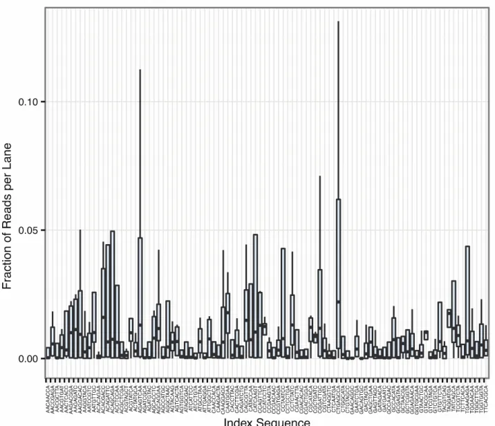
Figure 9. Sequencing statistics for the barcodes used to produce the sequencing data.
The x-axis represents the barcode sequence and the y-axis shows the fraction of reads per lane.
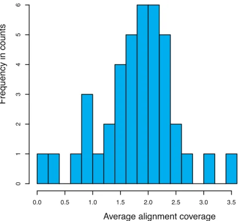
1.2.1.2 Reconstructions of wild type and recq4a F2 sample genomes
An average genome-wide coverage threshold of 0.025x was used to remove samples with too little
sequencing data as the accuracy of correct CO breakpoint prediction was strongly reduced at such
coverage rates. After filtering, 216 individuals could be reconstructed (110 from the wt population
and 106 from the recq4a population), overall representing an average coverage of 0.63x and a
median coverage of 0.37x. From our simulation studies we already observed several types of
errors (Figure 8) but we encountered a new additional type of a possible errors, where small
genotype blocks were embedded within larger blocks of a different genotype. We termed these
regions “islands” , which could either be false positive or real double recombination events (Figure
10).
Figure 10. Illustration of an island structure
Illustration of read support (y-axis) for either one of the parental allele (red or blue) for F2 sample for one of the chromosomes (x-axis). The purple box shows a genotyping island showing a homozygous genotype for one of the parental allele
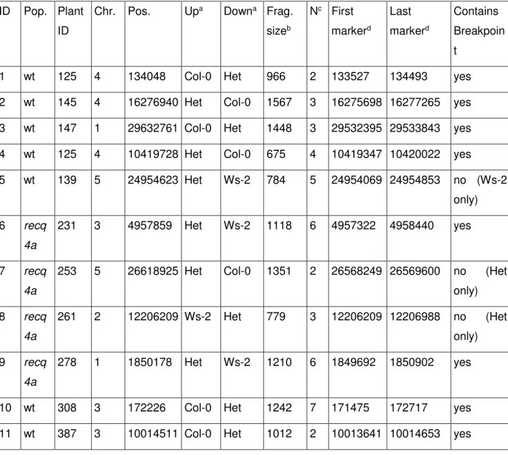
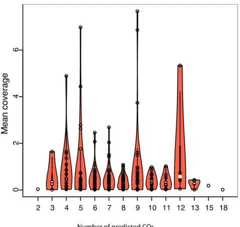
We used the island length distribution for filtering for wrong signals. From 67 islands, 7 were less than 400-kb long and were removed (Figure 11). The remaining 60 islands were categorized as double COs. After the error correction step, the final genome reconstructions can be used for further analyses, i.e. whether the observed CO rate is dependent on the coverage rate. We observed that the CO predictions were hardly affected (Figure 12). After introducing removed markers next to the predicted breakpoint sites, we could resolve the majority of COs to an interval of two kb or less (Figure 13). For validation eleven CO breakpoints were randomly selected for PCR and Sanger sequencing. Eight of the eleven breakpoints were in the predicted two-kb intervals (Table 2).
The observed breakpoint resolution of our experimental F
2populations closely matched that of the
simulated populations at 0.1x coverage. Given the median coverage rate of 0.3x this indicates that
the simulation was quite fitting and therefore the expected error rate based on the simulation data
should be in the same region for our experimental set. Finally, we verified that the overall
frequency of Col-0, Ws-2 and heterozygous genotypes in both populations was consistent with the
expected pattern of inheritance (
Table 3) before comparing the CO patterns between both populations.
Table 2 CO An evaluation of CO break point predictions using TIGER and PCR comparison
a
Genotypes predicted up or downstream of the CO point
b
Size of the PCR fragment amplified
c
number of markers covered by Sanger sequencing reads
d