16 Maverick: Experimentally Testing a Conjecture of the Antitrust Authorities

Conjecture of the Antitrust Authorities

Abstract: Antitrust authorities all over the world are keen on the presence of a partic- ularly aggressive competitor, a “ maverick ” . Yet there is a lack of theoretical justifica- tion. One plausible determinant of acting as a maverick is behavioral: the maverick derives utility from acting competitively. We test this conjecture in the lab. In a pre- test, we classify participants by their social value orientation. Individuals who are ri- valistic in an allocation task indeed bid more aggressively in a laboratory oligopoly market. This disciplines incumbents. We conclude that the existence of rivalistic atti- tudes may justify antitrust policies that protect mavericks.

16.1 Introduction

One man ’ s meat is another man ’ s poison, as they say. Antitrust is a field of applica- tion. For those forming a cartel, or coordinating tacitly, collusion is a dilemma.

Individually, each is best off if the others are faithful cartelists, while this one firm undercuts price, or exceeds the quota for that matter. However, if cartelists succeed to coordinate, this has negative external consequences for consumers. Antitrust au- thorities are therefore pleased to learn that one supplier in a market is particularly aggressive. The US Horizontal Merger Guidelines have coined the graphic term

“ maverick ” for such firms. The Guidelines describe such firms as “ firms that are un- usually disruptive and competitive influences in the market ” .

The European Horizontal Merger Guidelines express the same concern.

Christoph Engel,Max Planck Institute for Research on Collective Action, Bonn Axel Ockenfels,Department of Economics, University of Cologne

Notes:Helpful comments by Uwe Cantner, Dominik Grafenhofer, Marco Kleine, Vincenz Frey and several anonymous referees, and discussion at the Rotterdam Department of Economics, are gratefully acknow- ledged. Ockenfels gratefully acknowledges financial support from the Deutsche Forschungsgemeinschaft (DFG, German Research Foundation) through the Research Unit“Design & Behavior”(FOR 1371) and under Germany’s Excellence Strategy (EXC 2126/1–390838866), as well as from the European Research Council (ERC) under the European Union’s Horizon 2020 research and innovation program (GA No 741409). This paper reflects only the authors’view and the funding agencies are not responsible for any use that may be made of the information it contains.

1 57 FR 41552, sec. 2.12 at note 19; the concern is upheld in the new, 2010, version of the guidelines, http://www.justice.gov/atr/public/guidelines/hmg-2010.pdf, sec. 2.1.5 and sec 7.1

2 OJ 2004 C 31/5, no. 20, no. 42.

Open Access. © 2020 Christoph Engel and Axel Ockenfels, published by De Gruyter. This work is licensed under a Creative Commons Attribution-NonCommercial-NoDerivatives 4.0 International License.

https://doi.org/10.1515/9783110647495-016

In the next section, we review the case law and the (rather small) economic lit- erature on maverick behavior. In this paper, we focus on one potential source of aggressive market behavior that has gotten short shrift. Market participants might bid aggressively because they hold particularly competitive preferences. They might derive utility from getting a higher payoff than their peers. In this sense, our study looks at macro-level implications of individual social preferences and thus builds on most of the literature, which asserts that such preferences exist in the field (see refer- ences in Ockenfels et al. 2015).

A preference-based explanation for aggressive market behavior, and its effect on the behavior of other market participants, would be hard to study in the field, if not impossible, though. This is why our study is conducted in a controlled laboratory en- vironment, despite the inevitable wedge between our object of interest (the behavior of firms in a product market) and our object of study (the behavior of students in a laboratory market); we further discuss external validity in the concluding section.

Social preferences are assumed to be personality traits. Personality traits cannot be induced on the spot, but they can be measured. We proceed in two steps. In a first experiment, we classify participants by their social value orientation (Liebrand and McClintock 1988). We select those participants with the most rivalistic social value orientation to be entrants in the second, main experiment. For 10 periods entrants observe how two participants randomly selected from a pool with less extreme social value orientation choose quantities in a duopoly market. We investigate whether the behavior of incumbents, and market outcomes, differ according to the social value orientation of the entrant.

Our main hypothesis is supported with a proviso. Conditional on local market conditions, firms perform worse on average, and consumer welfare increases, if the market entrant is classified as rivalistic. Yet local conditions matter. In particular, rivalistic entrants do not make the market more competitive if competition was al- ready fierce in the first place.

The remainder of the paper is organized as follows: section 2 defines our contribu- tion to the legal and economic literature. Section 3 presents the design of the experi- ment and our hypotheses. Section 4 reports the results from the main experiment.

Section 5 concludes with discussion.

16.2 Mavericks in practice and in economics

The concept of mavericks has led to a rather rich case law. In United States vs.

ALCOA, government sued ALCOA for divestiture of the acquisition of Rome Cable Corporation. The Supreme Court held that the acquisition constituted monopoliza- tion, on the argument that “ Rome was an aggressive competitor ” (377 U.S. 271 [281]

(1964)). Likewise, in Mahle GmbH, the Federal Trade Commission forced Mahle

GmbH to divest Metal Leve ’ s United States piston business on the argument that, before the merger, Metal Leve was “ an aggressive and innovative competitor ” (62 Fed.Reg. 10,566 [10,567] (1997)). The Antitrust Division of the Department of Justice opposed the acquisition by Alcan Aluminium Corp. of Pechiney Rolled Products, LLC, since this would “ remove a low cost, aggressive, and disruptive competitor in the North American brazing sheet market ” (Case No. 1:03CV02012, para. 21 (2003)).

Likewise, the Federal Trade Commission opposed the proposed merger of Staples, Inc.

with Office Depot, Inc., on the argument that the merger would eliminate a “ particularly aggressive competitor in a highly concentrated market ” (Case No. 1:97CV00701, sec. IV A 2 (1997)). These decision are echoed by legal doctrine (Baker 2002; Kolasky 2002).

The European antitrust authorities have taken similar decisions. The European Commission cleared the merger of T-Mobile Austria with tele.ring only after the parties committed to selling major assets of tele.ring to an independent competitor. This under- taking was requested, although the new merged unit would not be the largest supplier in the Austrian market for the provision of mobile communication services to end cus- tomers since, before the merger, “ for the last three years, tele.ring has played by far the most active role on the market in practising successfully a price aggressive strategy ” (case M.3916, O.J. L 88/2007, 44, para. 10). Likewise the Commission cleared the merger of Linde with BOC only after both firms committed to selling a number of major supply contracts concerning helium. This removed the Commission ’ s original concern that, otherwise, Linde would stop “ compet[ing] aggressively to expand its position on this market ” (case M.4141, IP/06/737 (2006)). An interesting case is Euler Hermes/OEKB.

Through the merger, the new unit reaches a share between 45 and 55% on the Austrian market for delcredere insurance. The Commission nonetheless does not see reason for concern, one counter argument being that an independent new entrant Atradius “ has assumed the role of a maverick by its aggressive pricing policy and its increase of sales ” (case M.4990, para. 29, 2008).

There is also empirical data suggesting that mavericks exist, and that they can substantially change market behavior. One study compares prices for retail gas in the otherwise comparable metropolitan areas of Ottawa and Vancouver. In both re- gions, tacit collusion would be equally feasible. Yet data from Internet price data collection sites show that, in the Ottawa region, prices are much more dispersed and volatile. This market outcome can be traced back to the presence of a maverick (Eckert and West 2004a, b). Maverick behavior has also been identified in the Australian mortgage market (Breunig and Menezes 2008). Another illustration is be- havior in the Dutch spectrum auction in 2000 (Van Damme 2003, see also Klemperer 2004). There were five incumbents and five licenses for sale, but several potential en- trants. As Van Damme (2003) emphasized, the Dutch telecom regulator “ hinted at

3 http://www.justice.gov/atr/cases/f201300/201303.pdf.

4 http://ec.europa.eu/competition/mergers/cases/decisions/m4990_20080305_20310_de.pdf.

the desirability to favor newcomers to the market in the auction ” , and that “ there are several reasons why a new entrant might be a more aggressive player on the market ” . However, all but one potential entrant (Versatel) actually partnered with an incum- bent bidder, removing them from the auction market. One of the incumbents (Telfort) later, during the auction, accused Versatel of particularly aggressive bidding behav- iors. As Van Damme (2003:285) reports: “ Telfort claims that Versatel is bidding only to raise its rivals ’ costs or to get concessions from them. ” (Cramton and Ockenfels 2017 make a related point in the context of Germany ’ s 4G auction.)

That said, there is a gap between the practice of dealing with mavericks in com- petition policy and the economics of mavericks in theory. Simple economic explan- ations of why some firms are more competitive than others would include that mavericks have lower costs, are incentivized by sales volumes, or control more ca- pacities than their competitors. All this would imply that mavericks have a rather large market share. Yet, as Breunig and Menezes (2008) pointed out, competition authorities often stress that mavericks are, in fact, likely to be small firms (which seems to make it more plausible that personality traits of managers play a role in the phenomenon of mavericks). This might follow from pronounced switching cost, which forces entrants to be particularly aggressive (Farrell and Klemperer 2007), from more pronounced discounting of future earnings by firms in financial distress (Busse 2002), or from the fact that fixed cost is high in the industry (Scherer and Ross 1990). Yet another, underexplored source of aggressive behavior is behavioral.

Some, but not all, decision makers like to be ahead, and dislike being behind. It is this source we are studying in this paper.

Our approach resonates with the New Zealand Merger Guidelines. In their sec- tion 7.2, the guidelines explicitly list “ features associated with a maverick ” . Most features relate to a behavioral tendency to disrupt coordination and similar phe- nomena, including the first feature ( “ a history of aggressive, independent pricing behavior ” ) and the last feature ( “ a history of independent behavior generally ” ).

In the same spirit, Kwoka (1989) adds a firm specific degree of conjectural variation in quantity choices to a fully symmetric Cournot model.

In the US the focus on “ maverick ” firms has come under attack. Antitrust au- thorities have been urged to put less weight on the issue, mostly because there is so little theoretical foundation in economics.

However, in our view, the normative de- bate of the role of mavericks would benefit if it were to adopt a more adequate con- cept of competitive behavior. Individuals strongly differ with respect to social behavior, including their competitiveness, willingness to cooperate or collude, and

5 http://www.comcom.govt.nz/assets/Imported-from-old-site/BusinessCompetitio n/

MergersAcquisitions/ClearanceProcessGuidelines/ContentFiles/Documents/Mergers-and- AcquisitionsGuidelines-2003.pdf, accessed 1 January 2014.

6Personal communication by the chief economist of the German Cartel Authority, Konrad Ost.

ability to coordinate. In fact, individual heterogeneity in social and economic inter- action is one of the most robust insights from behavioral economics and psychology (e.g. Camerer 2003). Thus, heterogeneity of social preferences may be one important missing link between antitrust practice and economic theory when it comes to un- derstanding the presence of mavericks.

There are many ways of modeling social preferences (for a survey see Cooper and Kagel 2016). Many models include a concern about relative, not only absolute payoff. Such models describe, for instance, inequity averse players (Fehr and Schmidt 1999; Bolton and Ockenfels 2000) or rivalistic players, who are willing to trade some absolute payoff against a sufficiently higher relative payoff (Fouraker and Siegel 1963: chapter 9; Bolton 1991; Frank 1984; Bazerman, Loewenstein, and White 1992; Messick and Thorngate 1967). These models resonate with an extended literature in social psychology on the “ desire to win ” (for a summary see Malhotra 2010). There is pronounced heterogeneity with respect to this desire (De Dreu and Boles 1998; Van Lange et al. 1997). The desire to win can lead to bidding more in an auction than the item is worth (Ku, Malhotra, and Murnighan 2005) and to engage in costly litigation rather than settling a case (Malhotra, Ku, and Murnighan 2008).

Rivalistic behavior is also sometimes characterized as status seeking (Frank 1985; Clark, Frijters, and Shields 2008) and backed by solid experimental evidence (Ball and Eckel 1998; Huberman, Loch, and Önçüler 2004; Charness, Masclet, and Villeval 2013) and evidence from the field (Solnick and Hemenway 1998; Ferrer-i- Carbonell 2005; Luttmer 2005; Boes, Staub, and Winkelmann 2010). The concept of status seeking has explicitly been extended to market behavior (Sobel 2009), en- trepreneurial risk-taking (Clemens 2006) and managing a firm (Auriol and Renault 2008). Status seeking has been shown to affect behavior in experimental markets (Ball et al. 2001) and experimental supply chains (Loch and Wu 2008). In the field, status plays a strong role in motivating managers (Ockenfels, Sliwka, and Werner 2014; Grund and Martin 2017).

The only experimental study of “ maverick ” behavior we are aware of has been conducted by Li and Plott (2009). The paper studies which interventions can break tacit collusion in a laboratory market with 8 participants who hold exogenously given, different valuations for 8 items. The first part of their experiment continues until the group colludes perfectly. One of the interventions, which the authors re- late to the anti-trust concept of a maverick, consists of confidentially changing the valuations of 2 items for the duration of 2 periods. As desired, participants with higher valuations, who have been induced to bid more aggressively, start bidding for the item in question. Some other participants retaliate, which leads to a price

7Of course, other areas of industrial organization have already been substantially influenced by behavioral research; see, e.g., Engel (2007) for the insights from experimental economics for the determinants of tacit collusion.

war. Yet after a while, collusion is again established (Li and Plott 2009: 444). Our approach complements their study in various important ways. We mention two points here. First, we study the effects of aggressive quantity choices resulting from personality. That is, our study does not induce aggressive behavior by confidentially changing monetary incentives, but rather focuses on the potential of naturally oc- curring heterogeneity in social motivation to capture maverick behavior. Indeed, because in our context all payoff functions and market conditions are identical and common knowledge across subjects, heterogeneous individual traits are the only possible cause for treatment effects in our experiment. Second, we investigate the effect of “ maverick ” behavior in markets that, endogenously, have produced differ- ent degrees of competition. As we will see, our variables of interest matter: market outcomes can be related to natural psychological traits of traders, and the impact of maverick behavior interacts with idiosyncratically evolved market competitiveness.

Our paper also makes a contribution to the experimental literature on social di- lemmas. To the best of our knowledge, no experiment has tried to explain outcomes in oligopoly markets with the social preferences of participants (cf. the theory paper by İ ri ş and Santos-Pinto 2014). This is surprising given competition can be modelled as a dilemma, and choices in dilemma games are routinely rationalized with the social preferences of participants (for a survey see Chaudhuri 2011). We do not only derive hypotheses from participants ’ social preferences, but even build our treat- ment manipulation on randomly composing markets conditional on participants ’ social preferences.

16.3 Design of the experiment and hypotheses

In order to test the effect of heterogeneous preferences on competition we first clas- sify participants according to their social value orientation in a pre-test, using the standard procedure introduced by Liebrand and McClintock (1988). This test has participants repeatedly choose between two different allocations of a sum to be dis- tributed between an anonymous partner and themselves. They are, for instance, asked whether they prefer 354 units for themselves and an anonymous counterpart over 397 units for themselves and 304 units for the counterpart. Aggregating over all 32 incentivized choices, for each individual one defines a score, which is custom- arily called the “ ringdegree ” since the measure can be represented on a circle.

Participants with a score of 0 only care about their own payoff. Participants with a

positive score are willing to give up some payoff for themselves for the sake of giving

their anonymous partner a higher payoff. Such participants are averse against advan-

tageous inequity, consistent with Fehr and Schmidt (1999), Bolton and Ockenfels

(2000). We are particularly interested in participants with a negative score. They are

willing to give up some payoff for themselves in the interest of increasing the payoff

difference between themselves and their partner. These participants are rivalistic.

They hold a positive willingness to pay for improving their status.

In the main experiment, we form fixed markets of three suppliers to interact in a fully symmetric Cournot market over 20 rounds. In the first 10 rounds, only two suppliers, the incumbents, are active. Every round, the passive supplier, the en- trant, is informed about price and total quantity. This participant only enters the market in round 11. This procedure allows the entrant to observe the market before entering, which seems reasonable for any potential entrant. The social value orien- tation of the entrant is our treatment variable. We have rivalistic entrants, selfish entrants, and entrants who are averse against advantageous inequity. This design reflects the fact that social value orientation, as a personality trait, is not open to ad hoc manipulation. The trait can only be measured, and participants can be matched by the trait. While we are not aware of experiments that have used this approach for social value orientation, it is, for instance, common if one uses gender, age or race as treatment variables (for references in dictator game experiments see, for ex- ample, Engel 2011).

We emphasize that, with the design of the experiment, we do not identify the effect of the presence or absence of a maverick on competition. What we measure is the effect of a change in the structure of the market through the market entry of a maverick. We are thus testing a dynamic, not a static effect (on this distinction see Engel 2016), akin to the distinction between stocks and flows. We have chosen this research question for reasons of external validity. Antitrust, and merger control in particular, have been primarily interested in preserving the competition enhance- ment resulting from such market entry.

The social value orientation test is run a couple of days before the market ex- periment. Participants are invited on the understanding that a second experiment is to follow, but are not informed about the nature of the second experiment. To make matching in the main experiment possible, but preserve anonymity, we use the fol- lowing procedure: at the end of the pre-test, participants themselves generate an identification code. Participants write this code on a card, put this card into an en- velope, seal the envelope and write their name on it. The closed envelopes go to the lab manager. The manager opens them and writes a list that matches names and codes. The experimenter prepares a list with groups to be invited for the main ex- periment. In this list, participants are only identified by their code. The lab manager does not learn any choices participants have made, neither in the pre-test nor, later, in the main experiment. The lab manager only knows who shall be invited for which session. The experimenter never sees the list that matches codes and names.

At the outset of the main experiment, participants identify themselves on the com- puter screen by their code. The program checks whether the invited participants are present.

Participants are completely informed about this procedure. They also know

that the experiment has two parts, and may therefore infer that information from

the pre-test is used for inviting participants to one of the sessions of the main experi- ment. Yet participants neither know the nature of the main experiment, nor which information is used for matching (we run a battery of further personality tests the re- sults of which are of no relevance for the main experiment; their only purpose is mak- ing it difficult for participants to infer which personality trait is used for matching).

In particular, subjects are neither informed about behavior in the first experiment nor about social value scores of other participants; in the field, too, other firms usually only observe their competitors ’ behavior, not their preferences or decision making process.

In the main experiment, participants interact in fixed groups of three. The main experiment has two parts.

At the outset, participants only receive instructions for the first part. They are informed that more parts are to follow, and that new instruc- tions will be distributed for the continuation. The first part of the main experiment has 10 rounds. In this part of the experiment, two incumbents of each group have the active role. The entrant has the passive role. Incumbents are not told that the third participant will later enter the market. This design feature is meant to capture the situation when maverick behavior is most important for antitrust: an outsider observes whether aggressive market behavior is likely to be profitable. (We note, however, that being worried about entry could have led to stronger competition and thus reduce the effect of a maverick entrant.) Incumbents compete in a Cournot market where the profit of incumbent i in period t is given by (16.1).

π

= 100 − q

− q

q

(16 : 1)

We thus assume demand to be linear and normalize cost to zero. After each period, incumbents learn the resulting price and their individual profit. Entrants learn total quantity supplied and the price. After the end of period 10 there is a (surprise) re- start of the market. Now entrants become active as well, so that the profit function changes to (16.2).

π

= 100 − q

− q

− q

q

(16 : 2)

The second part of the experiment also lasts 10 periods.

8 In the pre-test, we had the following sequence of tests: social value orientation; risk preferences (Holt/Laury); belief elicitation on 4 problems from the test for social value orientation; Big5 person- ality inventory (short 10 item version); 4 unincentivized questions about trust taken from the German socio-economic panel; basic demographic information.

9Plus a third part meant to test a theoretical prediction that buyouts of the entrant will not occur, which has been confirmed in our data. However, because this is only of secondary importance for our results, we decided to drop this part altogether. We refer interested readers to the working paper version of this article for more details.

Based on the results of the pre-test, three groups of participants are selected to have the entrant role in the main experiment: Those 9 participants with the most negative social value orientation score have the entrant role in the Negative treat- ment. These participants are rivalistic. We form two different comparison groups: 11 participants with a social value orientation score of zero have the entrant role in the Zero treatment. These participants are selfish. Those 11 participants with the highest positive social value orientation score have the entrant role in the Positive treat- ment. The remaining participants are randomly assigned to have the incumbent role in either treatment. Three of them have a mildly negative social value orienta- tion score. 16 of them are selfish. 40 have a mildly positive social value orientation score.

We have 9 groups (27 participants) in the Negative treatment, and 11 groups (33 participants) in the remaining two treatments. Participants are invited using the software ORSEE (Greiner 2004). 52% of participants are female. Average age is 25.45 years.

Participants, most of whom are students, hold various majors. The experi- ment is programmed using the software zTree (Fischbacher 2007). It is run in the Bonn EconLab. In the pre-test, participants on average earn 13.20 € (16.05$ on the days of the experiment). In the main experiment, they on average earn 9.36 € .

We can straightforwardly compute our null hypothesis under the standard as- sumption that all suppliers maximize their individual payoffs. There is a unique subgame-perfect equilibrium strategy for each phase of the experiment,

condi- tional on the number of suppliers in the market, which is given by q

=

, where n is the number of suppliers. Plugging in the respective market size, we get our null hypothesis

H0:Participants’social preferences for competitiveness do not affect market outcomes; only market size matters.

For our alternative hypothesis, assume that there is some heterogeneity of preferences.

In particular, assume that the entrant is a maverick, competing more aggressively than

10The fact that three participants with a negative social value orientation score are incumbents results from a mistake of the lab manager. Since the lab manager did not know their social value orientation scores, these participants were randomly assigned to one of the groups. For five incum- bents we do not know the social value orientation score. These subjects replaced invited partici- pants who did not show up.

11 From the five replacement subjects, we do not have demographic information since the demo- graphic questionnaire was part of the first experimental battery.

12 The tasks participants face in both parts of the experiment are unrelated, so that the difference in earnings across parts is not meaningful.

13 This is because each base game has a unique equilibrium. In fact, if at the beginning of the first phase, subjects had common knowledge about all aspects of the subsequent phase of the experi- ment, the subgame perfect equilibrium of the whole game could be computed, would also be unique and correspond to the equilibrium in each phase of the experiment.

standard theory would predict. Specifically, assume that the entrant not only cares about absolute profit but also about earning more than the competitors, and that this is common knowledge.

Then, like commitment power favoring the Stackelberg leader, the rivalistic supplier sells a larger quantity than in a standard analysis of the Cournot market, and the incumbents – if only interested in own gains – sell a smaller quantity. Total quantity and thereby consumer welfare is larger than if all suppliers hold standard preferences.

This leads to

H1:If the entrant is rivalistic, she sells higher quantities and the market outcome is more competitive.

We mention that we can derive the same hypothesis if we allow incumbents to be rivalistic, too, as long as they are less rivalistic than the entrant (see Appendix I).

16.4 Experiment results

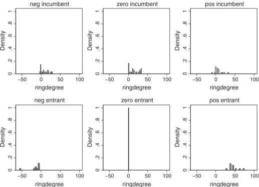
Figure 16.1 informs about the distribution of social value orientation in our sample.

We have 12 (13.64%) rivalistic, 27 (30.68%) selfish, and 49 (55.68%) participants with a more or less pronounced positive social value orientation.

Figure 16.1 also shows our matching. Participants at the lower end of the distribution are entrants in the Negative treatment. These are the subjects with the supposedly most competi- tive behavior in oligopoly markets, and they are thus the focus of our study on the impact of mavericks. Participants at the upper end of the distribution are entrants in the Positive treatment. 11 participants with a social value orientation score of zero are entrants in the Zero treatment. The remaining participants are randomly

14 This is a common assumption not only in large parts of the social preferences literature, but also in the economics literature that does not address social preferences. The assumption simplifies theoretical derivations, although it seems incorrect in most applications. However, in our setting any rivalistic motivation leads to more aggressive bidding, regardless of the extent to which com- petitors are (believed to be) rivalistic. In this sense, the general insight that rivalry leads to larger quantities is robust.

15 We focus onconsumerwelfare for two reasons. Enhancing consumer welfare is the primary stated goal of antitrust policy (Crandall and Winston 2003). Moreover we model mavericks as agents holding social preferences, so that the definition of supply side welfare is not obvious. By focusing on the opposite market side, we are able to bracket this debate in normative economic theory.

16Social value orientation scores range from–56.23 (strongly rivalistic) to 74.55 (strongly averse to advantageous inequity). If a participant chooses the allocation that gives her a higher payoff on all 32 problems, her score is 0. A participant with a score of 45 always chooses the equal split. A participant with a score of 90 is perfectly altruistic. A participant with a score of–45 is willing to give up 1 unit of her absolute profit to increase the payoff gap between herself an her random part- ner by 1 unit. For the procedure for aggregating the 32 choices see Liebrand and McClintock (1988).

assigned to being incumbents in either treatment. To make sure that the 16 selfish incumbents are equally distributed across treatments, randomization is separate for participants with a social value orientation score of 0, and for the remaining incumbents.

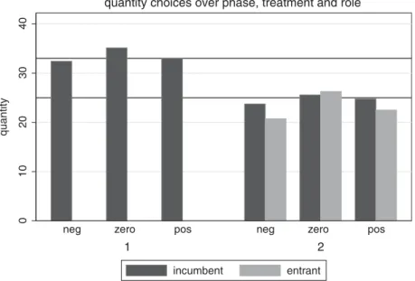
As Figure 16.2 shows, overall quantity choices are fairly close to the standard Cournot predictions. In duopoly markets, average quantity is close to 33. In triopoly markets, it is close to 25. We thus provisionally support our null hypothesis H

. Looking at average quantities only, social value orientation is not a plausible candi- date for identifying maverick behavior. As suggested by Figure 16.2 and Table 16.1, if we work with averages, we do not find treatment effects, neither non-parametrically nor parametrically.

This also holds if we confine the analysis to the last period before and the first pe- riod after entry. Actually, descriptively in the Negative and in the Positive treatments, entrants on average even sell less than incumbents and consequently make a lower profit.

0.2.4.6.81Density

−50 0 50 100

ringdegree neg incumbent

0.2.4.6.81Density

−50 0 50 100

ringdegree zero incumbent

0.2.4.6.81Density

−50 0 50 100

ringdegree pos incumbent

0.2.4.6.81Density

−50 0 50 100

ringdegree neg entrant

0.2.4.6.81Density

−50 0 50 100

ringdegree zero entrant

0.2.4.6.81Density

−50 0 50 100

ringdegree pos entrant

Figure 16.1:Social value orientation per treatment and role.

17For non-parametric estimation, we use a Mann-Whitney test, for parametric estimation the regression as specified in Table 16.2, but of course without controlling for the average quantity in periods 1–10.

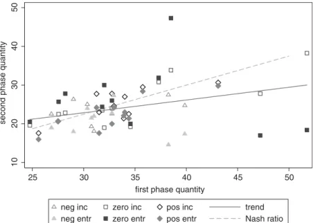
Yet, as Figure 16.3 illustrates, aggregates per treatment conceal a more complex story. In this figure, each marker is the mean quantity set by the two incumbents or the entrant in one group. There is quite some variation that is hidden by looking at averages only. In phase 1 of the Cournot market, quantity choices have mean 33.57, but standard deviation 10.34. Quantity choices in the second phase of the experiment heavily depend on experiences from the first phase. Independent of treatment, what the group has experienced while the market was a duopoly is a strong predictor of quantity choices after the entrance of the new competitor. Suppliers only adjust quantities to reflect greater competition: the trend line is close to 75% of the average quantity in the first 10 periods (which would be the quantity ratio of a triopoly com- pared to a duopoly, as predicted by standard theory). As the distribution of hollow (incumbents) versus solid markers (entrants) shows, market history matters for old

010203040

quantity

1 2

neg zero pos neg zero pos

quantity choices over phase, treatment and role

incumbent entrant

Figure 16.2:Aggregate quantity choices.

Table 16.1:Descriptive statistics.

Phase Phase

neg zero pos neg zero pos

incumbent .

(.)

.

(.)

.

(.)

.

(.)

.

(.)

.

(.)

entrant .

(.)

.

(.)

.

(.) Note: standard deviations in parenthesis

and new market participants. We note that this history effect is in line with the only other experiment we are aware of that tests market entry (Goppelsroeder 2009).

Overall, we can conclude that while there is a lot of idiosyncrasy regarding market competitiveness, Nash equilibrium goes a long way to predict average quantities and average differences of competitive pressure in our duopoly and triopoly settings.

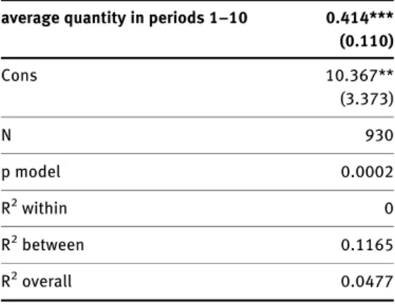
The visual impression that local market competitiveness in periods 1 – 10 mat- ters is supported by statistical analysis (see Table 16.2).

1020304050

second phase quantity

25 30 35 40 45 50

first phase quantity

neg inc zero inc pos inc trend

neg entr zero entr pos entr Nash ratio

Figure 16.3:Dependence on local conditions.

Notes: x-axis: mean quantity sold by the two members of the duopoly, in periods 1–10 y-axis: mean quantity sold in periods 11–20

separately for incumbents (hollow markers) and for entrants (solid markers) trend: linear prediction

Nash ratio: 3/4 of first phase quantity

18 We revert to regression analysis since we want to show that choices in periods 11–20 are ex- plained by the average quantity this group had chosen before the third supplier enters the market.

We have data from choices, nested in individuals, nested in groups. Dependence within individuals is captured by the random effect. The additional source of dependence at the group level is captured by clustering standard errors at this level. The fact that the Hausman test does not turn out significant shows that we are justified in preferring the more efficient random effects model over a model with individual fixed effects. The coefficient of the average quantity in phase 1 is smaller than 0.75 since the model has a constant. If we estimate the same model (as a population averaged regression) with- out a constant, the coefficient comes very close to the theoretical expectation and is 0.714.

This gives us:

Result 1: If a new competitor enters a repeated Cournot duopoly market, higher pre-entry quantity is associated with higher post-entry quantity.

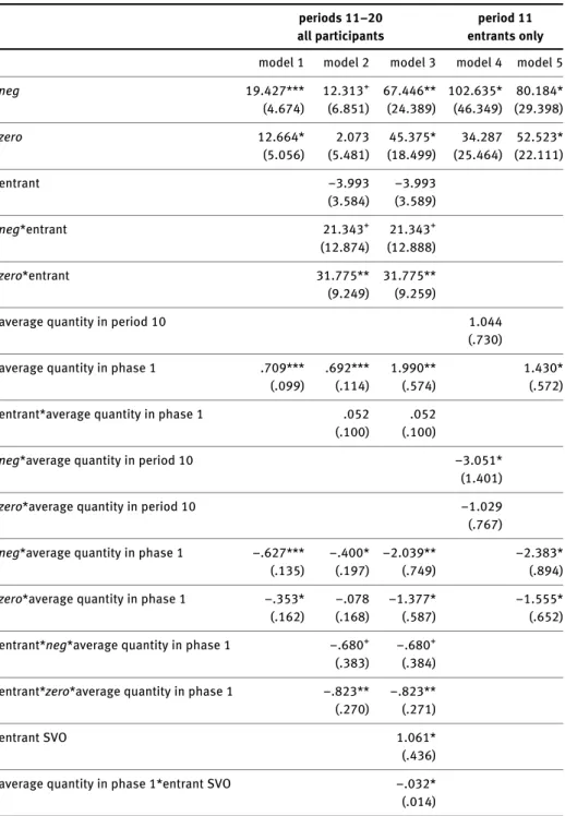
Knowing that local market conditions matter, we revisit the effects of our manipu- lation in Table 16.3.

The constant of the regression in Model 1 predicts the amount a firm would sell in the Positive treatment if the average amount sold in this group in the first 10 periods had been 0. Of course, as Figure 16.3 shows, in the experiment there has been no such market. The regression generalizes to the population of Cournot du- opolies observed by entrants. If we plug in the average amount sold in the first 10 peri- ods from all 11 markets where the entrant has a positive social value orientation score (32.973, Table 16.1), the regression predicts that, in the Positive treatment, firms on av- erage sell 24.02 units,

which comes pretty close to the Nash quantity of 25 units.

From the significant positive main effects of treatments Negative and Zero we learn that, overall, the market is more competitive if the entrant is rivalistic or self- ish, compared with a market where the entrant has a preference to avoid payoff dif- ferences. Yet this treatment effect is indeed conditional on the competitiveness before market entry. The significant negative interactions show that the translation effect is most pronounced if the entrant has a positive social value orientation

Table 16.2:Effect of local conditions.

average quantity in periods– .***

(.)

Cons .**

(.)

N 

p model .

R^within 

R^between .

R^overall .

Notes: dependent variable: quantity, data from periods 11–20 random effects, robust standard errors clustered at the group level Hausman test insignificant on mirror model with period as additional regressor (to enable fixed effects estimation) standard errors in parenthesis * = p < .05

19The fact that“overall”all models seem to explain little variance is an artefact of the fact that, by their design, these models only explain between, not within variance.

20.638 + 32.973 * .709 = 24.02.

Table 16.3:Treatment effects conditional on local conditions.

periods–

all participants

period

entrants only

model model model model model

neg .***

(.)

.⁺ (.)

.**

(.)

.* (.)

.* (.)

zero .*

(.)

.

(.)

.* (.)

.

(.)

.* (.)

entrant −.

(.)

−.

(.)

neg*entrant .⁺

(.)

.⁺ (.)

zero*entrant .**

(.)

.**

(.)

average quantity in period .

(.) average quantity in phase .***

(.)

.***

(.)

.**

(.)

.* (.)

entrant*average quantity in phase .

(.)

.

(.)

neg*average quantity in period −.*

(.)

zero*average quantity in period −.

(.) neg*average quantity in phase −.***

(.)

−.* (.)

−.**

(.)

−.* (.) zero*average quantity in phase −.*

(.)

−.

(.)

−.* (.)

−.* (.) entrant*neg*average quantity in phase −.⁺

(.)

−.⁺ (.) entrant*zero*average quantity in phase −.**

(.)

−.**

(.)

entrant SVO .*

(.) average quantity in phase*entrant SVO −.* (.)

score. The more the market was competitive pre-entry, the less it becomes even more competitive through the entry of a new competitor with rivalistic or selfish preferences. In fact, the pro-competitive effect of the entrant holding rivalistic pref- erences only plays itself out if the average quantity pre-entry was at or below 31 units

; recall that the Nash quantity for the duopoly is 33 units. Likewise, if the en- trant is selfish, entry only has a pro-competitive effect if the average quantity pre- entry was at or below 36 units.

Yet in both treatments, the pro-competitive effect of entry is pronounced if the duopoly was perfectly collusive. The model predicts that quantity is 3.752 units higher if a rivalistic firm enters a collusive market, and 3.839 units higher if a selfish firm enters.

Model 2 splits the analysis by entrants and incumbents. The picture nicely clears if, in model 3, we additionally control for the precise social value orientation score of the entrant, and how it interacts with the competitiveness of the market before she enters. The following discussion focuses on this model. The implications are easiest to see in the marginal effect of the Negative and Zero treatments that are reported in Figure 16.4. If we find a significantly positive effect of treatment, the

Table 16.3(continued )

periods–

all participants

period

entrants only

Cons .

(.)

.

(.)

−.* (.)

−.

(.)

−.

(.)

N     

p model <. <. <. . .

R^within   

R^between . . .

R^overall . . . . .

Notes: regression equations for all models in Appendix II dependent variable: quantity models 1–3:

data from periods 11–20, models 4–5: data from period 11 models 1–3: data from incumbents and entrants, models 4–5: data from entrants only models 1–3: random effects, robust standard errors clustered at the group level Hausman test insignificant on mirror models with period as additional regressor (to enable fixed effects estimation) SVO: social value orientation, i.e. score from ring measure test treatment: reference category:positivestandard errors in parenthesis *** p < .001, **

p < .01, * = p < .05,⁺p < .1

21 19.427/.627 = 30.984.

22 12.664/.353 = 35.875.

2319.427–25*.627 = 3.752; 12.664–25*.353 = 3.839.

−60

−40

−20 0 20 40

marginal effect of treatment

2530354045 av quantity phase 1 incumbententrant

neg

−40

−20 0 20

40

marginal effect of treatment

2530354045 av quantity phase 1 incumbententrant

zero Figure16.4:Marginaleffectoftreatment,conditionalonroleandcompetitiveness. Note:marginaleffectsfrommodel3ofTable16.3

rivalistic or selfish personality of the entrant has a pro-competitive effect. This holds true for both treatments and roles, but only if, pre-entry, the market was col- lusive.

With this qualification, we reject our null hypothesis H

and infer that the alternative hypothesis H

captures the data. We also note that the asymmetric re- sponse of selfish (Zero) and rivalistic (Negative) entrants to their observations from the first 10 periods is well in line with their playing best responses, assuming that incumbents will only adjust to the fact that one more supplier enters the market (but not reach equilibrium choices themselves). In the Appendix I we show this formally.

To see whether the social preferences of entrants are indeed critical, we consider period 11 in isolation, i.e. the first period after entry. Overall, and if we confine the analysis to incumbents, we do not find any treatment effects, even if we interact treatment with the average quantity chosen in the respective group in period 10 (i.e.

directly before entry), or during all of periods 1 – 10. But we do see a strong effect of the Negative treatment if we separately analyze choices of entrants (Model 4 of Table 16.3). We also see an effect of the Zero treatment if we replace average choices in period 10 with average choices in periods 1 – 10 (Model 5 of Table 16.3). Recall that incumbents had no information about the criterion for selecting entrants. Models 4 and 5 not only show that our manipulation worked. Together with Models 1 – 3 we also see how a maverick changes the market: immediately after entry, she behaves according to her preferences; in later periods, incumbents react to this experience.

Thus far our data suggest that a rivalistic and a selfish entrant have pretty much the same effect on competitiveness. To see whether this is indeed true, we use the following approach: individually for each incumbent we regress quantities sold in the first phase on time. This procedure gives us for each individual incum- bent the trend, had there not been entry. From these regressions, for each individ- ual we derive an out of sample prediction for the remaining 10 periods. We adjust the predicted quantity to the market entry of one more supplier by multiplying it by the theoretically predicted ratio of ¾ (see above). Note that the prediction is flat if, pre entry, the market had already reached equilibrium. However, inspecting the raw data, it seems that most duopoly markets had not yet stabilized. Only 17 of 62 incumbents did not change the quantity over periods 6 – 10.

Figure 16.5 shows the difference, per treatment and period, between the mean actual and predicted quantity. In the Positive treatment, actual quantities are much higher than the prediction. In the Zero treatment, actual quantities exhibit more variance, but have about the same level as the prediction. By contrast in the Negative treatment, and only in this treatment, for all periods but the final actual

24 The marginal effects of Figure 16.4 also explain the seemingly contradictory descriptive finding that, in theNegativetreatment, entrants on average choose smaller quantities than incumbents, Table 16.1: entrants only bid more than incumbents if the market had been collusive.

25We are grateful to an anonymous referee for suggesting this approach.

−4

−2 0 2 4 6

mean difference between phase 2 and phase 1

101214161820 Period

neg

−4

−2 0 2 4 6

mean difference between phase 2 and phase 1

101214161820 Period

zero

−4

−2 0 2 4 6

mean difference between phase 2 and phase 1

101214161820 Period

pos Figure16.5:Effectofentryonchoicesofincumbents. Notes:periods11–20onlydependentvariable:difference,pertreatmentandperiod,betweenthemeanpredictedandactualquantity

quantities are below the predicted trend.

We conclude that, depending on the so- cial preferences of the entrant, incumbents come under additional competitive pres- sure and react by reducing the quantity they sell, as predicted by our model.

Overall, this gives us:

Result 2: Conditional on pre-entry local market competitiveness, a Cournot market is more competitive if the entrant is rivalistic.

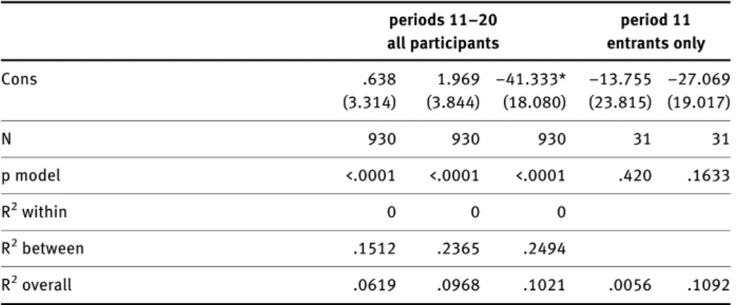
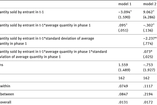
In the final step, we want to understand in which ways rivalistic entrants disci- pline incumbents. To that end we take a closer look at dynamics in the Negative treatment. The dependent variable is changes in incumbents ’ choices from one pe- riod to the next.

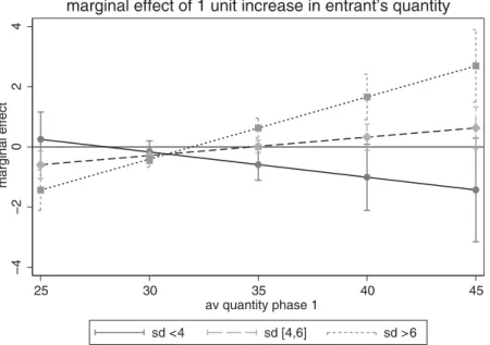
Model 1 of Table 16.4 shows that incumbents, on average, reduce their own con- tributions in reaction to high contributions of the entrant (p = .088), as predicted by our theory. The weakly significant interaction effect (p = .099) indicates that the ef- fect is the more pronounced the more the market was collusive before the third sup- plier entered. Model 2 and the marginal effects reported in Figure 16.6 show that the effect requires some degree of discord among the incumbents though.

If the standard deviation of quantity choices in this group and every period of phase 1 was low on average (range [2.828, 7.778]), incumbents do not significantly reduce their quantity in reaction to a high quantity sold by the entrant. This suggests that a duopoly that has successfully established a common norm of behavior is more resil- ient to attempts of a maverick to break up collusion; indeed, previous research has shown that homogeneous cooperation across agents is less vulnerable to being de- stabilized (e.g. Brosig, Weimann, and Ockenfels 2003).

16.5 Conclusion

Antitrust authorities are not only concerned with market power. They are also atten- tive to firm-specific heterogeneity in market behavior. They are particularly pleased if

26The visual impression is supported by statistical analysis. If we regress the difference between the actual quantity and the out of sample prediction on treatment, and choose theNegativetreat- ment as reference category, the constant informs us about the treatment effect for this treatment. If we use all 10 periods of the second phase, the constant is–1.641, but not significantly different from zero (p = .151). If we repeat the analysis for periods 11–19, however, the constant is–2.392, p = .002, which supports our claim. In neither regression, the net effect of constant + treatmentZerois significantly different from zero (p = .9016 in the first and p = .8519 in the second regression). We do, however, acknowledge that the treatment effect diminishes over time. If we repeat the regres- sion, now interact treatment with period, and subsequently test the net effect of the constant + pe- riod, the result is significantly different from zero for periods 11–16 only. The additional regressions are available from the authors upon request.

27Further controlling for the mean quantity sold individually by each incumbent, or replacing the standard deviation with this measure, does not yield significant effects.

they identify especially aggressive firms. In this paper we experimentally investigate a cause for such “ maverick ” behavior that transcends pecuniary incentives: an indi- vidual may derive utility from relative, not only from absolute payoff.

In our experiment, we do indeed find that market entry by a participant with a particularly rivalistic attitude makes the market more competitive, improving con- sumer welfare and hampering incumbents ’ profits. Yet this result only holds condi- tional on the level of competition pre-entry. The entry of a “ maverick ” is socially most beneficial when it is most needed, i.e. when the market was collusive. This suggests that mavericks can play an important role for entertaining competitive markets, and so competition authorities may be indeed well-advised to appreciate this role in their policies.

We of course do not claim a one to one mapping of the behavior of students in the lab (which we test) to the behavior of firms in markets. Firms are highly aggregate

Table 16.4:Reaction of incumbents to quantity choices of entrants innegtreatment.

model model

quantity sold by entrant in t- −.⁺

(.)

.⁺ (.) quantity sold by entrant in t-*average quantity in phase .⁺

(.)

−.⁺ (.) quantity sold by entrant in t-*standard deviation of average

quantity in phase

−.* (.) quantity sold by entrant in t-*average quantity in phase*standard

deviation of average quantity in phase

.* (.)

cons .

(.)

−.

(.)

N  

R^within . .

R^between . .

R^overall . .

Notes: dv: quantity(t)–quantity(t-1) of incumbents data fromnegtreatment individual fixed effects, since Hausman test turns out significant robust standard errors, clustered for groups, in parenthesis *** p < .001, ** p < .01, * = p < .05,⁺p < .1

28 The fact that we do not have even stronger findings might also result from the composition of our sample. In line with previous experimental results (Liebrand and McClintock 1988), only a mi- nority of our participants is willing to give up some income for increasing the distance in payoff to their favor. With one exception, even those who do are only mildly rivalistic.

corporate actors (for a survey of the experimental research specifically addressing such actors see Engel 2010), and decision making is rarely individual but rather based on some aggregation of team preferences; suppliers in a real market of three do not interact anonymously and underlying preferences of both, incumbents and mavericks may be subject to selection effects; and markets are differently organized and structured – to name only some obvious simplifications. But in line with a rich literature on experimental oligopoly markets (see the meta-study by Engel 2015) we believe that such evidence provides a useful starting point for analyzing the behavior of firms. Eventually, individuals decide for firms. It is therefore not unlikely that be- havioral traits of these individuals carry over to the behavior of the firms for whom they act. Managers are not only selected for their competence and connections, but also for their personalities. It is not unlikely that a firm selects particularly aggressive individuals if it intends to act aggressively in the market. Moreover, firms as corpo- rate entities may themselves, in different degrees, care about relative, not only about absolute payoff. One reason is the embeddedness of some firms into financial mar- kets, possibly also into a market for corporate control. In these markets, comparative performance may be a very relevant signal, whereas in other markets that might be less so.

That said, an experiment will not be able to settle the policy debate over mav- ericks. Experiments are only tools for identifying potential effects. But we add an

−4−2024marginal effect

25 30 35 40 45

av quantity phase 1

sd < 4 sd [4,6] sd > 6

marginal effect of 1 unit increase in entrant’s quantity

Figure 16.6:Reaction of incumbents to quantity choices of entrants innegtreatment.

Notes: marginal effects of 1 unit lagged increase in entrant’s quantity on change in incumbents’ quantity from model 2 of Table 16.4

important argument to this policy debate. Maverick choices may be expected, they may be sustainable, and they may affect market outcomes, even in the absence of a pecuniary incentive to act aggressively. Anti-trust authorities have no reason to stop searching for, or protecting, maverick behavior, even if it does not seem to be grounded in sound profit incentives of the firm in question.

A second finding is of even greater importance for anti-trust policy: maverick behavior is not to be expected irrespective of context. When they face tough compe- tition, even individuals (firms) otherwise inclined to compete aggressively are likely to hold back. We have of course only shown this for maverick behavior resulting from rivalistic preferences. But one should a fortiori expect a disciplining effect of a competitive environment on mavericks that have an incentive to outperform others (for instance since their income is tied to market share): by definition, maverick be- havior reduces absolute profit. For anti-trust, this insight matters in merger control.

Not so rarely, mergers between conglomerate firms reduce competition in one, but increase competition in another market. In principle, it makes sense to balance out these effects. But if the merger enables entry into a new market and competition in this market is intense, the merger is unlikely to increase consumer welfare, even if the entrant has an incentive to bid aggressively.

Appendix I: Model

In the general case of a Cournot market with linear demand, intercept m, and n sup- pliers, all with marginal cost of zero, the Cournot-Nash quantity is given by:

q

= m n + 1

We now assume that the utility of the rivalistic supplier e (given that the other two suppliers make identical profits π

, which will be the case in equilibrium) is given by u

= π

+ ð n − 1 Þ γ ð π

− π

Þ

= ð 1 + 2 γ Þ ð m − ð n − 1 Þq

− q

Þq

− 2 γ ð m − ð n − 1 Þq

− q

Þq

Profit for one of the incumbents is now given by π

= m − q

− ð n − 2 Þq

− q

q

Taking first order conditions, and solving the resulting system of equations, we get q

= q

= m ð 2 γ + 1 Þ

2 γ n + n + 1 + 4 γ , q

= m ð 4 γ + 1 Þ 2 γ n + n + 1 + 4 γ

E.g., with the parameters of the experiment, and letting the entrant be mildly rival-

istic, i.e. with γ =

, we get q

= q

= 22 . 22 , q

= 33 . 33. The rivalistic player is better off

the larger γ , that is the more she is rivalistic. If all sellers hold standard preferences, in equilibrium they sell Q

= nq

=

units. If one seller is rivalistic, total quantity is given by

Q

= ð n − 1 Þ m ð 2 γ + 1 Þ

2 γ n + n + 1 + 4 γ + m ð 4 γ + 1 Þ 2 γ n + n + 1 + 4 γ

which is larger than Q

for any γ > 0; with γ = 0 , Q

= Q

. Hence consumer welfare increases if there is a rivalistic player.

Qualitatively similar results are obtained if we also allow incumbents to be ri- valistic as shown below, if we keep the assumption that the entrant is more rivalis- tic γ

≥ γ

.

Specifically, let us assume that α = γ

< γ

= γ . Taking first order conditions, and solving the resulting system of equations, we get

q

= q

= m ð 4 αγ + 2 α + 2 γ + 1 Þ 4 αγ n + 2 α n + 2 γ n + n + 1 + 4 γ ,

q

= m ð 4 αγ + α + 4 γ + 1 Þ 4 αγ n + 2 α n + 2 γ n + n + 1 + 4 γ

Similar to our previous results, each incumbent sells less than the entrant, and con- sumer welfare increases both in α and γ .

Our hypotheses are based on the assumption that preferences are common knowledge, and that all suppliers maximize utility. This is not what we find in the experiment. Visibly many duopolies are out of equilibrium, and entrants react to this. We therefore also report best responses of entrants, assuming that incumbents will only adjust quantities to the entry of one more supplier (i.e. will choose q

= . 75 * q

, where numbers 2 and 3 stand for the number of suppliers). If the entrant maximizes profit (is selfish), she will then choose the following best response

q

= 1

2 ð m − ð n − 1 Þ . 75 * q

Þ

or, with the parameters of the experiment, 50 − . 75 * q

. Note that, if the duopoly was in equilibrium, 75 * q

= 25, so that the best response is the equilibrium. Hence the

29In fact, the result can be generalized by noting that our model is related to the model by Fehr and Schmidt (1999). The difference is that the Fehr-Schmidt model allows players to also suffer from advantageous inequality. However, as long as the entrant is assumed to be more aggressive than the incumbents, the incumbents will in equilibrium always fall behind the entrant and so never experience advantageous inequality. Since the utility from the difference between one’s own payoff and the payoff of a peer is not constrained to positive differences, our utility also captures disutility from falling behind one’s peers. So, technically, this leads to a market ofnplayers who all hold preferences as we assume above.

model predicts that entrants choose a larger quantity only if the duopoly was collu- sive. This fits the data from the Zero treatment very well, Figure 16.4.

If entrants are rivalistic, the best response to the expectation that incumbents will only adjust to the fact that one more supplier is in the market is given by maxi- mizing the utility, assuming q

= . 75 * q

. In generic notation the best response is given by

q

= m + ð n − 1 Þ . 75 * q

+ ð n − 1 Þ γ ð m − ð n − 2 Þ . 75 * q

Þ 2 + ð 2n − 2 Þ γ

With the parameters of the experiment, this simplifies to q

= 50 − . 75 * q

+ ð 100 − . 75 * q

Þ γ

1 + 2 γ

Note that this quantity is below the Nash quantity for large q

and/or for small γ .

This fits the results from Figure 16.4 very well.

Tablemodelquantityittj>10=β0+β1*treat+β2*meanquantitygjt<11 +β3*treat*meanquantitygjt<11 +εi+εit Tablemodelquantityittj>10=β0+β1*treat+β2*meanquantitygjt<11 +β3*treat*meanquantitygjt<11 +β4*entrant+β5*treat*entrant+β6*entrant*meanquantitygjt<11 +β7*entrant*treat*meanquantitygjt<11 +εi+εit Tablemodelquantityittj>10=β0+β1*treat+β2*meanquantitygjt<11 +β3*treat*meanquantitygjt<11 +β4*entrant+β5*treat*entrant+β6*entrant*meanquantitygjt<11 +β7*entrant*treat*meanquantitygjt<11 +β8*entrant′sSVO+β9*entrant′sSVO*meanquantitygjt<11 +εi+εit Tablemodelðquantityit−quantityi,t−1Þtj>10,incumbent=β0+β1*quantityt−1,entrant+ β2*quantityt−1,entrant*meanquantitygjt<11 +εi+εit Tablemodelðquantityit−quantityi,t−1Þtj>10,incumbent=β0+β1*quantityt−1,entrant+ β2*quantityt−1,entrant*meanquantitygjt<11 +β3*quantityt−1,entrant*meansdmeanquantitygjt<11 +β4*quantityt−1,entrant*meanquantitygjt<11 *meansdmeanquantitygjt<11 +εi+εit

Appendix II: Regression equations

Appendix III: Instructions

a) Instructions: First session (1) General instructions

Thank you for taking part in our experiment. From your invitation you already know that the experiment is in two parts. These instructions explain the first part of the experiment, taking place today. We will pay you your earnings from today ’ s part of the experiment at the end of today ’ s session. However, it is very important for our experiment that you also participate in the second session.

You can earn money in this experiment. How much you earn depends on your decisions and the decisions of other participants. Your earnings will be paid to you in cash at the end of the experiment.

Please switch off your mobile phone now, and please do not communicate any longer with the other participants as of this moment. Should you have a question about the experiment, please raise your hand. We will come to you and answer your query.

Today ’ s part of the experiment consists of different sections. In these instruc- tions, we explain the first section. For the following sections, you will find your in- structions on the screen in front of you.

In order for us to keep track of your performance in the second part of the ex- periment, we would ask you please to generate an identification code at the end of the experiment, and to enter this code on your computer screen. We will use this identification code to connect your data from the first and second parts of the ex- periment. At no time do we know your name or address. Only the laboratory admin- istration has that information. However, the laboratory administration does not know your decisions. This way we can ensure that anonymity is guaranteed at all times. Please write down this number and bring it with you when you are invited to the second experiment. At the beginning of the the second experiment, we will ask you to enter this number on your computer screen. If you enter the wrong number, you cannot take part in the second experiment. Therefore, please check whether you have made a note of the correct number.

(2) First section

We are now going to ask you to make several decisions. For this to happen, you will

be randomly matched with another participant. You can allocate Taler to this par-

ticipant and to yourself in the course of several distribution decisions. In order to

do this, you will have to choose repeatedly between two distributions, X and Y

(e.g., distribution X: 10 Taler for yourself and 12 Taler for the other player; and dis-

tribution Y: 8 Taler for yourself and 20 Taler for the other player). The Taler you

allocate to yourself are paid out to you at the end of the experiment, at a rate of 100

Taler = 1 € . At the same time, you are also randomly matched with yet another exper-

iment participant who, in turn, can allocate Taler by way of distribution decisions.

This participant is not the same as the one to whom you can allocate Taler. The Taler allocated to you are also transferred to your account and paid out to you at the end of the experiment, at a rate of 100 Taler = 1 € .

The individual decision tasks will look like this: