Veröffentlichungen der DGK
Ausschuss Geodäsie der Bayerischen Akademie der Wissenschaften
Reihe C Dissertationen Heft Nr. 822
Sujata Goswami
Understanding the sensor noise in the GRACE range-rate observations by analyzing their residuals
München 2018
Verlag der Bayerischen Akademie der Wissenschaften
ISSN 0065-5325 ISBN 978-3-7696-5234-5
Veröffentlichungen der DGK
Ausschuss Geodäsie der Bayerischen Akademie der Wissenschaften
Reihe C Dissertationen Heft Nr. 822
Understanding the sensor noise in the GRACE range-rate observations by analyzing their residuals
Von der Fakultät für Bauingenieurwesen und Geodäsie der Gottfried Wilhelm Leibniz Universität Hannover
zur Erlangung des Grades Doktor-Ingenieur (Dr.-Ing.)
genehmigte Dissertation
Vorgelegt von
M.Tech. Sujata Goswami
Geboren am 16.07.1990 in Modinagar, India
München 2018
Verlag der Bayerischen Akademie der Wissenschaften
ISSN 0065-5325 ISBN 978-3-7696-5234-5
Adresse der DGK:
Ausschuss Geodäsie der Bayerischen Akademie der Wissenschaften (DGK) Alfons-Goppel-Straße 11 ● D – 80539 München
Telefon +49 – 331 – 288 1685 ● Telefax +49 – 331 – 288 1759 E-Mail post@dgk.badw.de ● http://www.dgk.badw.de
Prüfungskommission:
Vorsitzender: Prof. Dr.-Ing. Udo Nackenhorst Referent: Prof. Dr.-Ing. Jürgen Müller Korreferenten: Prof. Dr.-Ing. Torsten Mayer-Gürr
Prof. Dr.-Ing. Christian Heipke Tag der mündlichen Prüfung: 12.07.2018
© 2018 Bayerische Akademie der Wissenschaften, München
Alle Rechte vorbehalten. Ohne Genehmigung der Herausgeber ist es auch nicht gestattet,
die Veröffentlichung oder Teile daraus auf photomechanischem Wege (Photokopie, Mikrokopie) zu vervielfältigen
ISSN 0065-5325 ISBN 978-3-7696-5234-5
Abstract
The gravity recovery and climate experiment (grace) mission has successfully used the inter-satellite ranging technology to determine the time-variable gravity field of the earth. After staying in orbit for more than 15 years, the mission has been decommissioned in october 2017. However, the requirements to meet the grace baseline accuracy have not yet been achieved due to the presence of various error sources. One of the major sources partially is mis-modeled errors of the sensor observations. Such errors can be seen in the post-fit range-rate residuals. Our goal is to understand the errors in the range-rate observations and analyze the corre- sponding residuals to identify mis-modeled sensor errors. Specifically, an analysis of the attitude, ranging and accelerometry errors in the grace satellite observa- tions and in the corresponding range-rate residuals is presented. By analyzing the range-rate residuals the knowledge of systematic effects of the sensors affecting the measurements are gained.
In this work, it is shown that the range-rate residuals are highly dominated by
high frequency (>20 mhz) system noise. In particular, phase errors of the k-band
frequencies of both spacecraft lead to the noise in the high frequencies of the range-
rate residuals. The error contribution due to such effects may reach up to 30 % of
the total error. Further, while analyzing the range-rate residuals, it has been found
that the highest attitude error contributors in the range-rate observations are the
range-rate antenna phase center offset corrections. The contribution of those atti-
tude errors can be as high as 25 % of the total error. The analysis of low frequency
residuals (≈ 1 cpr to 30 cpr) shows the dominance of instrument temperature fluc-
tuations, satellite maneuvers dependent errors and errors due to spacecraft shadow
transitions propagated via the accelerometers. Range-rate residuals in these fre-
quencies also contain a considerable amount of errors of the geophysical background
models and of the attitude. As the range-rate residuals are dominated by system-
atic errors from the sensors, there is still a scope of improvement in the modeling of
observation noise and in the instrument re-calibration approaches in order to mini-
mize the error contribution. A similar strategy will be helpful for the analysis of the
laser ranging instrument and k-band ranging residuals of the recently launched
grace-follow on mission.
Zusammenfassung
Die satellitenmission “Gravity Recovery and Climate Experiment” (GRACE) wurde erfolgreich zur bestimmung des zeitlich variablen erdschwerefeldes mittels satelliten-abstandsmessung verwendet. Die mission wurde im October 2017 been- det, nachdem die satelliten mehr als 15 Jahre im orbit waren. Dennoch konnte die vorgesehene genauigkeit aufgrund verschiedener fehlerquellen bisher nicht erreicht werden. Eine der wichtigsten fehlerquellen sind fehlerhafte modelle der messdaten verschiedener sensoren. Diese fehler sind sichtbar in den post-fit residuen der abstandsänderungsraten (“range-rates”). Unser ziel ist es, die fehler in diesen range-rate messungen zu verstehen und die entsprechenden residuen zu analysieren, um fehler in den sensor-modellen zu identifizieren. Insbesondere präsentieren wir eine analyse der fehler im zusammenhang mit der ausrichtung der satelliten, der abstands- sowie der akzelerometermessungen, sowohl in den messdaten als auch in den entsprechenden residuen. Durch die analyse der range-rate residuen kann information über systematische effekte der sensoren, welche die messungen beein- flussen, gewonnen werden.
In dieser arbeit wird gezeigt, dass die range-rate residuen dominiert werden von hochfrequentem ( > 20 mhz) systemrauschen. Insbesondere wird das rauschen in hohen frequenzen durch phasenrauschen des k-band instruments (auf beiden satelliten) verursacht. Diese art von fehler macht bis zu 30% des gesamtfehlers aus. Ferner wurde festgestellt, dass der größte teil des fehlers in den range-rate residuen, der von der ausrichtung der satelliten abhängt, durch die korrekturterme des phasenzentrums (“antenna offset corrections”) verursacht wird. Dieser fehler kann bis zu 25% des gesamtfehlers aus.Die analyse der residuen im niedrigfrequenz- bereich (etwa 1 bis 30 cpr ) zeigt drei dominierende fehler, verursacht durch temperaturschwankungen, satellitenmanöver und licht-schatten-durchgänge via ak- zelerometermessungen. Die residuen enthalten außerdem fehler in den geophysikalis- chen hintergrundmodellen sowie von der ausrichtung der Satelliten abhängige fehler.
Da die residuen von systematischen fehlern der sensoren dominiert werden, gibt
es verbesserungsmöglichkeiten durch bessere modellierung des instrumentrauschens
und durch erweiterte ansätze zur rekalibrierung der instrumente. Eine ähnliche
strategie wird auch hilfreich sein für die analyse der laser ranging und k-band
ranging residuen der grace-follow on mission, die im Mai 2018 gestartet wurde.
Acknowledgements
I would like to thank Prof. Jakob Flury for giving me the opportunity to work on this topic. I am highly thankful to Prof. Torsten Mayer-Gürr not only for being my second supervisor but also for providing me the access to necessary computational resources due to which my work pace improved tremendously. I am also thankful to Dr. Matthias Weigelt for agreeing to be my ancillary supervisor and helping me from time to time in my research. He was also a very nice friend during my Ph.D.
whose moral support was of great help.
Dear Balaji and Jayani, I could not have made it without both of you. You two were a big moral support during my good as well as bad times in Hannover. Balaji, I thank you so much for being an excellent collaborator. I found your doors always open for discussions. Those discussions helped me a lot in improving me as a scien- tist and my work, both.
Dear Tamara, this work would not have had come to this end without you. Dis- cussions with you helped me alot in kicking off my work. Your help in patiently explaining the complex data characteristics in an easy way were of big help. Not only just scientific help, you were also a great moral supporter during my tough times in Ph.D. A big thanks to all of you.
I am highly thankful to Prof. Karsten Danzmann, Fumiko Kawazoe, Prof. Jürgen Müller and all the IfE members for being so generous to me in the time of need. I could not see myself writing this draft without the support I got from all of them.
Although, Hannover had been my main work place, I was also visiting the group of Prof. Torsten Mayer-Gürr in TU Graz time to time. I owe a big thanks to the Graz team - Matthias Ellmer, Beate Klinger, Saniya Behzadpour, Andreas Kvas and Norbert Zehentner for being such nice hosts at TU Graz and always patient in replying to my emails.
In the last but always first, I am grateful to God who gave me such lovely and supportive parents and siblings. It was just so lucky to have my partner Saurabh by my side all the time during the Ph.D. He was always my pillar of strength during the tough research times.
Hannover, August 2018
Sujata Goswami
Contents
Abstract 1
Zusammenfassung 3
Acknowledgements 5
I Introduction 11
1 Introduction 13
1.1 State of the art . . . 14
1.2 Objectives . . . 21
2 Gravity Recovery And Climate Experiment Mission 23 2.1 Introduction . . . 23
2.2 Applications . . . 23
2.3 The GRACE observation system . . . 24
2.4 Global gravity field parameter estimation from GRACE observations 28 2.4.1 Gravity field representation . . . 28
2.4.2 Gravity field modeling . . . 28
2.5 Analysis kit used for studying the residuals . . . 35
2.5.1 Degree amplitudes . . . 35
2.5.2 Power Spectral Density (PSD) . . . 35
2.5.3 Time-series analysis . . . 36
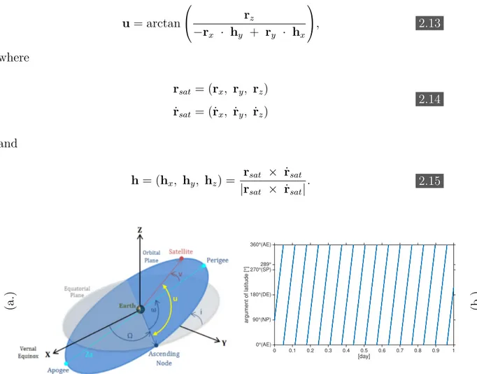
2.5.4 Argument of latitude . . . 37
2.5.5 Satellite ground tracks . . . 39
II Analysis of K-band range-rate residuals 41 3 Inter-satellite pointing errors in range-rate residuals 43 3.1 What is inter-satellite pointing? . . . 43
3.2 GRACE attitude - its characteristics and errors . . . 46
3.3 Attitude error propagation into the range-rate observations . . . 54
3.3.1 Error propagation via antenna offset corrections . . . 54
3.3.2 Error propagation via linear accelerations . . . 58
3.4 Post-fit residual analysis with focus on attitude errors . . . 60
3.5 How do attitude errors affect gravity field solutions? . . . 65
3.5.1 Simulation scenario . . . 65
3.6 Summary . . . 71
4 Inter-satellite ranging errors in range-rate residuals 73 4.1 Inter-satellite ranging . . . 73
4.2 Inter-satellite ranging errors . . . 75
4.3 Post-fit residual analysis with focus on ranging errors . . . 78
4.4 Impact of high-frequency errors on the gravity field solutions . . . 89
4.5 Summary . . . 92
5 Accelerometer errors in range-rate residuals 93 5.1 GRACE accelerometer . . . 93
5.2 Errors and characteristics of GRACE accelerometer observations . . . 94
5.3 Range-rate residual analysis with focus on accelerometer errors . . . . 104
5.4 Summary . . . 117
III Conclusions 121 6 Conclusions 123 Appendices 127 A Inter-satellite pointing angles and the satellite panels 129 A.1 Computation of GRACE inter-satellite pointing angles . . . 129
A.2 Satellite panels . . . 132
Bibliography 144
Curriculum Vitae 145
Introduction
Introduction
The study of features of the gravity field of the earth has always been one of the primary interests of geodesy. The earth’s gravity field and changes in it reflect mass changes inside and on the surface of the earth.
As an example, earth’s gravity measurements are used to get information about the shape of the geoid. Variations of the gravity field reflect continental water storage changes, ice mass balance changes, glacial isostatic adjustment and sea level changes.
All these phenomena influence the human life on the earth, directly or indirectly, and their accurate knowledge depends on the accuracy of the gravity measurements.
Therefore, precise knowledge of the gravity field is not only necessary for geodetic science but also an important requirement for climate science.
In the beginning of the 20
thcentury, gravity measurements were carried out on ground using instruments called gravimeters. These instruments were capable of measuring gravity changes as point observations. A major limitation of the gravime- ters was and still is, that they could not be used over a large region or on a global scale. This goal was first accomplished later in the 20
thcentury with the use of satellites. Use of artificial satellites for geodetic purposes was introduced during 1950s after the launch of sputnik in 1957 and explorer in 1958. These missions allowed the successful determination of the flattening of the earth, e.g. Heiskanen and Moritz (1967).
The first dedicated geodetic satellite was anna-1b launched on 31 October 1962 by national aeronautics and space administration (nasa) and the department of defense which led to an accurate determination of the very low-degree spherical harmonic coefficients of the geopotential, the general shape of the geoid. The first decade of the 21
stcentury was dedicated to measure the earth’s gravity field with satellite missions, e.g., satellite laser ranging (slr) missions, champ, grace and goce.
GFZ-1 (geoforschungszentrum potsdam) is an example of satellites launched to
determine the gravity field of the earth along with the determination of its rotation
and the precise position of the spacecraft. These satellites were equipped with retro-
reflectors to be illuminated from the ground by the global network of the slr system
(GeoForschungsZentrum, 2018).
CHAMP (challenging and minisatellite payload) was the first dedicated and suc- cessful mission launched aiming at the measurement of the gravity field. It was based on orbit tracking and accelerometry. CHAMP was also used for magnetic field recovery and atmospheric research. The mission was launched in july 15, 2000 from cosmodrome plesetsk, russia and ended on september 19, 2010.
GRACE (gravity recovery and climate experiment) was launched on march 17, 2002 from cosmodrome plesetsk, russia. The mission was based on orbit tracking, satellite-to-satellite tracking and precise accelerometry to measure the gravity field of the earth. The mission consisted of twin low earth satellites tracking each other by observing mutual distance variations which are caused by changes in the earth’s gravity field. An unprecedented accuracy of the time-variable gravity field was a remarkable achievement made by the grace mission (Tapley et al., 2004a). The mission has been ended in late 2017, after delivering science results for 15 years, more than 3 times of its planned lifetime.
GOCE (gravity field and steady-state ocean circulation explorer) was launched on march 17, 2009 from plesetsk, russia and ended on november 11, 2013. The mission was dedicated to measuring the global static gravity field of the earth using a highly sensitive gravity gradiometer. GOCE brought new insight in the behavior of ocean circulation. The combination of its data with altimetry missions made it possible to track geostrophic ocean currents at a better spatial resolution than ever before. Highest spatial resolution of the static field was a great achievement of the goce mission to realize a global geoid with 1 cm accuracy. Gravity measurements of goce and grace complemented each other very well. Data of these two missions have been combined successfully to compute a static gravity field model of the earth up to degree and order 250 which is named as gocos (Pail et al., 2010). EIGEN 6C4 is another improved static gravity field model computed up to degree and order 2190 by combining data of many satellites together with terrestrial data (Förste et al., 2014).
1.1 State of the art
The grace mission is based on inter-satellite ranging measurements. The range
( ρ
KBR) between the two satellites is influenced by non-gravitational forces and grav-
itational forces acting on the satellite. It is described as
ρ
KBR= ρ
Gravitational Forces+ ρ
Non-gravitational Forces+ , 1.1 where ρ
KBRrepresents the range observations from the k-band ranging (kbr) in- strument,
ρ
Gravitational Forcesare the measurements due to all gravitational forces,
ρ
Non-gravitational Forcesrepresent measurements due to non-gravitational forces and refers to the errors from all the sources.
The gravitational and non-gravitational forces include
Gravitational Forces =
static gravity field tides (ocean, pole) and
astronomical tides due to sun and moon non-tidal high-frequency mass variations, etc.
,
Non-gravitational Forces =
solar radiation pressure Earth infrared albedo
air drag, etc.
.
1.2 The effects of the known forces mentioned in Eq. 1.2 are reduced from the range observations to get the tiny changes caused due to the hydrological, ice and solid earth mass variations in and on the surface of the earth. Also, an imperfection in the knowledge of the models of the above-mentioned forces and systematic effects in the sensors remain in the range observations which limits their precision. Therefore, the reduced range-rates contain all corrections. Since these observations are the fun- damental part of the entire global gravity field recovery chain, their limited precision in turn affects the precision of the estimated global gravity field parameters.
To understand these errors is of interest due to following reasons:
The level of precision which was predicted by Kim (2000) before the launch of
the mission has not yet been achieved. There is an offset present between the
predicted baseline accuracy and the achieved level of precision (cf. top panel
of Fig. 1.1). If the baseline accuracy can be reached, the time-variable signal
will be obtained more precisely than the current solutions. This will certainly
be helpful in improving our understanding of the time-variable gravity field and in its applications.
In order to improve the performance of current and future gravity field mis- sions, the precision of their input observations and the approach of modeling the observations’ noise certainly needs to be improved. This is possible if and only if the limiting factors in the current scenario are known.
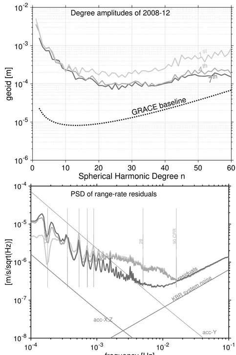
With the goal of understanding these errors, various studies have been carried out in order to investigate the potential of the sensors onboard, their limitations, and the accuracy of the existing background models, even before the launch of the mission. For example, Thomas (1999) studied the potential of the microwave ranging instrument onboard the grace satellites and possible errors (cf. bottom panel of Fig. 1.1). The microwave ranging system uses k- and ka-band frequencies to precisely measure the range and its change between the two satellites. Kim (2000) studied the expected performance of the gravity field solutions computed from grace, prior to its launch. Full-scale simulations were carried out with the aim of computing the expected precision of the time-variable gravity field, under the consideration of expected errors in the range observations. The gravity field computed from those simulations is referred to as the grace baseline. Today, when every data processing center computes a gravity field model from the grace observations, they refer their models to this baseline, shown in top panel of Fig. 1.1.
After the launch of the mission, knowing that the real grace gravity field so- lutions are not as precise as their predicted baseline, numerous studies were pub- lished focusing on:
# understanding the individual error sources and their contribution to the gravity field models,
# improvement of data preprocessing, data and noise modeling approaches.
A selection is listed in Table 1.1 with the description of their focus areas.
These studies certainly improved the knowledge of the noise in the range ob-
servations, data processing and modeling strategies which resulted in an improved
gravity field model (reducing the differences between the baseline and the obtained
gravity field solutions). Since the baseline has not been reached yet, the quest to
Spherical Harmonic Degree n
0 10 20 30 40 50 60
geoid [m]
10-6 10-5 10-4 10-3 10-2
Degree amplitudes of 2008-12
GRACE baseline 1st
4th 7th
frequency [Hz]
10-4 10-3 10-2 10-1
[m/s/sqrt(Hz)]
10-8 10-7 10-6 10-5 10-4
PSD of range-rate residuals
residuals
1 CPR 28 90 CPR
acc-Y acc-X,Z
KBR system noise
Figure 1.1: Top panel: Status of the itsg-2014 solutions as compared to the grace
baseline for december 2008 are shown in terms geoid degree amplitudes. The differ-
ences ( itsg-2014) are plotted with respect to the static field goco 05s. The numbers
1, 4, 7 represent the status of the gravity field solutions computed in an iterative least-
squares approach. Bottom panel: Power Spectral Density (PSD) of postfit range-rate
residuals compared with the available sensor noise models for december 2008 at ev-
ery iteration step of the iterative least-squares parameter estimation approach. CPR
refers to the cycles per revolution.
Table 1.1: Some studies published after the launch of grace with focus on the errors in the gravity field solutions.
Studies by Research Focus
Ko (2008); Ko et al. (2012) KBR microwave ranging system Flury et al. (2008); Hudson (2003); Peter-
seim (2014); Peterseim et al. (2012) GRACE Accelerometer Bandikova et al. (2012); Horwath et al.
(2011); Inácio et al. (2015); Ko and Eanes
(2015) Star camera, inter-satellite pointing
Ditmar et al. (2012) Error in GRACE gravity field models Bonin and Chambers (2011); Chambers
and Bonin (2012) Atmosphere and Ocean De-aliasing er- Han et al. (2004); Knudsen et al. (2001) rors Ocean model errors
investigate the noise in the observations is still ongoing. It is a primary objective to achieve the desired precision of the gravity field solutions. The grace-follow on mission has been launched recently and similar problems might be faced by the science community due to lack of knowledge about the precision of the observations.
Thus, it is an urgent requirement to achieve a better understanding of the noise behavior in the observations in order to fully exploit them to obtain precise gravity field solutions.
The global gravity field parameters are estimated in the least-squares sense where the observation set-up is as follows (Koch, 1990)
l − Aˆ x = e, ˆ 1.3
where l is the vector of the reduced range-rate observations which are computed by
removing all the perturbations mentioned in Eq. 1.2 from the k-band measurements,
A is the design matrix, Aˆ x represents the vector of fitted observations obtained after
estimating the parameters x, and ˆ e ˆ refers to the residuals computed by subtracting
the range-rate observations and the fitted observations. The parameter estimation
approach aims to determine the parameters with the best fit to the original observa-
tions, which means, the residuals ( e ˆ ) must be minimized. Besides being small, the
residuals must be random in nature. That means, they should not be predictable or
correlated with any other variable of the system of equations which would otherwise indicate an insufficiency of the modeling approach. Also, the power spectral density (psd) of the residuals ( e ˆ ) obtained after grace parameter estimation shows that they are larger than the expected sensor noise level (cf. bottom panel of Fig. 1.1).
The expected sensor noise level was predicted by Kim (2000) and has been plotted for the accelerometer (acc) and the k-band ranging (kbr) instrument noise in the bottom panel of Fig. 1.1. Not only the residuals ( e) are large, they also contain ˆ signal characteristics such as 1 cpr (cycles per revolution) or 2 cpr signals which certainly does not represent a random noise behavior.
This work focuses on the characterisation of such behavior of the range-rate resid- uals. Their characterisation is important due to following reasons:
– To understand the deterministic and stochastic behavior of the range-rate residuals. The deterministic characteristics depend on other observations and can be modeled, whereas the stochastic characteristics represent the random behavior, which can not be predicted, and change randomly. Knowing the de- terministic part will be helpful to implement the realistic empirical parameters to be estimated along with the global gravity field parameters. Knowledge of the stochastic part will be helpful in implementing a realistic stochastic noise model.
– The fitted range-rate residuals are used to compute the variance factor which is further used to determine the covariance matrix in the least-squares parameter estimation. The errors in the residuals propagate to the solution via covariance information applied to the observations. Therefore, minimizing the errors in the residuals will reflect an improvement in the precision of the estimated gravity field solutions. It is also shown in Fig. 1.1 where the reduced values of residuals (bottom panel) improve the gravity field solutions (top panel) in an iterative least-squares fit approach. This is only possible by gaining knowledge about the characteristics and behavior of the residuals. A similar study was presented earlier by Ditmar et al. (2006), the authors where they modeled the noise based on frequency-dependent weights of the observations and improved the precision of the gravity field solutions from the observations of champ.
Note that due to the non-linearity of the observation set up, large differences
are seen between the psd of the residuals at 4
thand 7
thiteration in the bottom panel of Fig. 1.1.
– The analysis of the residuals of the observations serves as a quality assessment criteria which presents the quality of the parameters estimated during the least-squares fit. The residuals obtained after the least-squares fit represent an approximation of the true errors in the range-rate observations. Hence, their psd shown in Fig. 1.1 represents an approximation of the true error and can be used to describe the precision of the estimated gravity field solutions. For example, a study by Pail (2004) presented an analysis of the spectral behavior of the gradiometer residuals to assess the quality of gravity field solutions derived in a simulation scenario like goce. They further emphasized the use of residual quantities to identify the outliers, and reducing the residuals by outlier removal, filtering and using those reduced residuals to re-estimate the gravity field parameters iteratively to ultimately obtain an improved gravity field model. Xianping and Yanc-Yuanxi (2005) showed an assessment of the quality of the champ derived gravity field solutions by comparing the fitted residuals computed using two different approaches.
Due to the high relevance of these fitted residuals in determining and assessing the accuracy of estimated gravity field parameters, this study focuses on their de- tailed analysis and gives a comprehensive overview of the systematic errors present in them.
Since the estimated residuals include a portion of the errors and signal which has been partially mapped or aliased into the estimated global gravity field parameters, their analysis can provide a good picture of the errors. However, the residuals alone do not allow us to get an absolute quantification of the errors present in the gravity field solutions. As this study solely addresses the analysis of residuals of grace range-rate observations, an absolute error budget is not presented. However, attempts to quantify the investigated errors have been made and are presented accordingly.
As it has been shown in the bottom panel of Fig. 1.1, the range-rate residuals are
one order of magnitude above the sensor noise level. This shows that the potential
of the grace sensor data has not been fully exploited, yet. There remains room
to understand the limitations from the sensor side. This led to define the focus of the work presented in this thesis which is, analyzing the residuals with focus on the sensor errors’ contribution in them.
1.2 Objectives
The objectives of this thesis are defined as:
Analysis of the range-rate residuals with focus on the attitude errors. The identification of errors is helpful in improving the gravity field modeling pro- cedure:
In the range-rate observations, the attitude errors mostly propogate via the star cameras on the grace satellites. In Chapter 3, the attitude errors present in the residuals due to star camera data are analyzed and discussed. Further, taking advantage of the different reprocessed datasets computed by Klinger and Mayer-Gürr (2014) and Bandikova and Flury (2014), the impact of atti- tude errors on the gravity field solutions are investigated.
Analysis of the range-rate residuals with focus on the kbr instrument noise.
The knowledge of kbr instrument noise is helpful in reducing those errors from the grace gravity field models. It is presented in Chapter 4:
Here, an analysis of the range-rate residuals is presented with focus on the spectra where the kbr instrument noise dominates. The dominating kbr system noise in the range-rate residuals has been studied in detail with the focus on possible error sources. The impact of this noise on the gravity field solutions is also discussed considering various simulation scenarios.
Analysis of the range-rate residuals with focus on the accelerometer errors.
The identified errors coming from the accelerometer are helpful in reducing them during the gravity field modeling:
In Chapter 5, systematic errors of the accelerometers which can be seen in the
residuals are studied. Since the accelerometer errors in the frequency range
0.1 - 0.9 mhz are higher than in the frequency range 1 - 4 mhz, the analysis
considers the two frequency bands separately. In the frequency band 1 - 4 mhz,
the errors of the geophysical background models and star camera errors overlap and are also addressed.
The objectives discussed in this work are based on the grace data analysis of
two years, i.e. 2007 and 2008. During this time period, grace data benefitted from
low impact of solar activity affecting the satellites and their observations (Meyer
et al., 2016). Hence, it serves as a good candidate for the systematic error analysis
of the residuals of the range-rate observations.
Gravity Recovery And Climate Experiment Mis- sion
Experiment Mission
2.1 Introduction
The grace mission was launched on 17 march 2002 from plestesk, russia (Tapley et al., 2004a) and has been decomissioned in october 2017. It was a joint mission between nasa, united states, and dlr, germany. The mission consisted of two satellites following each other. It was operated by german space operations center (gsoc) in darmstadt, germany. It was the first dedicated mission launched to map the global time-variable gravity field of the earth.
The grace mission was launched to an altitude of ≈ 500 km with 220 ± 70 km along track separation between the two satellites. Due to the separation, the trailing satellite passes 28 seconds later over the same area through which the leading passes.
The satellite orbit is inclined with an inclination angle of 89
◦which leads to near- global coverage. It takes about 93 minutes for grace to complete one revolution around the earth, resulting in about 15.5 revolutions per day. The mission was originally planned for a period of mininum 5 years. However, it provided science results until mid-2017, which is more than 15 years. The next mission, grace follow-on (g-fo) has been launched on 22 may 2018 to continue the earth’s gravity field measurements from space.
2.2 Applications
Global gravity field solutions computed from grace have a wide number of
applications, such as in hydrology, in sea level rise studies, understanding the na-
ture of ocean currents and ocean heat storage phenomena. In terrestrial hydrology,
the grace data has been used to determine the regional total water storage con-
tent. The global measurements from grace provide information on seasonal and
inter-annual river basin water storage changes (Rodell and Famiglietti, 2002; Steitz
et al., 2002). Some of the recent and important contributions of grace include the
study of ground water discharge in the states of punjab, rajasthan and delhi, india
(Chinnasamy et al., 2015; Rodell et al., 2009). The california drought has also been studied using grace data (Famiglietti, 2014).
Knowledge about melting of the glaciers is essential to study and keep track of the sea level rise. Since from grace data, the rate of mass change can be derived, one can study the rate of melting of big glaciers, loss of mass of big polar ice sheets and thermospheric effects in the oceans (Hsu and Velicogna, 2017). These factors contribute to the budget of sea level rise which is an important concern today for scientists and society.
GRACE data has been successfully used in oceanographic studies, e.g. Kuo et al.
(2008) studied the ocean currents. Boening et al. (2012); Kanzow et al. (2005);
Landerer et al. (2008) studied temperature-dependent phenomena in the oceans such as el-nino, la-nina and ocean bottom pressure changes. Recently, an achievement has been made by the detection of climate driven polar motion changes by Adhikari and Ivins (2016). Overall, grace being the first satellite-to-satellite tracking mission has been really successful in terms of technology as well as in science applications.
2.3 The GRACE observation system
The grace mission is based on low-low satellite-to-satellite tracking (ll–sst).
This principle uses two satellites following each other while moving around the earth.
The two satellites serve as test masses which are sensitive to the mass distribution and its changes inside and on the surface of the earth. The spatial distribution of mass causes variations in the relative distance between the center of masses (com) of the two satellites. Observing the relative distance requires the establishment of a satellite-to-satellite tracking (sst) technique. Realizing this sst principle needs the knowledge of precise orbit and inter-satellite ranging. These requirements are fulfilled by the grace payload which consisted of (major components):
1. GPS space receiver for orbit determination, 2. Accelerometer (acc),
3. K-band Ranging Microwave Assembly (kbr), 4. Star Camera Assembly (sca).
1. GPS Receiver – The grace gps space receiver was provided by jpl, nasa
(see Fig. 2.1a). The receiver is used for precise orbit determination (pod) with
cm-accuracy, time-tagging of all payload data, and atmospheric and ionospheric profiling. To compute the precise orbit of grace, satellite-to-satellite tracking be- tween the grace and the high-altitude orbiting gps satellites is applied (Flechtner, 2000). The absolute positions of the satellites provided by the gps measurements are also important for gravity field parameter estimation. They are required to geo- reference the kbr observations. In other words, the orbit of the grace satellites, computed from the inter-satellite range (sst) measurements only, suffers a singular- ity problem. The inter-satellite ranges being relative measurements are not sufficient to measure the absolute position of each satellite. This singularity problem is alle- viated by the gps measurements which are necessary to obtain a well-conditioned solution (Kim and Tapley, 2002).
2. Accelerometer – Each grace spacecraft carries an electrostatic 3-axis ac- celerometer at its center of mass which measures the electrostatic force necessary to maintain the accelerometer proof mass motionless with respect to the sensor cage (see Fig. 2.1b). The electrostatic force is proportional to the acceleration of the spacecraft due to non-gravitational forces acting on the satellite, i.e. the atmo- spheric drag, solar radiation pressure and earth’s albedo (Touboul et al., 1999b).
The accelerometers are used in gravity field recovery. The effects of non-gravitational forces, observed by the accelerometer, are reduced from the inter-satellite ranging measurements to isolate the gravity field information. Thus, the accuracy of the accelerometer observations directly affects the recovered gravity field (more details are discussed in the following sections and later in Chapter 5).
3. K-Band Ranging (KBR) Microwave Assembly – The k-band microwave ranging assembly system is the key science instrument of grace which measured the dual one-way range change between both satellites with a precision better than 1
µm/
s. The system uses a single horn antenna for transmission and reception of the dual-band k- (24 ghz) and ka-band (32 ghz) microwave signals. Each satellite transmits carrier phase signals on the two frequencies. The linear combination of the sum of those phase measurements at each frequency gives an ionosphere-corrected measurement of the range between the satellites (Flechtner, 2000; Thomas, 1999).
4. Star Camera Assembly (SCA) – The star camera assembly provided by
denmark technical university consists of two star cameras onboard each spacecraft
(see Fig. 2.1c). These sensors are used for the precise pointing between the two
satellites. The attitude of the satellite is determined from the stars in the field of view of the star camera (Dunn et al., 2002). Once the attitude of a spacecraft is obtained, it is compared with the requirements necessary to maintain the pointing between the two satellites. The attitude is then corrected using the attitude control sensors, i.e. thrusters and magnetic torquer rods.
(a.) GPS receiver (b.) SuperStar Accelerometer (c.) Star Camera Assembly Figure 2.1: GRACE Payload, ©Flechtner (2000)
Figure 2.2: Instrument system of the grace satellites
The twin grace satellites work as a single scientific instrument measuring the
range and its changes between the two satellites (cf. Fig. 2.2). The two spacecraft
transmit and receive the signal through the microwave link. They both have their
own instrument system which are identical in terms of their design. As shown in
Fig. 2.2, the heart of the satellite is the instrument processing unit (ipu) which has
a signal processing unit (spu) as sub-component. The ipu extracts the observables
from the radio frequency links (gps and k-band) and spacecraft attitude from the
images recorded by the star cameras. It digitizes the kbr and gps signals. The
accelerometer data is time-tagged by the ipu and then sent to the on board data
handling (odbh) computer to be telemetered to the ground. Thus, ipu serves as a data interface to odbh (Dunn et al., 2002).
The telemetry data is received on-ground and tagged as level 0 data. This level 0 binary data is converted to the so-called level 1a data readable format. Then, this raw level 1a data is processed to get the level 1b data which is available with the sampling rate shown in table 2.1. The level 1a data sampling rates is 10 hz.
The processed level 1b data, which are used for gravity field recovery, is provided
Table 2.1: The level 1 b datasets along with their sampling rates obtained from the level 1 a datasets. These are used in global gravity field parameter estimation.
Level 1B product Data content sampling frequency
(Hz) K-band ranging data
KBR1B Range, range-rates, light-time and an-
tenna offset corrections 0.2
Accelerometer
ACC1B Linear and angular accelerations 1
Star camera
SCA1B Star camera quaternions 0.2
Reduced dynamic orbit
GNV1B Position and velocity of the spacecraft 0.2
with sampling frequencies of 0.2 hz and 1 hz respectively (see table 2.1). The data processing from level 0 to level 1b is done by the jet propulsion laboratory, nasa, usa. Details of the data processing from level 1a to level 1b are given in Wu et al.
(2006).
2.4 Global gravity field parameter estimation from GRACE observations
The range-rate measurements are the main observables used to estimate the global gravity field parameters. The estimated parameters are the Stokes coefficients which represent the variations in the global gravity field of the earth. Here, first the representation of the global gravity field from the Stokes coefficients is discussed.
Later, the full parameter estimation chain is described which has been used to estimate these Stokes coefficients from the range-rate observations.
2.4.1 Gravity field representation
The gravity field of the earth is represented as an expansion series of harmonic functions which is expressed as (Heiskanen and Moritz, 1967)
V ( r, Θ , λ ) = GM R
X∞ l=0
R r
(l+1)
Xl m=0
C ¯
lmcos mλ + ¯ S
lmsin mλ
P ¯
lm(cos Θ) , 2.1
where G is the gravitational constant, M is the mass of the earth, R is the radius, ( r, Θ , λ ) are the position coordinates at which the gravity field is calculated, P ¯
lmthe normalized legendre functions, C ¯
lmand S ¯
lmare the normalized dimensionless Stokes coefficients, l and m are the degree and order of the expansion series.
In reality, the infinite sum of degrees ( l ) is truncated. In this thesis, the field is truncated to degree and order 60.
2.4.2 Gravity field modeling
A number of methods to compute the global gravity field parameters has been
developed. Some of the important and frequently used approaches are: the Energy
balance approach, the Acceleration approach, the Variational equations approach,
the Celestial mechanics approach. After the launch of the grace mission, data
processing centers started to estimate global gravity field solutions using these ap-
proaches. These gravity field models can be downloaded from: http://icgem.gfz-
potsdam.de/series , an iag service provided by gfz (Barthelmes and Köhler,
2016).
The energy balance approach of recovering the gravity field from inter-satellite range-rate observations was introduced by Jekeli (1999). A simple model was derived on the basis of energy conservation that relates the measured range-rates between two satellites to the gravitational potential difference. For more details, see Jekeli (1999).
The acceleration approach, which is based on newton’s second law of motion, links the acceleration vector to the gradient of the gravitational potential. According to Liu (2008), advantage of the acceleration approach is, the errors due to lineariza- tion are minimized whereas its limitation lies in the amplified noise in the range accelerations which are obtained by double differentiation of the range observations.
The most traditional way of gravity field determination is the variational equations approach, e.g. (Reigber, 1989). It combines the problem of parameter estimation with the dynamic orbit determination. In this approach, the dynamic orbit integra- tion is extended to determine the Stokes coefficients ( C ¯
lm, S ¯
lm). Since the relation between the unknown parameters and the observations is non-linear, it is linearized to solve the problem of parameter estimation. This approach is computationally more challenging as compared to the other two. For details, see Montenbruck and Gill (2000); Tapley et al. (2004b).
A variant of the variational equations approach was further explored by Mayer-Gürr (2006) to recover the global gravity field parameters using short arcs. The approach was first applied to compute champ gravity field solutions using kinematic orbits.
The method was then further extended to compute gravity field solutions from the grace inter-satellite ranging measurements. A series of gravity field models from grace observations has been computed starting from itg
1-gracexx
2(Mayer-Gürr, 2007; Mayer-Gürr et al., 2006) to itsg
3-yyyy
4(Klinger et al., 2016; Mayer-Gürr et al., 2014). Every model is an improved version of the previous one in terms of the estimation scheme, noise modeling, data processing and others.
The grace gravity field solutions and the corresponding range-rate residuals analyzed in this thesis are computed using the groops software. It is a software
1Institute of Theoretical Geodesy
2gravity model number, e.g. 01, 02, etc.
3Institute of Theoretical and Satellite Geodesy
4year
package gravity recovery using object oriented programming software (groops) and was written by Torsten Mayer-Gürr and his colleagues from bonn university, germany. Processing standards of the itsg-2014 global gravity field models are used here (Mayer-Gürr et al., 2014) with the following adaptations:
1. Dynamic orbit integration was adapted to the encke’s orbit integration ap- proach explained by Ellmer and Mayer-Gürr (2016).
2. No k-band antenna offset corrections were estimated. In the standard itsg- 2014 solutions, the k-band antenna offset corrections were estimated once per month. But due to the unreliable characteristics of those estimates, they are not estimated here.
The steps of the itsg-2014 data processing chain are as follows (Mayer-Gürr et al., 2014):
Data preprocessing – The grace level 1b data as mentioned in Table 2.1 are preprocessed to be fed into the dynamic orbit integrator. The preprocessing includes:
• resampling of the star camera data (quaternions) and linear accelerations from the accelerometer. The linear accelerations are resampled from 1 s to 5 s sam- pling rate. The star camera data and the linear accelerations are synchronized.
• rotation of linear accelerations from the science reference frame (srf) to the earth-centered inertial (eci) reference frame using the quaternions (more details are provided in Chapter 3). The quaternions used in the itsg-2014 processing are computed by combining the star camera data and angular ac- celerations from acc1b data using a variance component estimation approach (Klinger and Mayer-Gürr, 2014).
• data synchronization: Synchronization of the orbit (gnv1b) and the linear accelerations along with the resampling of the kinematic orbits at 5 minute sampling rate. The kinematic orbits for grace-a and grace-b are pro- cessed by Zehentner (2016). Both gnv1b orbits are rotated from the earth- centered earth-fixed (ecef) reference frame to the eci reference frame using the iers2010 conventions (Petit and Luzum, 2010) .
Dynamic orbit integration – The orbit for each satellite is integrated using
encke’s orbit integration approach (Ellmer and Mayer-Gürr, 2016). The 24 hours
dynamic arc is computed by integrating all forces perturbing the orbit using a poly- nomial approach. The perturbing forces include gravitational and non-gravitational forces as mentioned in the Table 2.2. The integrated orbit is fitted to the kinematic Table 2.2: List of perturbation forces and their models which are applied during orbit integration.
Forces Models
Earth rotation IERS 2010 (Petit and Luzum, 2010)
Direct tides (Moon, Sun and planets) JPL DE421 (Folkner et al., 2009) Solid earth tides IERS 2010 (Petit and Luzum, 2010)
Ocean tides EOT11a (Savcenko and Bosch, 2012)
Pole tides IERS 2010 (Petit and Luzum, 2010)
Ocean pole tides Desai 2003 (Petit and Luzum, 2010)
Atmospheric tides (S1, S2) Bode-Biancale 2003 (Bode and Biancale, 2006) Atmosphere and Ocean Dealiasing AOD1B RL05 (Flechtner et al., 2015)
Relativistic corrections IERS 2010 (Petit and Luzum, 2010)
Permanent tidal deformation includes (zero tide) (Petit and Luzum, 2010) Non conservative forces Accelerometer
orbits. Then this fitted orbit is used as a taylor point for further iterations. The differences between the coordinates of the successive iterations are used to assess the quality of the integrated orbit. After a few iterations, the difference between the two integrated orbits converges to the machine precision (typically within micro meters).
Parameter estimation – A schematic view for solving the problem of global gravity field parameter estimation based on the approach of Mayer-Gürr (2006) is shown in Fig. 2.3. The observation equation in Fig. 2.3 (b.) is a linearized overde- termined system of equations which are solved using the least-squares approach.
The least-squares variance component estimation is used for the recovery of global gravity field parameters (Koch, 1990; Koch and Kusche, 2002).
In Fig. 2.3 (a.), the observation vector l of size ( n ×
1) contains the pre-fit range-rate residuals along with the orbit parameters ( r and ˙r ) and the accelerometer scale and bias parameters. The pre-fit range-rate residuals are computed as:
l
n×1= ( ˙ ρ
KBR− ρ ˙
0)
n×1, 2.2
KBR1B ACC1B SCA1B AOD1B GNV1B
l = Aˆx+ ˆe
ˆ xi=
ATPiA−1
ATPil ˆli = Aˆxi
ˆ
ei = l−ˆli
σ2i = eˆTiPieˆi n−m
(σ2i≈1)ORi= 7 ˆli+1= ˆei
Pi+1=σ2iPi
ˆl=Aˆx ˆ e=l−ˆl
no yes
a.) Input datasets
b.) Observation equation
c.) Parameter estimation
d.) min. square sum of residuals
e.) Output
Figure 2.3: Diagrammatic representation of the chain followed for global gravity field parameter estimation from grace observations.
where ρ ˙
0contains the reduced range-rate observations computed from the integrated dynamic orbit. In Fig. 2.3 (b.), A
(m×n)is the information matrix (also called as design matrix), x ˆ
(n×1)is the vector of parameters to be estimated (cf. Eq. 2.3) and ˆ
e
(m×1)contains the noise in the orbit and the range-rate observations,
ˆ x
i=
C
nm, S
nmorbit parameters ( r, r ˙ ) accelerometer scale and bias
, 2.3
ˆ e
i=
range-rate residuals orbit residuals
. 2.4
The estimation of x ˆ is a correction to the a-priori solution. It is obtained in the
normal equations approach as shown in Fig. 2.3(c.). This system of equations is
solved using an iterative least-squares variance component estimation approach with
an arc-length of 3 hours for each day. The cholesky decomposition method is used to
solve for the system of normal equations and the covariance matrix in order to reduce
the computational costs. In order to minimize the noise from the observations, a
weight matrix ( P ) (cf. Fig. 2.3 (c.)) is introduced in which relative weights are
assigned on the basis of the noise content of the observations. The weight matrix is
Figure 2.4: A schematic flow of the computation of the covariance matrix in ITSG- 2014 model from the esti- mated residuals in an iter- ative least-squares variance component estimation ap- proach, after Mayer-Gürr (2015).
computed from the covariance information of the noise in the observations. Thus, it is also called as the covariance matrix. In the itsg-2014 gravity field solutions, the covariance matrix
Σ
is estimated on the basis of a noise model described by the observation noise in the frequency domain as
Σ = a
12F
1+ a
22F
2+ · · · + a
N2F
N, where , F
N=
cos
2
π
T n ( t
i− t
k)
. 2.5
In the Eq. 2.5, a
12· · · a
N2are the amplitudes of n frequencies, ( t
i− t
k) are the differences between two adjacent time epochs.
The noise information is taken from the set of residuals ( e ˆ
i) obtained after each fit
as shown in Fig. 2.3 (c.). The content of the residual vector is given in Eq. 2.4.
During each iteration, the noise covariance information is computed from the resid- uals of the fitted observations in the frequency domain. The covariance matrix is updated with that information where Σ
0is initialised as an identity matrix (cf. Fig.
2.4) (Mayer-Gürr, 2015). This approach helps to improve x ˆ as observations are weighted according to their accuracy (in frequency domain). After the full param- eter estimation, the estimated unknown parameters, i.e. x ˆ , are obtained (cf. Eq.
2.3).
Although the set of residuals ˆ e contain orbit and range-rate residuals (cf. Eq.
2.4) the range-rate residuals are referred to as ˆ e in the rest of the work for the ease of the reader. It is also because the analysis of other sets of residuals is out of the scope of this work. Since the range-rate residuals analyzed in this work are computed after full parameter estimation, they are referred to as post-fit range-rate residuals, also in short postfits or post-fit residuals.
As shown in Fig. 1.1, the power spectral density (psd) of the range-rate residuals should be at the level of the predicted sensor noise. In the current scenario, there is still a gap of one order of magnitude between the psd of the expected sensor noise and the obtained range-rate residuals. At the same time, it is easily visible that the psd of the range-rate residuals contains typical signal type characteristics (ex- ample 1, 2, ... cpr). This clearly indicates the insufficiency of the current modeling approach which is not fully able to exploit the grace measurement accuracy. It also indicates that the residuals may contain some noise which is predictable, i.e., it is not just random. As mentioned previously, the gap in the psd of the range-rate residuals and the expected sensor noise also indicate that the potential of the sensors is not fully exploited yet and thus, it could be one of the factors limiting the accuracy of the gravity field solution. When the estimated solutions are compared with the anticipated grace accuracy baseline, the existing gap between the two curves make this implication even stronger (cf. top panel of Fig. 1.1). Therefore, a good under- standing of the noise characteristics from all input data is essential to understand the reasons behind the limitations in the accuracy of the grace solutions.
In the following chapters, noise in the three main input datasets will be discussed
i.e., star cameras, accelerometer and k-band microwave ranging measurements along
with their error contribution in the range-rate residuals.
2.5 Analysis kit used for studying the residuals
In this thesis, an analysis of the post-fit range-rate residuals is carried out in the following chapters. These residuals are computed after estimating the global gravity field parameters using the itsg-2014 processing chain described in the previous sections. In the following subsections, the methods and representations used to study the error characteristics of the observations and the error analysis of the gravity field solutions are introduced.
2.5.1 Degree amplitudes
The errors of the recovered global gravity field spherical harmonic coefficients is determined as their 1-d spectra. The error degree variances are given as (Kaula, 1967; Sneeuw, 2000)
σ
l2=
Xlm=0
( C
lm2+ S
lm2) , 2.6 where l, m are the degree and order of the Stokes coefficients or spherical harmonic coefficients. Eq. 2.6 represents the total signal power of the coefficients. In this thesis, results are investigated for the parameters estimated up to degree and order 60. The investigated results are represented as the geoid degree amplitudes which is obtained as
q
σ
l2× R, 2.7
where R is the radius of the earth which is 6.378136 × 10
6meters.
A representation of geoid amplitudes vs degree for example is shown in top panel of Fig. 1.1 of Chapter 1.
2.5.2 Power Spectral Density (PSD)
It describes how the power of a time-series is distributed with frequency. A psd
is also defined as the fourier transform of the autocorrelation sequence of a time-
series (Heinzel et al., 2002). A PSD of a time-series y ( t ), where t is the time, is
defined as
φ ( ω ) =
X∞ k=−∞
r ( k ) e
−iωk, 2.8
where ω =
2πf , f is frequency.
r ( k ) is the autocovariance sequence given as
r ( k ) = E { y ( t ) y
∗( t − k )} , 2.9 where E is the expectation operator and k represents the lag factor which is 0 for the autocovariance function.
PSDs of the continuous segments of the satellite observations are computed using the
“lpsd” method provided in the ltpda toolbox (Hewitson, 2007). For example, the psd of residuals is shown in the bottom panel of Fig. 1.1. In all cases, a Hanning Window has been used with 50 % overlap with a peak sidelobe level
1(psll) of 31.5 db. More details about the implementation of the “lpsd” method are provided in Heinzel et al. (2002).
2.5.3 Time-series analysis
The time-series representation gives the observations (on y-axis) and their vari- ations with respect to time (on x-axis) (for example, Fig. 4.3). It is helpful for understanding the variations in the characteristics of the satellite observations with respect to time such as the systematics related to the satellite-orbit maneuvers.
For the statistical analysis of the time-series, the correlations are also exploited further. The correlation coefficients of two random variables define the linear de- pendence between them. The Pearson correlation coefficient used in this work is
1The window function in the frequency domain contains the central peak which is the desired one alongwith many side peaks at regular intervals. These side peaks are called ‘sidelobes’. The aim is to reduce the amplitude of these sidelobes without widening the noise bandwidth. The widening of the noise bandwidth causes spectral leakage. Hence, a compromise between the sidelobe level and the noise bandwidth is important in designing the window function (Heinzel et al.,2002).
computed as (Press et al., 1992)
ρ ( A, B ) = cov ( A, B )
σ
Aσ
B, where 2.10
cov ( A, B ) =
1N −
1XN i=1