2 Parity Games and Fixed-Point

(1)

Logic and Games WS 2015/2016

Prof. Dr. Erich Grädel

Notes and Revisions by Matthias Voit

Mathematische Grundlagen der Informatik RWTH Aachen

(2)

c b n d

This work is licensed under:

http://creativecommons.org/licenses/by-nc-nd/3.0/de/

Dieses Werk ist lizenziert unter:

http://creativecommons.org/licenses/by-nc-nd/3.0/de/

http://www.logic.rwth-aachen.de

2 Parity Games and Fixed-Point

Logics

In the first chapter we have discussed model checking games for first- order logic and modal logic. These games admit only finite plays and their winning conditions are specified just by sets of positions, that the players want to reach. Winning regions in these games can be computed in linear time with respect to the size of the game graph.

However, in many computer science applications, more expressive logics are needed, such as temporal logics, dynamic logics, fixed-point logics and others. Model checking games for these logics admit infinite plays and their winning conditions must be specified in a more elaborate way. As a consequence, we have to consider the theory of infinite games.

For fixed-point logics, such as LFP or the modalµ-calculus, the appropriate evaluation games areparity games. These are games of possibly infinite duration with a function that assigns to each position a natural number, called itspriority. The winner of an infinite play is determined according to whether the least priority seen infinitely often during the play is even or odd.

2.1 Parity Games

Definition 2.1. Aparity gameis given by a labelled game graphG = (V,V₀,V₁,E,Ω)as in Sect. 1.3 with a functionΩ:V→^Nthat assigns a priorityto each position. The setVof positions may be finite or infinite, but|Ω(V)|, the number of different priorities which is called theindex ofG, must be finite. As before, a finite play is lost by the player who gets stuck, i.e. cannot move. For infinite playsv0v1v2. . ., we have the parity winning condition: If the least number appearing infinitely often in

(4)

2 Parity Games and Fixed-Point Logics

the sequenceΩ(v0)Ω(v1). . . of priorities is even, then Player 0 wins the play, otherwise Player 1 wins.

A strategy (for Playerσ) is a function f : V^∗Vσ → V such that f(v₀v₁. . .vn)∈vnE. We say that a playπ=v₀v₁. . . isconsistentwith the strategy fof Playerσif for eachvi∈Vσit holds thatvi+1= f(v0. . .vi). The strategyfiswinningfor Playerσfrom (or on) a setW⊆Vif each play starting inWthat is consistent with fis won by Playerσ.

In general, a strategy may depend on the entire history played so far, and can thus be a very complicated object. However, we are interested in simple strategies that depend only on the current position.

Definition 2.2. A strategy (of Playerσ) is calledpositional(ormemoryless) if it only depends on the current position, but not on the history of the play, which means thatf(hv) = f(h^′v)for allh,h^′∈V^∗,v∈V. We can view positional strategies simply as functionsf :Vσ→V.

We shall see that positional strategies suffice to solve parity games.

Before we formulate and prove this Forgetful Determinacy Theorem, we recall that positional strategies are of course sufficient whenever, as in the previous chapter, the players have purely positional objectives such as reachability or safety. Specifically, for every gameG= (V,V₀,V₁,E) and everyX⊆Vwe have defined the attractor

Attrσ(X) ={v∈V: Playerσhas a strategy fromvto reach some positionx∈X∪Tσ}

and such anattractor strategycan, without loss of generality, assumed to be positional. Similarly, ifY ⊆Vis atrapfor Playerσ, then Player (1−σ)has a positionaltrap strategyto keep the play insideY.

Further we note that positional winning strategies on parts of the game graph may be combined to positional winning strategies on larger regions. Indeed, let fandf^′be positional strategies for Playerσthat are winning on the setsW,W^′, respectively. Let(f+f^′)be the positional strategy defined by

2.1 Parity Games

(f+f^′)(x):=





f(x) ifx∈W f^′(x) otherwise.

Then(f+f^′)is a winning strategy onW∪W^′.

We can now turn to the proof of the Forgetful Determinacy Theorem.

Theorem 2.3(Forgetful Determinacy). In any parity game, the set of positions can be partitioned into two setsW0andW1such that Player 0 has a positional strategy that is winning on W₀ and Player 1 has a positional strategy that is winning onW1.

Proof. Let G = (V,V0,V1,E,Ω) be a parity game with |Ω(V)| = m.

Without loss of generality we can assume thatΩ(V) ={0, . . . ,m−1}or Ω(V) ={1, . . . ,m}. We prove the statement by induction over|Ω(V)|.

In the case that|Ω(V)|=1, i.e.,Ω(V) ={0}orΩ(V) ={1}, either Player 0 or Player 1 wins every infinite play. Her opponent can only win by reaching a terminal position that does not belong to him. So we have, forΩ(V) ={σ},

W1−σ=Attr_1−σ(T1−σ)and Wσ =V\W1−σ.

ComputingW1−σas the attractor ofT1−σis a simple reachability problem, and thus it can be solved with a positional strategy. ForWσthere is a positional strategy that avoids leaving this (1−σ)-trap.

Let now|Ω(v)| = m > 1. We explicitly consider the case that 0 ∈ Ω(V), i.e., Ω(V) = {0, . . . ,m−1}. Otherwise, if the minimal priority is 1, we can use the same argumentation with switched roles of the players. We define

X1:={v∈V: Player 1 has a positional winning strategy fromv}, and letgbe a positional winning strategy for Player 1 onX1.

Our goal is to provide a positional winning strategyf^∗for Player 0 onX0:=V\X1, so in particular we haveW1=X1andW0=V\X1.

First of all, observe thatX0is a trap for Player 1. Indeed, if Player 1 could reach X1 from somev ∈ X0, then Player 1 could win with a

(5)

positional strategy fromv, sovwould also be inX1. Thus, there exists a positionaltrap strategy tfor Player 0 onX₀that guarantees that a play remains insideX0.

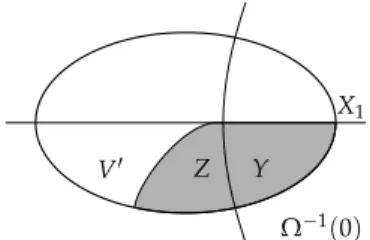
LetY = Ω⁻¹(0)∩X0andZ = Attr0(Y). Player 0 has positional attractor strategyato ensure, from every positionz∈Z\Y, thatY(or a terminal winning position inT0) is reached in finitely many steps.

Let nowV^′ = V\(X1∪Z). The restricted game G^′ = G|V^′ has strictly fewer priorities thanG(since at least all positions with priority 0 have been removed). Thus, by induction hypothesis, the Forgetful Determinacy Theorem holds forG^′. This means thatV^′=W₀^′∪W₁^′and there exist positional winning strategies f^′for Player 0 onW₀^′andg^′for Player 1 onW₁^′inG^′.

However, it follows thatW₁^′=∅, since the strategy

(g+g^′):x7→





g(x) x∈X1

g^′(x) x∈W₁^′

is a positional winning strategy for Player 1 onX1∪W₁^′. Indeed, every play consistent with(g+g^′)either stays inW₁^′and is consistent with g^′or reachesX₁^′and is from this point on consistent withg. ButX1, by definition, already containsallpositions from which Player 1 can win with a positional strategy, soW₁^′=∅.

X1

V^′ Z Y

Ω⁻¹(0)

Figure 2.1.Construction of a winning strategy

Knowing thatW₁^′=∅, letf^∗= f^′+a+t, i.e.

2.1 Parity Games

f^∗(x) =











f^′(x) ifx∈W₀^′ a(x) ifx∈Z\Y t(x) ifx∈Y

We claim that f^∗is a positional winning strategy for Player 0 fromX0. Note that ifπis a play that is consistent withf^∗, thenπremains inside X0. We distinguish two cases.

Case (a): πhitsZonly finitely often. Thenπeventually stays inW₀^′and is consistent withf^′from this point onwards. Hence Player 0 winsπ.

Case (b): πhitsZ infinitely often. Thenπalso hitsY infinitely often, which implies that priority 0 is seen infinitely often. Thus, Player 0

winsπ. q.e.d.

The following theorem is a consequence of positional determinacy.

Theorem 2.4.It can be decided in NP∩coNP whether a given position in a parity game is a winning position for Player 0.

Proof. A node vin a parity game G = (V,V0,V1,E,Ω)is a winning position for Playerσ if there exists a positional strategy f : Vσ → V which is winning from positionv. It therefore suffices to show that the question whether a given strategy f:Vσ→Vis a winning strategy for Playerσfrom positionvcan be decided in polynomial time. We prove this for Player 0; the argument for Player 1 is analogous.

GivenGand f :V0→V, we obtain a reduced game graphGf = (W,F)by retaining only those moves that are consistent with f, i.e.,

F={(v,w):(v∈W∩Vσ∧w=f(v))∨ (v∈W∩V1−σ∧(v,w)∈E)}.

In this reduced game, only the opponent, Player 1, makes non-trivial moves. We call a cycle in(W,F)odd if the least priority of its nodes is odd. Clearly, Player 0 winsGfrom positionvvia strategy fif, and only if, inGfno odd cycle and no terminal positionw∈V0is reachable fromv. Since the reachability problem is solvable in polynomial time,

the claim follows. q.e.d.

(6)

2.2 Algorithms for parity games

It is an open question whether winning sets and winning strategies for parity games can be computed in polynomial time. The best algorithms known today are polynomial in the size of the game, but exponential with respect to the number of priorities. On an class of parity games with bounded index, such algorithms run in polynomial time.

One way to intuitively understand an algorithm solving a parity game is to imagine a referee who watches the players playing the game.

At some point, the referee is supposed to say “Player 0 wins”, and indeed, whenever the referee does so, there should be no question that Player 0 wins. We shall first give a formal definition of a certain kind of referee with bounded memory, and later use this notion to construct algorithms for parity games.

Definition 2.5. A referee M = (M,m0,δ,F) for a parity game G = (V,V0,V1,E,Ω)consists of a set of statesMwith a distinguished initial statem0 ∈ M, a set of final states F ⊆ M, and a transition function δ : V×M→M. Note that a referee is thus formally the same as an automaton reading words over the alphabetV. But to be called a referee, two further conditions must be satisfied, for any playv0v1. . . ofG, and and the corresponding sequencem₀m₁. . . of states ofM, wherem₀is the initial state ofMandmi+1=δ(vi,mi):

(1) Ifv0. . . is winning for Player 0, then there is aksuch thatm_k∈F, (2) Ifmk∈Ffor somek, then there existi<j≤ksuch thatvi=vjand

min{Ω(vi+1),Ω(vi+2), . . . ,Ω(vj)}is even.

To illustrate the second condition in the above definition, note that in the playv0v1. . . the sequencevivi+1. . .vjforms a cycle. Assuming that both players use a positional strategy the decision of the referee is correct. Indeed, if a cycle with even priority appears, then this cycle will be repeated forever, Player 0 can be declared as the winner. To capture this intuition formally, we define the following reachability game, which emerges as the product of the original gameGand the refereeM. Definition 2.6. LetG = (V,V0,V1,E,Ω)be a parity game and M = (M,m0,δ,F)an automaton reading words overV. We associate withG

2.2 Algorithms for parity games

andMa reachability game

G × M= (V×M,V0×M,V1×M,E^′,V×F),

where((v,m), (v^′,m^′))∈E^′iff(v,v^′)∈Eandm^′=δ(v,m), andV×F is the set of positions which are immediately winning for Player 0 (the goal of Player 0 is to reach such a position). Plays that do not reach a position inV×Fare won by Player 1.

Note thatMin the definition above is a deterministic automaton, i.e.,δis a function. Therefore, inGand inG × Mthe players have the same choices, and thus it is possible to translate strategies betweenG andG × M. Formally, for a strategyfinGwe define the strategyfin G × Mas

f((v0,m0)(v1,m1). . .(vn,mn)) = (f(v0v1. . .vn),δ(vn,mn)). Conversely, given a strategy finG × Mwe define the strategy finG such thatf(v0v1. . .vn) =vn+1if and only if

f((v0,m0)(v1,m1). . .(vn,mn)) = (vn+1,mn+1),

wherem0m1. . . is the unique sequence corresponding tov0v1. . ..

WithG × Mwe are ready to prove that the definition of a referee indeed makes sense for parity games.

Theorem 2.7. Let G be a parity game andMa referee for G. Then Player 0 winsGfromv₀if, and only if, she winsG × Mfrom(v₀,m₀). Proof. (⇒) Letfbe a winning strategy for Player 0 inGfromv0. Assume that Player 0 does not have a winning strategy forG × Mfrom(v0,m0). By determinacy of reachability games, there exists a winning strategyg for Player 1. Consider the unique playπ_G=v0v1. . . that is consistent with fandgand the unique playπ_G×M= (v₀,m₀)(v₁,m₁). . . which is consistent withf andg. Observe that the positions ofGappearing in both plays are indeed the same due to the wayfandgare defined.

Since Player 0 winsπ_G, by Property (1) in the definition of a referee there must be anmk∈F. But this contradicts the fact that Player 1 wins π_G×M.

(7)

(⇐) Letf be a winning strategy for Player 0 inG × M, and assume that Player 1 has apositionalwinning strategyginG. Again, we consider the unique playspi_G =v0v1. . . andπ_G×M= (v0,m0)(v1,m1). . . such thatπ_Gis consistent withfandg, andπ_G×Mis consistent withfand g. Sinceπ_G×Mis won by Player 0, there is anmk∈Fappearing in this play.

By Property (2) in the definition of a referee, there exist two indices i<jsuch thatvi=vjand the minimum priority appearing betweenvi

andvjis even. Let us now consider the following strategyf^′for Player 0 inG:

f^′(w0w1. . .wn) =





f(w0w1. . .wn) ifn<j, f(w0w1. . .wm) otherwise,

wherem=i+ [(n−i) mod(j−i)]. Intuitively, the strategy f^′makes the same choices as f up to the(j−1)st step, and then repeats the choices of ffrom stepsi,i+1, . . . ,j−1.

We claim that the unique playπ^′inGthat is consistent with both f^′andgis won by Player 0. Since in the firstjstepsf^′is the same as f, we have thatπ[n] =vnfor alln≤j. Now observe thatπ[j+1] =vi+1. Sincegis positional, ifvjis a position of Player 1, thenπ[j+1] =vi+1, and ifv_jis a position of Player 0, thenπ[j+1] =v_i+1because we defined f^′(v0. . .vj) =f(v0. . .vi). By induction we get that the playπrepeats the cyclevivi+1. . .vjinfinitely often, i.e.

π=v0. . .vi−1(vivi+1. . .vj−1)^ω.

Thus, the minimal priority occurring infinitely often inπis the same as min{Ω(v_i),Ω(v_i+1), . . .Ω(v_j−1)}, and thus is even. Therefore Player 0 winsπ, which contradicts the fact thatg was a winning strategy for

Player 1. q.e.d.

This theorem allows us, if a referee is known, to reduce the problem of solving a parity game to the problem of solving a reachability game, which we already tackled with the Gamealgorithm. But to make use of it, we first need to construct a referee for a given parity game.

2.2 Algorithms for parity games The most naïve way to build a referee for a parity game is to just remember, for each positionv visited during the play, the minimal priority seen since the last occurrence ofv. If it happens that a position vis repeated, and the minimal priority seen since the last occurrence of vis even, the referee decides that Player 0 wins the play.

It is easy to check that an automaton defined in this way is indeed a referee forG, but such a referee can be very big. Since for each of the

|V|=npositions we need to store one of|Ω(V)|=dcolours, the size of the referee is in the order ofO(dⁿ). We shall present a referee that is much better for smalld.

Definition 2.8. Aprogress-measuring refereeMP = (MP,m0,δP,FP)for a parity gameG = (V,V0,V1,E,Ω)is constructed as follows. Ifn_i=

|Ω⁻¹(i)|is the number of positions with priorityi, then

MP={0, 1, . . . ,n0+1} × {0} × {0, 1, . . . ,n2+1} × {0} ×. . . and this product ends in· · · × {0, 1, . . . ,nm+1}if the maximal priority mis even, or in· · · × {0}if it is odd. The initial state ism0= (0, . . . , 0), and the transition functionδ(v,c)withc= (c0, 0,c2, 0, . . . ,cm)is given by

δ(v,c) =





(c0, 0,c2, 0, . . . ,c_Ω(v)+1, 0, . . . , 0) ifΩ(v)is even, (c0, 0,c2, 0, . . . ,c_Ω(v)₋₁, 0, 0, . . . , 0) otherwise.

The setF_Pcontains all tuples(c0, 0,c2, . . . ,cm)in which some counter cj=nj+1 reached the maximum possible value.

The intuition behindMPis that it counts, for each even priorityp, how many positions with prioritypwere seen without any lower priority in between. If more thannpsuch positions are seen, then at least one must have been repeated, which guarantees thatMPis a referee.

Lemma 2.9. For each finite parity gameG the automaton MP constructed above is a referee forG.

Proof. We need to show thatMPexhibits the two properties characteris- ing a referee:

(8)

(1) ifv0. . . is winning for Player 0, then there is aksuch thatm_k∈F, (2) if, for somek,mk∈F, then there existi<j≤ksuch thatvi=vj

and min{Ω(vi+1),Ω(vi+2), . . . ,Ω(v_j)}is even.

To see (1), assume thatv0v1. . . is a play winning for Player 0. Let k be such an index that Ω(v_k) is even, appears infinitely often in Ω(vk)Ω(vk+1). . ., and no priority higher thanΩ(vk)appears in this play suffix. Then, starting from v_k, the counterc_Ω(v_k₎ will never be decremented, but it will be incremented infinitely often. Thus, for a finite gameG, it will reachn_Ω(v_k)+1 at some point, i.e. a state inFP.

To prove (2), letv0v1. . .vkbe such a prefix of a play that aftervk

some countercpis set tonp+1 for an even priorityp. Letv_i₀be the last position at which this counter was 0, andvimthe subsequent positions at which it was incremented, up toinp=k. All positionsvi0,vi1, . . . ,vi_np

have priority p, but since there are onlynp different positions with priorityp, we get that, for somek<l,vik =vil. Nowikandilare the positions required to witness (2), because indeed the minimum priority betweeni_kandi_lispsincecpwas not reset in between. q.e.d.

For a parity gameGwith an even number of prioritiesd, the above presented referee has sizen0·n2· · ·nd, which is at most(_d/2ⁿ )^d/2. We get the following corollary.

Corollary 2.10. Parity games can be solved in timeO((_d/2ⁿ )^d/2).

Notice that the algorithm using a referee has high space demand:

Since the product gameG × MPmust be explicitly constructed, the space complexity of this algorithm is the same as its time complexity. There is a method to improve the space complexity by storing the maximal counters the refereeMPuses in each position and lifting such annotations. This method is calledgame progress measuresfor parity games. We will not define it here, but the equivalence to modalµ-calculus proven in the next chapter will provide another algorithm for solving parity games with polynomial space complexity.

2.3 Fixed-Point Logics

We will define two fixed-point logics, the modalµ-calculus, Lµ, and the first-order least fixed-point logic, LFP, which extend modal logic and first-order logic, respectively, with the operators for least and greatest fixed-points.

The syntax of Lµis analogous to modal logic, with two additional rules for building least and greatest fixed-point formulas:

µX.φ(X)andνX.φ(X)

are Lµformulas ifφ(X)is, whereXis a variable that can be used inφ the same way as predicates are used, but mustoccur positively inφ, i.e.

under an even number of negations (or, ifφis in negation normal form, simply non-negated).

The syntax of LFP is analogous to first-order logic, again with two additional rules for building fixed-points, which are now syntactically more elaborate. Letφ(T,x₁,x₂, . . .xn)be a LFP formula whereTstands for ann-ary relation and occurs only positively inφ. Then both

[lfpTx.φ¯ (T, ¯x)](a¯)and[gfpTx.φ¯ (T, ¯x)](a¯) are LFP formulas, wherea=a1. . .an.

To define the semantics of Lµand LFP, observe that each formula φ(X)of Lµorφ(T, ¯x)of LFP defines an operatorJφ(X)_K : P(V)→ P(V)on statesVof a Kripke structureKandJφ(T, ¯x)_K : P(Aⁿ)→ P(Aⁿ) on tuples from the universe of a structureA. The operators are defined in the natural way, mapping a set (or relation) to a set or relation of all these elements, which satisfyφwith the former set taken as argument:

Jφ(X)K(B) ={v∈ K:K,v|=φ(B)}, and Jφ(T, ¯x)_K(R) ={a¯∈A:A|=φ(R, ¯a)}.

An argumentBis a fixed-point of an operator f if f(X) = X, and to complete the definition of the semantics, we say thatµX.φ(X)defines

(9)

thesmallestsetBthat is a fixed-point ofJφ(X)K, andνX.φ(X)defines the largestsuch set. Analogously,[lfpTx.φ¯ (T, ¯x)](x¯)and[gfpTx.φ¯ (T, ¯x)](x¯) define the smallest and largest relations being a fixed-point ofJφ(T, ¯x)K, respectively. In a few paragraphs, we will give an alternative characteri- sation of least and greatest fixed-points, which is better tailored towards an algorithmic computation.

To justify this definition, we have to assure that all notions are well- defined, i.e., in particular, we have to show that the operators actually have fixed-points, and that least and greatest fixed-points always exist.

In fact, this relies on the monotonicity of the operators used.

Definition 2.11.An operatorFismonotoneif X⊆Y =⇒ F(X)⊆F(Y).

The operatorsJφ(X)_KandJφ(T, ¯x)_Kare monotone because we assumed thatX(orT) occurs only positively inφ, and, except for negation, all other logical operators are monotone (the fixed-point operators as well, as we will see). Each monotone operator not only has unique least and greatest fixed-points, but these can be calculated iteratively, as stated in the following theorem.

Remark2.12. A formal definiton of ordinal numbers can be found in appendix A. For the moment, we think of them as a generalisation of the naturals numbers which allow to count beyond the finite. The first ordinal numbers are the natural numbers 0, 1, 2, . . . itself. The least infinite ordinal number is the set of all natural numbers, written asω, followed byω+1,ω+2, . . . ,ω·2,ω·2+1, . . . ,ω², . . . ,ω^ω, . . ..

Definition 2.13.LetAbe a set, andF:P(A^k)→ P(A^k)be a monotone operator. We define the stagesXαof an inductive fixed-point process:

X0:=∅ Xα+1:= f(Xα)

X_λ:= ^[

α<λ

Xα for limit ordinalsλ.

Due to the monotonicity ofF, the sequence of stages is increasing, i.e.

2.4 Model Checking Games for Fixed-Point Logics Xα ⊆ Xβ forα< β, and hence for someγ, called theclosure ordinal, we haveXγ=X_γ+1=F(Xγ). This fixed-point is called theinductive fixed-pointand denoted byX∞.

Analogously, we can define the stages of a similar process:

X⁰:=A^k X^α+1:=F(X^α)

X^λ:= ^\

α<λ

X^α for limit ordinalsλ.

which yields a decreasing sequence of stagesX^αthat leads to the inductive fixed-pointX^∞:=X^γfor the smallestγsuch thatX^γ=X^γ+1. Theorem 2.14(Knaster, Tarski). Let Fbe a monotone operator. Then the least fixed-point lfp(F) and the greatest fixed-point gfp(F) of F exist, they are unique and correspond to the inductive fixed-points, i.e.

lfp(F) =X∞, and gfp(F) =X^∞.

To understand the inductive evaluation let us consider an example.

We will evaluate the formulaµX.(P∨♢X) on the following Kripke structure:

K= ({0, . . . ,n},{(i,i+1)|i<n},{n}).

The structureKrepresents a path of lengthn+1 ending in a position marked by the predicate P. The evaluation of this least fixed-point formula starts withX0= ∅andX1= P={n}, and in stepi+1 all nodes having a successor inX_iare added. Therefore,X2={n−1,n}, X3={n−2,n−1,n}, and in generalXk={n−k+1, . . . ,n}. Finally, Xn+1=Xn+2={0, . . . ,n}. As you can see, the formulaµX.(P∨♢^X) describes the set of nodes from whichPis reachable. This example shows one motivation for the study of fixed-point logics: It is possible to express transitive closures of various relations in such logics.

2.4 Model Checking Games for Fixed-Point Logics

In this section we will see that parity games are the model checking games for LFP and Lµ.

(10)

We will construct a parity gameG(A,Ψ(a¯))from a formulaΨ(x¯)∈ LFP, a structureAand a tuple ¯aby extending the FO game with the moves

[fpTx.φ¯ (T, ¯x)](a¯)→φ(T, ¯a) and

Tb¯→φ(T, ¯b).

We assign prioritiesΩ(φ(a¯))∈^Nto every instantiation of a subformula φ(x¯). Therefore, we need to make some assumptions onΨ:

•Ψis given in negation normal form, i.e. negations occur only in front of atoms.

• Every fixed-point variable T is bound only once in a formula [fpTx.φ¯ (T, ¯x)].

• In a formula[fpTx.φ¯ (T, ¯x)]there are no other free variables besides x¯inφ.

Then we can assign the priorities using the following schema:

•Ω(T¯a)is even ifTis a gfp-variable, andΩ(T¯a)is odd ifTis an lfp-variable.

• IfT^′depends onT(i.e. Toccurs freely in[fpT^′x.φ¯ (T,T^′, ¯x)]), then Ω(T¯a)≤Ω(T^′b¯)for all ¯a, ¯b.

•Ω(φ(a¯))is maximal ifφ(a¯)is not of the formTa.¯

Remark2.15. The minimal number of different priorities in the game G(A,Ψ(a¯))corresponds to the alternation depth ofΨ.

Before we provide the proof that parity games are in fact the appropriate model checking games for LFP and Lµ, we introduce the notion of anunfoldingof a parity game.

Let G = (V,V0,V1,E,Ω)be a parity game. We assume that the minimal priority inGis 0 and that all positionsv∈VwithΩ(v) =0 have a unique successor, i.e.,vE={s(v)}.

LetT={v ∈V :Ω(v) = 0}. We define a modified gameG⁻ = (V,V0,V1,E⁻,Ω)withE⁻=E\(T×V), i.e., positions inTare made terminal positions inG⁻. Further, we define a sequence of gamesG^αthat only differ fromG⁻in the assignment of the terminal positions inTto the players. For this purpose, we use a sequence of partitions(T₀^α,T₁^α)of

2.4 Model Checking Games for Fixed-Point Logics Tsuch that inG^α, Playerσwins at final positionsv∈T_σ^α. The sequence of partitions is inductively defined depending on the winning regions W_σ^αof the players in the gamesG^αas follows:

•T₀⁰:=T,

•T₀^α+1:={v∈T:s(v)∈W₀^α}for any ordinalα,

•T₀^λ:=^S_α<λT₀^αifλis a limit ordinal,

•T₁^α=T\T₀^αfor any ordinalα.

We have

•W₀⁰⊇W₀¹⊇W₀²⊇. . .⊇W₀^α⊇W₀^α+1. . .

•W₁⁰⊆W₁¹⊆W₁²⊆. . .⊆W₁^α⊆W₁^α+1. . .

So there exists an ordinalα≤ |V|such thatW₀^α = W₀^α+1= W₀^∞ and W₁^α=W₁^α+1=W₁^∞.

Lemma 2.16(Unfolding Lemma).

W0=W₀^∞ and W1=W₁^∞.

Proof. Letαbe such thatW₀^∞=W₀^αand let f^αbe a positional winning strategy for Player 0 fromW₀^αinG. Define:

f : V0→V : v7→





f^α(v) ifv∈V0\T, s(v) ifv∈V0∩T.

A playπconsistent withf that starts inW₀^∞never leavesW₀^∞:

• Ifπ(i) ∈W₀^∞\T, thenπ(i+1) = f^α(π(i))∈W₀^α= W₀^∞(fαis a winning strategy inG^α).

• Ifπ(i)∈W₀^∞∩T=W₀^α∩T=W₀^α+1∩T, thenπ(i)∈T₀^α+1, i.e.π(i) is a terminal position inG^α from which Player 0 wins, so by the definition ofT₀^α+1we haveπ(i+1) =s(v)∈W₀^α=W₀^∞.

Thus, we can conclude that Player 0 winsπ:

• IfπhitsTonly finitely often, then from some point onwardsπis consistent withf^αand stays inW₀^αwhich results in a winning play for Player 0.

(11)

• Otherwise,π(i)∈Tfor infinitely manyi. Since we hadΩ(t) =0≤ Ω(v)for allv∈V,t∈T, the lowest priority seen infinitely often is 0, so Player 0 winsπ.

For v ∈W₁^∞, we defineρ(v) = min{β : v ∈ W₁^β}and letg^β be a positional winning strategy for Player 1 onW₁^β inG^β. We define a positional strategygof Player 1 inG^∞by:

g:V1→V, v7→











g^ρ(v)(v) ifv∈W₁^∞\T∩V1

s(v) ifv∈T∩V1

arbitrary otherwise

Letπ=π(0)π(1). . . be a play consistent withgandπ(0)∈W₁^∞. Claim2.17. Letπ(i)∈W₁^∞. Then

(1)π(i+1)∈W₁^∞, (2)ρ(π(i+1))≤ρ(π(i))

(3)π(i)∈T⇒ρ(π(i+1))<ρ(π(i)).

Proof. Case (1): π(i)∈W₁^∞\T,ρ(π(i)) =β(soπ(i) ∈W₁^β). We have π(i+1) = g(π(i)) = g^β(π(i)), soπ(i+1)∈W₁^β ⊆W₁^∞andρ(π(i+ 1))≤β=ρ(π(i)).

Case (2):π(i)∈W₁^∞∩T,ρ(π(i)) =β. Then we haveπ(i)∈W₁^∞,β=γ+ 1 for some ordinalγ, andπ(i+1) =s(π(i))∈W₁^γ, soπ(i+1)∈W₁^∞ andρ(π(i+1))≤γ<β=ρ(π(i)). q.e.d.

As there is no infinite descending chain of ordinals, there exists an ordinalβsuch thatρ(π(i)) =ρ(π(k)) =βfor alli≥k, which means thatπ(i)̸∈Tfor alli≥k. Asπ(k)π(k+1). . . is consistent withg^βand π(k)∈W₁^β, soπis won by Player 1.

Therefore we have shown that Player 0 has a winning strategy from all vertices inW₀^∞and Player 1 has a winning strategy from all vertices inW₁^∞. As V = W₀^∞∪W₁^∞, this shows thatW0 = W₀^∞ and

W1=W₁^∞. q.e.d.

We can now give the proof that parity games are indeed appropriate model checking games for LFP and Lµ.

2.4 Model Checking Games for Fixed-Point Logics Theorem 2.18. IfA|=Ψ(a¯), then Player 0 has a winning strategy in the gameG(A,Ψ(a¯))starting at positionΨ(a¯).

Proof. By structural induction overΨ(a¯). We will only consider the inter- esting casesΨ(a¯) = [gfpTx.φ¯ (T, ¯x)](a¯)andΨ(a¯) = [lfpTx.φ¯ (T, ¯x)](a¯).

LetΨ(a¯) = [gfpTx.φ¯ (T, ¯x)](a¯). In the gameG(A,Ψ(a¯)), the posi- tionsTb¯have priority 0. Every such position has a unique successor φ(T, ¯b), so the unfoldingsG^α(A,Ψ(a¯))are well defined.

Let us take the chain of steps of the gfp-induction ofφ(x¯)onA.

X⁰⊇X¹⊇. . .⊇X^α⊇X^α+1⊇. . . We have

A|=Ψ(a¯) ⇔ a¯∈gfp(φ^A)

⇔ a¯∈X^αfor all ordinalsα

⇔ a¯∈X^α+1for all ordinalsα

⇔ (A,X^α)|=φ(a¯)for all ordinalsα.

Induction hypothesis: For everyX⊂A^k

(A,X)|=φ(b^¯) iff Player 0 has a winning strategy in G((A,X),φ(a¯))fromφ(a¯).

We show: If Player 0 has a winning strategy inG((A,X^α),φ(a¯))starting at positionφ(a¯), then Player 0 has a winning strategy inG^α(A,Ψ(a¯)) starting at positionφ(a¯).

By the unfolding lemma, the second statement is true for all ordinals αif and only if Player 0 has a winning strategy inG(A,Ψ(a¯))starting at φ(a¯).

Asφ(a¯)is the only successor ofΨ(a¯) = [gfpTx.φ¯ (T, ¯x)](a¯), this holds exactly if Player 0 has a winning strategy inG(A,Ψ(a¯))starting at Ψ(a¯).

It remains to show that Player 0 has indeed a winning strategy in the gameG((A,X^α),φ(a¯))starting at the positionφ(a¯).

(12)

There are few differences betweenG((A,X^α),φ(a¯))and the unfold- ingG^α(A,Ψ(a¯)):

• InG^α(A,Ψ(a¯)), there is an additional positionΨ(a¯), but this position is not reachable.

• The assignment of the atomic propositionsTb:¯

– Player 0 wins at positionTb¯inG((A,X^α),φ(a¯))if and only if b¯∈X^α.

– Player 0 wins at positionT¯binG^α(A,Ψ(a¯))if and only ifTb¯∈ T₀^α.

So we need to show using an induction overαthat b¯∈X^α iff Tb¯∈T₀^α.

Base caseα=0: X⁰=A^kandT_α⁰=T={Tb¯: ¯b∈A^k}.

Induction stepα=γ+1: Then ¯b∈X^α=X^α+1if and only if(A,X^γ)|= φ(b^¯), which in turn holds if Player 0 wins G((A,X^γ),φ(b^¯))starting at φ(b^¯). By induction hypothesis, this holds if and only if Player 0 wins the unfoldingG^γ(A,Ψ(a¯))starting atφ(b^¯) =s(T¯b)if and only if Tb¯∈T₀^γ+1=T₀^α.

Induction step withαbeing a limit ordinal:We have that ¯b∈X^αif ¯b∈X^γ for all ordinalsγ<α, which holds, by induction hypothesis, if and only ifTb¯∈T₀^γfor allγ<α, which is equivalent toTb¯∈T₀^α.

The proof forΨ(a¯) = [lfpTx.φ¯ (T, ¯x)](a¯)is analogous. q.e.d.

2.5 Defining Winning Regions in Parity Games

To conclude this chapter, we consider the converse question—whether winning regions in a parity game can be defined in fixed-point logic—

and show that, given an appropriate representation of parity games as structures, winning regions are definable in theµ-calculus.

A parity game G = (V,V0,V1,E,Ω) with priorities Ω(V) = {0, 1, . . . ,d−1}, can be described by the Kripke structure K_G = (V,V0,V1,E,P0, . . . ,Pd−1) with atomic propositions Pj = {v ∈ V : Ω(v) =j}.

2.5 Defining Winning Regions in Parity Games

Given the above representation, theµ-calculus formula φ^Win_d =νX₀.µX₁.νX₂. . . .λX_d−1^d−1^_

j=0

(V₀∧P_j∧♢^Xj)∨

(V1∧Pj∧□Xj),

whereλ= ν ifdis odd, andλ = µotherwise, defines the winning region of Player 0 in the sense of the following theorem.

Theorem 2.19. K_G,v |= φ^Win_d if and only if Player 0 has a winning strategy fromv0inG.

Proof. The model checking game forφ^Win_d onK_Gis essentially the same as the gameGitself, up to the elimination of ‘stupid moves’:

• Eliminate moves after which the opponent wins in at most two steps.

For instance, Player 0 would never move to a position(V0∧Pj∧

♢^Xj,v)ifvwas not a vertex of Player 0 or did not have priorityj.

Similarly, Player 1 would not move to a position(P_j,v)or(Vσ,v)if v∈Pjorv∈Vσ.

• Contract sequences of trivial moves and remove the intermediate positions.

A schematic view of a model checking game for φ^Win_d is sketched in

Figure 2.2. q.e.d.

(13)

µX0...νX1...µX2...µXk...

λXd−1 W... Wd−1j=0((V0∧Pj∧♢Xj)∨(V1∧Pj∧□Xj))∨ΛV0∧P0∧♢X0V1∧P0∧□X0...V0∧Pk∧♢XkV1∧Pk∧□Xk...V0∧Pd−1∧♢Xd−1 V1∧Pd−1∧□Xd−1

V0♢XkPkV1□Xk

Xk ...

...

Figure2.2.PartofamodelcheckinggameforφWind.

2 Parity Games and Fixed-Point

Logic and Games WS 2015/2016

Prof. Dr. Erich Grädel

c b n d

Contents

2 Parity Games and Fixed-Point

Logics

2.1 Parity Games

2.2 Algorithms for parity games

2.3 Fixed-Point Logics

2.4 Model Checking Games for Fixed-Point Logics

2.5 Defining Winning Regions in Parity Games