5 Introduction to Probability Theory
In this section we review the basic concepts in the area of probability theory.
5.1 Set Theory
Let M be an arbitrary set. Given any subset A⊆M,|A| denotes itscardinality, that is, the number of elements inA, and ¯A denotes itscomplement M\A. 2M is called the power setof M and consists of all subsetsA⊆M. We summarize a few standard sets.
• ∅denotes the empty set.
• INmeans the set of integers{1,2,3,4, . . .}, and IN0=IN∪ {0}.
• For anyc∈IN, [c] represents the set{1, . . . , c}.
Given two setsA and B,
• A∩B ={x|x∈A and x∈B} is called theintersectionof A andB,
• A∪B ={x|x∈A orx∈B} is called theunionof Aand B, and
• A\B={x|x∈A and x6∈B} is called thedifferenceof A and B.
Two sets A andB are called disjointifA∩B =∅.
A very important principle in set theory is theinclusion-exclusion principle: Consider any collection of nsetsA1, . . . , An. Then,
¯¯
¯¯
¯ [n
i=1
Ai
¯¯
¯¯
¯= Xn
k=1
(−1)k+1 X
i1<i2<...<ik
¯¯
¯¯
¯¯
\k
j=1
Aij
¯¯
¯¯
¯¯ .
5.2 Combinatorics
We start with some basic definitions:
• n! = 1·2·3·. . .·(n−1)·nis called “nfactorial”. As an example, there aren! ways of arranging ndifferent numbers in a sequence. In order to prove this, letP(n) denote the number of ways of arranging (orpermuting) ndifferent numbers. Then it is easy to see that
P(1) = 1 and
P(n) = n·P(n−1) for all n >1
This allows to prove via induction that P(n) =n! and therefore our statement above is indeed correct.
• ¡nk¢= k!(n−k)!n! is called “nchoose k” or, in general, “binomial coefficient”. As an example, there are¡nk¢different ways of picking a set ofk numbers out of a set ofn different numbers.
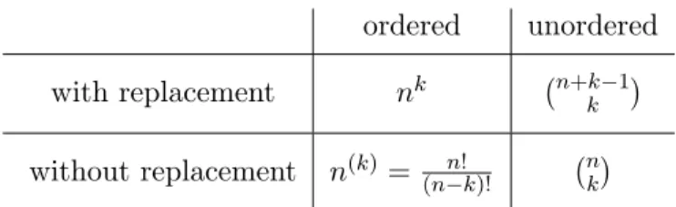
Many combinatorial problems can be viewed as drawing balls. Consider the problem of determining the number of ways of drawing kballs one after the other out of nballs, numbered from 1 to n. The most important cases are summarized in Figure 1.
To give an example that the expressions are true: for the special case in which we draw nballs out ofnballs in an ordered way without replacement, we get the number of all possible ways of permuting nnumbers, which as we know is n!.
ordered unordered with replacement nk ¡n+k−1k ¢ without replacement n(k)= (n−k)!n! ¡nk¢
Figure 1: Number of outcomes of drawing kout of nballs
5.3 Basic concepts in probability theory
Next we introduce some basic concepts in probability theory.
Let us consider a random experiment of which all possible results are included in a non-empty set Ω, usually called the sample space. An element ω ∈ Ω is called a sample point oroutcome of the experiment. An event of a random experiment is specified as a subset of Ω. Event A is called true if an outcome ω∈Ω has been chosen withω ∈A. OtherwiseA is calledfalse. A systemAof events (or, in general, subsets of Ω) is called an algebraif
• Ω∈ A,
• ifA, B∈ A, thenA∪B∈ Aand A∩B∈ A, and
• ifA∈ A, then ¯A∈ A.
Given an algebraA, a function µ:A →IR+ is called a measureon A if for every pair of disjoint sets A, B∈ Awe have
µ(A∪B) =µ(A) +µ(B).
This definition clearly implies thatµ(∅) = 0 and that for any set of pairwise disjoint eventsA1, . . . , Ak∈ A we have
µ Ã k
[
i=1
Ai
!
= Xn
i=1
µ(Ai). Furthermore, it implies that for any pair of setsA, B∈ Awe have
µ(A∪B) =µ(A) +µ(B)−µ(A∩B). We say that a function p:A →[0,1] is aprobability measure if
• p is a measure onA and
• p(Ω) = 1.
Given a probability measure p, theprobabilityof an event A to be true is defined as Pr[A] =p(A).
We say that a triple (Ω,A, p) is a probability space if A is an algebra over Ω and p is a probability measure on A.
5.4 Events
Starting from a given collection of sets that represent events, we can form new events by means of statements containing the logical connectives “or,” “and,” and “not,” which correspond in the language of set theory to the operations “union,” “intersection,” and “complement.”
IfAandBare events, theirunion, denoted byA∪B, is the event consisting of all outcomes realizing eitherA orB. Theintersectionof Aand B, denoted byA∩B, consists of all outcomes realizing both A andB. The differenceofB and A, denoted byB\A, consists of all outcomes that belong toB but not toA. IfA is a subset of Ω, itscomplement, denoted by ¯A, is the set of outcomes in Ω that do not belong toA. That is, ¯A= Ω\A.
Two events A and B are called disjoint if A∩B is empty. In probability theory, ∅ is called the impossibleevent. The set Ω is naturally called the certain event.
If Ω is a countable sample space (i.e., its elements can be arranged in a sequence so that the rth element is identifiable for any r ∈ IN), we define the size of an event A, denoted by |A|, to be the number of outcomes it contains.
5.5 The Inclusion-Exclusion Principle
LetA1, . . . , Anbe any collection of events. Theinclusion-exclusion principlestated earlier implies that Pr
" n [
i=1
Ai
#
= Xn
k=1
(−1)k+1 X
i1<i2<...<ik
Pr
\k
j=1
Aij
. (1)
For the special case ofn= 2 we obtain
Pr[A1∪A2] = Pr[A1] + Pr[A2]−Pr[A1∩A2].
In cases where it is too difficult to evaluate (1) exactly, Bonferroni’s inequalitiesmay be used to find suitable approximations:
• For every odd m,
Pr
" n [
i=1
Ai
#
≤ Xm
k=1
(−1)k+1 X
i1<i2<...<ik
Pr
\k
j=1
Aij
.
• For every even m,
Pr
" n [
i=1
Ai
#
≥ Xm
k=1
(−1)k+1 X
i1<i2<...<ik
Pr
\k
j=1
Aij
.
Special cases of these inequalities are Boole’s inequalities:
Pr
" n [
i=1
Ai
#
≤ Xn
i=1
Pr[Ai] and
Pr
" n [
i=1
Ai
#
≥ Xn
i=1
Pr[Ai]− X
1≤i<j≤n
Pr[Ai∩Aj]. We will give two examples to illustrate the use of these inequalities.
Example 1: Given a set systemM ={S1, . . . , Sm}over some set of elementsV, consider the problem of coloring each element inV with one out of two colors in such a way that no setSiismonochromatic, i.e. contains only nodes of a single color. We would like to identify a class of sets S for which this is always possible. Such a class is given in the following claim.
Claim 5.1 For every set system M of size m in which every set S ∈M is of size at least logm+ 2, there is a 2-coloring of the elements such that no set inM is monochromatic.
Proof. Consider the random experiment of choosing for each element independently and uniformly at random one of the two possible colors. In this case, the probability that a set of sizekis monochromatic is equal to 2·2−k= 2−k+1. For every i∈ {1, . . . , m}, letAi be the event that setSi is monochromatic.
Then, by the inclusion-exclusion principle, Pr[A1∪. . .∪Am]≤
Xm
i=1
Pr[Ai]≤ Xm
i=1
2−(logm+1)= 1 2 . Hence,
Pr[ ¯A1∩. . .∩A¯n] = 1−Pr[A1∪. . .∪An]≥ 1 2 ,
and therefore there must exist a 2-coloring such that no set is monochromatic. ut Example 2: Consider the situation that we havenballs andnbins, and each ball is placed in a bin chosen independently and uniformly at random.
Claim 5.2 The probability that bin 1 has at least one ball is at least 1/2.
Proof. For anyi∈[n], letAi be the event that balliis placed in bin 1. Then, by Boole’s inequality, Pr[bin 1 has at least one ball] = Pr
[
i∈[n]
Ai
≥ X
1≤i≤n
Pr[Ai]− X
1≤i<j≤n
Pr[Ai∩Aj]
= X
1≤i≤n
1
n − X
1≤i<j≤n
1 n2
= 1− Ãn
2
! 1
n2 ≥1−1 2 = 1
2 .
u t
Observe that the probability bound in Claim 5.2 is not far away from the exact bound:
Pr[bin 1 has at least one ball] = 1− µ
1− 1 n
¶n
n→∞= 1−1 e .
5.6 Conditional probability
Theconditional probabilityof eventB assuming an eventAwith Pr[A]>0 is denoted by Pr[B |A]. It satisfies
Pr[B |A] = Pr[A∩B]
Pr[A]
or equivalently,
Pr[A∩B] = Pr[A]·Pr[B|A]. (2)
Expression 5.6 holds, since the space of outcomes that is left for Pr[B |A] is the set of all outcomes in A, and therefore we have to normalize the probabilities of the outcomes inA in a way that they sum up to 1. This is achieved by dividing Pr[A∩B] by Pr[A].
We can generalize Expression 2 as follows: if A1, . . . , An are events with Pr[A1∩. . .∩An−1]>0, then
Pr[A1∩. . .∩An] = Yn
i=1
Pr[Ai |A1∩. . .∩Ai−1].
Suppose thatAandB are events with Pr[A]>0 and Pr[B]>0. Then, in addition to the equality (2), we have
Pr[A∩B] = Pr[B]·Pr[A|B]. (3)
From (2) and (3) we obtain Bayes’s formula
Pr[A|B] = Pr[A]·Pr[B |A]
Pr[B] .
Two events A andB are called independentif and only if Pr[B |A] = Pr[B].
Note that, due to Bayes’s formula, in this case also Pr[A | B] = Pr[A], that is, the independence property issymmetric. Furthermore, it holds that
Pr[A∩B] = Pr[A]·Pr[B].
If Pr[B|A]6= Pr[B], then A and B are said to be correlated. A and B are called
• negatively correlatedif Pr[B |A]<Pr[B] and
• positively correlatedif Pr[B |A]>Pr[B].
By Bayes’s formula, all of these correlation properties are also symmetric.
As an example, any two disjoint events AandB with positive probabilities cannot be independent, since Pr[B | A] = 0. However, they are always negatively correlated. Furthermore, they have the property that
Pr[A∪B] = Pr[A] + Pr[B].
5.7 Random Variables
Any numerical function X =X(ω) defined on a sample space Ω may be called arandom variable. In this lecture we will only consider integer-valued random variables, i.e., functions of the formX: Ω→ZZ.
A random variable X is called non-negative if X(ω) ≥ 0 for all ω ∈ Ω. For the special case that X maps elements in Ω to {0,1}, X is called a binary or Bernoulli random variable. A binary random variable X is called an indicator of event A (denoted by IA) if X(ω) = 1 if and only ifω ∈ A for all ω∈Ω.
For any random variable X and any number x ∈ ZZ, we define [X =x] = {ω ∈ Ω : X(ω) = x}.
Instead of using set operations to express combinations of events associated with random variables, we will use logical expressions in the following, that is,
• instead of Pr[[X=x]∩[Y =y]] we write Pr[X =x∧Y =y], and
• instead of Pr[[X=x]∪[Y =y]] we write Pr[X =x∨Y =y].
Furthermore, we define
Pr[X ≤k] =X
`≤k
Pr[X=`] and Pr[X≥k] =X
`≥k
Pr[X=`].
The function pX(k) = Pr[X=k] is called theprobability distribution of X, and the function FX(k) = Pr[X ≤k] is called the(cumulative) distribution functionof X.
Two random variables X and Y are called independentif, for allx, y∈ZZ, Pr[X=x|Y =y] = Pr[X=x].
5.8 Expectation
The most important measure used in combination with random variables is the expectation.
Definition 5.3 Let (Ω,A, p) denote an arbitrary probability space and X : Ω → ZZ be an arbitrary function with integer values. Then the expectationof X is defined as
E[X] = X
x∈ZZ
x·Pr[X=x]. (4)
The following fact lists some basic properties of the expectation.
Fact 5.4 Let X andY be arbitrary random variables and c be an arbitrary constant.
• E[X+Y] = E[X] + E[Y].
• E[c·X] =c·E[X].
• If X is a binary random variable, then E[X] = Pr[X= 1].
• If X and Y are independent, then E[X·Y] = E[X]·E[Y].
The expectation enables us to prove some simple tail estimates.
Fact 5.5 Let X be an arbitrary random variable. Then
Pr[X <E[X]]<1 and Pr[X >E[X]]<1.
The next result provides a first, simple probability bound that depends on the deviation from the expected value. It has apparently first been used by Chebychev, but it is commonly called Markov inequality.
Theorem 5.6 (Markov Inequality) Let Xbe an arbitrary non-negative random variable. Then, for anyk >0,
Pr[X≥k]≤ E[X]
k . Proof. Obviously,
E[X] =X
x≥0
x·Pr[X =x]≥k·Pr[X≥k].
u t
Next we present a simple example to illustrate the use of these inequalities.
Example: In the first theorem we show that every graph has a bipartite subgraph with at least half of its edges.
Theorem 5.7 Let G = (V, E) be a graph with n vertices and m edges. Then G contains a bipartite subgraph with at least m/2 edges.
Proof. LetT ⊆V be a random subset given by a random experiment with independent probabilities Pr[v ∈T] = 1/2 for every v ∈V. We call an edge{v, w} crossingif exactly one of v, ware in T. Let X be the number of crossing edges. We define
X= X
{v,w}∈E
Xv,w
whereXv,w is the indicator random variable for{v, w} being crossing. Then E[Xv,w] = 1/2
as two fair coin flips have probability 1/2 of being different. Then E[X] = X
{v,w}∈E
E[Xv,w] = m 2 .
Thus, according to Fact 5.5, there must be some choice ofT withX≥m/2 and the set of those crossing
edges forms a bipartite graph. ut
The theorem does not automatically provide an efficient algorithm for finding such a subgraph.
However, the next theorem shows that for a slightly smaller value than m/2 this can easily be done.
Theorem 5.8 There is a randomized algorithm that only needs an expected linear amount of time steps to find a bipartite subgraph in a graph G= (V, E), |E|=m, with at least m/4 edges.
Proof. Let the random variableY be defined asY =m−X, i.e.Y counts the number of non-crossing edges. We would like to have Y as small as possible. From the previous proof and the linearity of expectation we know that
E[Y] =m−E[X] =m−m/2 =m/2.
Hence, it follows from the Markov inequality that Pr[Y ≥3m/4]≤ E[Y]
3m/4 = m/2 3m/4 = 2
3 . Thus, Pr[Y <3m/4]≥1/3 and therefore Pr[X > m/4]≥1/3.
Now, consider the following algorithm:
repeat
perform the random experiment in Theorem 5.7 until at least m/4 edges are crossing
Let the random variableT denote the number of rounds the algorithm needs to produce a bipartite graph with at least m/4 edges. Since each round has a probability of success of some p ≥ 1/3, we obtain that
Pr[T =t] = (1−p)t−1·p . Hence,
E[T] = X
t∈IN
t·Pr[T =t]
= X
t∈IN0
(t+ 1)·(1−p)tp
= p
X
t∈IN0
(1−p)t
2
=p·
µ 1
1−(1−p)
¶2
= 1 p .
Since p≥1/3, it follows that E[T]≤3. ut
5.9 Variance
Definition 5.9 The variance(or dispersion) of a random variableX, denoted by V[X], is defined as V[X] = E[(X−E[X])2].
The number σ=pV[X] is called the standard deviation of X.
The following fact lists some basic properties of the variance.
Fact 5.10 Let X and Y be arbitrary random variables and a, bbe arbitrary constants.
• V[a+b·X] =b2·V[X].
• If X is a binary random variable, then V[X] = E[X]·(1−E[X]).
• If X and Y are independent, then V[X+Y] = V[X] + V[Y].
• If X and Y are independent, then V[X·Y]
E[X·Y]2 =−1 + µ
1 + V[X]
E[X]2
¶ µ
1 + V[Y] E[Y]2
¶ .
The most well-known tail estimate that uses the variance of a random variable is due to Chebychev.
Theorem 5.11 (Chebychev Inequality) Let X be an arbitrary random variable. Then, for every k >0,
Pr[|X−E[X]| ≥k]≤ V[X]
k2 .
Proof. From the Markov inequality it follows for all random variablesX that Pr[|X| ≥k] = Pr[X2 ≥k2]≤E[X2]/k2 .
Replacing |X|by |X−E[X]|yields the theorem. ut
5.10 Higher Order Moments
Expectations of powers of random variables are called moments and play an essential role in the investigations of probability theory. For us they will be of particular interest in the study of sums of random variables. Given a random variable X, the following expected values of functions of X are often studied:
• E[Xk],k∈IN : kth moment ofX
• E[|X|k],k∈IN : kth absolute moment ofX
• E[|X−E[X]|k],k∈IN : kth absolute central moment ofX
• E[eh·X], h >0 : exponential moment ofX
Lo´eve stated the following result in [Lo´e77], which easily follows from the Markov inequality.
Theorem 5.12 (General Markov Inequality) LetXbe an arbitrary non-negative random variable and g be an arbitrary function that is non-negative and non-decreasing on IN0. Then, for any k ≥ 0 with g(k)>0,
Pr[X ≥k]≤ E[g(X)]
g(k) .
Proof. Sinceg is non-negative and non-decreasing on IN0, it holds for every k≥0 that E[g(X)] = X
x≥0
g(x)·Pr[X =x]≥g(k) Pr[X≥k].
u t
5.11 Basic Probability Distributions
In this section we introduce the most important probability distributions used in combination with discrete random variables.
5.11.1 Uniform distribution
A random variableX is calleduniformly distributed over a finite setM of values inIRif Pr[X =x] = 1
|M|
for all x∈M. IfM ={a, a+ 1, . . . , b}for some integers a, bwith a < b, then E[X] = a+b
2 and V[X] = (b−a)2
12 +b−a 6
5.11.2 Binomial distribution
A random variableX is called binomially distributedif there are parameters p∈[0,1] and n∈INsuch that
Pr[X=k] = Ãn
k
!
pk(1−p)n−k for all k∈ {0, . . . , n}. In this case,
E[X] =n·p and V[X] =n·p(1−p).
As an example, consider the situation that we havem balls in an urn, of whichm1 are red and m2 are blue. We draw n balls at random out of this urn, one after the other, replacing each drawn ball.
Let the random variable X denote the number of red balls drawn. Then X is binomially distributed withp=m1/m.
5.11.3 Poisson distribution
A random variableX is calledPoisson distributedif there is a parameter λ >0 such that Pr[X=k] = λk
k! ·e−λ for all k∈IN0. In this case,
E[X] =λ and V[X] =λ .
The binomial distribution converges towards the Poisson distribution if, in the example above, the number of balls in the urn,m, and the number of draws, n, is increased while keeping the number of red balls constant.
5.11.4 Geometric distribution
A random variableX is calledgeometrically distributed if there is a parameterp∈[0,1] such that Pr[X=k] = (1−p)k−1p
for all k∈IN. In this case,
E[X] = 1
p and V[X] = 1−p p2 .
As an example, suppose that we again have an urn with mballs, of which m1 balls are red and m2 balls are blue. We draw a ball at random from this urn and replace it until we draw a red ball. Let the random variable X denote the number of balls drawn. Then X is geometrically distributed with p=m1/m.
5.11.5 Hypergeometric distribution
A random variableX is calledhypergeometrically distributedif there are parametersN,M, andnsuch that
Pr[X=k] =
¡M
k
¢¡N−M
n−k
¢
¡N
n
¢
for all k∈ {0, . . . , n}. In this case, we obtain forp=M/N E[X] =n·p and V[X] = N −n
N −1 ·n·p(1−p).
As an example, consider the situation that we haveN balls in an urn, of whichM are red andN−M are blue. We drawnballs at random out of this urn, one after the other,withoutreplacing each drawn ball. Let the random variableX denote the number of red balls drawn. ThenX is hypergeometrically distributed.
5.12 Chernoff bounds
In the following we study sums of independent binary random variables. Tail estimates for these sums have among many others been investigated by Chernoff [Che52] and are often called Chernoff bounds.
It has been found convenient to use exponential moments of random variables to derive these tail estimates. The idea of using exponential moments was apparently first used by S. N. Bernstein. His method had a significant influence on deriving tail estimates also for many other problems. We present here a proof given by Hagerup and R¨ub [HR90]. Bound (6) was taken from [McD98].
Theorem 5.13 (Chernoff Bound) LetX1, . . . , Xnbe independent binary random variables, letX= Pn
i=1Xi, and let µ= E[X]. Then it holds for all δ≥0 that Pr[X ≥(1 +δ)µ] ≤
à eδ (1 +δ)1+δ
!µ
(5)
≤ e− δ
2µ
2(1+δ/3) (6)
≤ e−min[δ2, δ]·µ/3 . Furthermore, it holds for all 0≤δ ≤1 that
Pr[X ≤(1−δ)µ] ≤
à e−δ (1−δ)1−δ
!µ
(7)
≤ e−δ2µ/2 .
Proof. We will only show (5). For all i ∈ [n], let pi = E[Xi]. According to the general Markov inequality (see Theorem 5.12) we obtain that, for any functiong(x) =eh·x withh >0 and anyδ≥0,
Pr[X≥(1 +δ)µ]≤e−h(1+δ)µ·E[eh·X]. (8) Since X1, . . . , Xn are independent, it follows that
E[eh·X] = E[eh(X1+...+Xn)] = E[eh·X1· · ·eh·Xn] =Qni=1E[eh·Xi]
= Yn
i=1
(pieh+ (1−pi)) =Qni=1(1 +pi(eh−1))
≤ Yn
i=1
epi(eh−1) since 1 +x≤ex for all x
= eµ(eh−1).
This yields together with inequality (8) that
Pr[X≥(1 +δ)µ]≤e−h(1+δ)µ·eµ(eh−1)= e−(1+h(1+δ)−eh)µ. (9) The right-hand side of (9) attains its minimum at h=h0, where h0 = ln(1 +δ). Inserting this in (9) yields
Pr[X≥(1 +δ)µ]≤(1 +δ)−(1+δ)µ·eδ·µ=
à eδ (1 +δ)1+δ
!µ .
This completes the proof for inequality (5). The proof of (7) can be done in a similar way. ut
References
[Che52] H. Chernoff. A measure of asymptotic efficiency for tests of a hypothesis based on the sum of observa- tions. Annals of Mathematical Statistics, 23:493–509, 1952.
[HR90] T. Hagerup and C. R¨ub. A guided tour of Chernoff bounds.Information Processing Letters, 33:305–308, 1989/90.
[Lo´e77] M. Lo´eve. Probability theory. Springer Verlag, New York, 1977.
[McD98] McDiarmid. Concentration. In M. Habib, C. McDiarmid, J. Ramirez-Alfonsin, and B. Reed, editors, Probabilistic Methods for Algorithmic Discrete Mathematics, pages 195–247. Springer Verlag, Berlin, 1998.