Brownian motion

Chapter 7

Brownian motion

The well-known Brownian motion is a particular Gaussian stochastic process with covariance E(w τ w σ ) ∼ min(τ, σ). There are many other known examples of Gaussian stochastic pro- cesses, for example the Ornstein-Uhlenbeck Process or the oscillator process. They all belong to a larger class of processes which are in general not even Gaussian and which we shall discuss in the appendix.

The Brownian process describes the disordered motion of small particles suspended in a liquid. It is believed that Brown studied pollen particles floating in water under the microscope.

He observed minute particles executing a jittery motion. The theory of this motion has been invented by E INSTEIN and S MOLUDCHOWSKI . The mathematically rigorous construction of the corresponding stochastic process has been developed by W IENER .

We have seen that contrary to the complex transition amplitude K (t, q, 0) in ordinary quan- tum mechanics, its continuation K(τ, q, 0) defines a probability density. For the free particle starting at the origin the probability to end up at q after a ’time’ τ is

P 0 (τ, q) =

m 2πτ

d/2

e ^−mq

^/2τ , (7.1)

and the probability to end up in the open set O ⊂

ⁿ is P 0 (τ, O ) =

Z

O dq K 0 (τ, q, 0) ≤ 1. (7.2) P 0 belongs to a Brownian motion, named after the botanist R OBERT B ROWN . Although the mathematical model of Brownian motion is among the simplest continuous-time stochastic pro- cesses it has several real-world applications. An example is stock market fluctuations.

7.1 Diffusion

Diffusion is described by Fick’s diffusion laws [25]. They were derived by A DOLF F ICK in

the year 1855. The first law relates the diffusive flux to the concentration field, by postulating

CHAPTER 7. BROWNIAN MOTION 7.1. Diffusion 61

that the flux goes from regions of high concentration to regions of low concentration, with a magnitude and direction that is proportional to the concentration gradient,

J = − D ∇ φ. (7.3)

Here J is the diffusion flux, D the diffusion coefficient with dimension m ² /s and φ is the con- centration of the diffusing substance. D is proportional to the squared velocity of the diffusing particles, which depends on the temperature and viscosity of the fluid and the size of the parti- cles according to the Stokes-Einstein relation

D = k B T

γ , (7.4)

where γ is the drag coefficient, the inverse of the mobility. For spherical particles of radius r in a medium with viscosity η the drag coefficient is γ = 6πηr. In applications the driving force is a out of equilibrium concentration of particles, a spacial distribution of temperature or a non-vanishing gradient of a chemical potential.

Fick’s second law predicts how diffusion causes the concentration field to change with time τ . It follows from his first law and the continuity equation

∂φ

∂τ = −∇ · J (7.5)

which expresses our expectation that the number of particles is conserved. The change of the number of particles in a given region is equal to the number of particles leaving or entering the region through its boundary. Inserting the continuity equation into (7.3) yields the second law of Fick,

∂φ

∂τ = ∇ · (D ∇ φ). (7.6)

For a constant diffusion coefficient D this law simplifies to

∂φ

∂τ = D △ φ (7.7)

and it has the same form as the heat equation. An important example is the equilibrium case for which the concentration does not change in time, so that the left side of (7.7) is identically zero and △ φ = 0. This is Laplace’s equation, the solutions to which are harmonic functions.

If we start at time 0 with one particle at q ^′ the solution of (7.7) in denoted by K ₀ (τ, q). With the initial condition

K 0 (0, q) = δ(q − q ^′ ) (7.8)

the solution of the diffusion equation is

K 0 (τ, q, q ^′ ) = 1

√ 4πDτ e ^−(q−q

⁾

^/4Dτ (7.9)

CHAPTER 7. BROWNIAN MOTION 7.2. Discrete random walk 62

as can be verified by substitution. This has been known since the beginning of the last century and forms the subject of several textbooks on Brownian motion [26]. This particular solution is just the Euclidean propagator (7.1) if we identify D = 1/2m.

7.2 Discrete random walk

The Brownian motion is the scaling limit of a discrete random walk. This means that if one takes the random walk with very small steps one gets an approximation to Brownian motion.

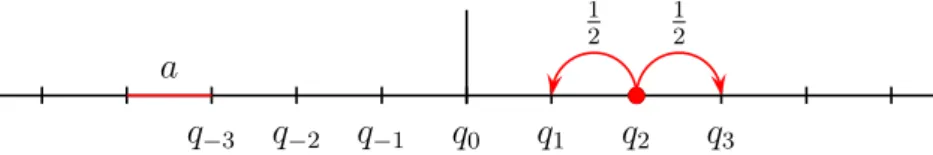
The one-dimensional discrete random walk is the erratic motion of a point particle on a 1- dimensional lattice with lattice spacing a. The particle suffers displacements in form of a series of steps, each step being taken in either direction within a certain period of time, say of length ǫ.

We suppose that forward and backward steps occur with equal probability ¹ ₂ and that successive

q ₀ q ₁ q ₂ q ₃ q −1

q −2

q −3

b

a

1 2

1 2

b

Figure 7.1: The particle may jump with equal probabilities one step to the left or right.

steps are statistically independent. Hence, the probability for a transition from q j = ja to q k = ka during a time ǫ is

P kj = P (ǫ, q k , q j ) =

₁

2 if | k − j | = 1

0 otherwise. . (7.10)

This simple example of a stochastic process (actually a Markov chain) is homogeneous and isotropic,

P (ǫ, q k , q i ) = P (ǫ, q k − q i ) and P (ǫ, q k , q j ) = P (ǫ, q j , q k ). (7.11) After n time-steps the probability to jump from q j to q k is given by the sum of the probabilities of the possible ways of achieving that, which is just

P (nǫ, q _k , q _j ) = ^X

i

,...i

P _ki

P _i

_i

· · · P _i

_i

P _i

_j = (P ⁿ ) _kj . (7.12)

The initial position of the particle may be uncertain and the probability to find it at lattice point

q j is p j . If it sits with certainty 1 at the origin then p j = δ j0 . After n time-steps the system

has evolved and produced a new distribution P ⁿ p. The evolution operators P ⁿ determines the

change of the initial probability distribution after n time-steps.

CHAPTER 7. BROWNIAN MOTION 7.3. Scaling limit 63

It is not difficult to calculate the powers of P . The probability to hop from the lattice site q _j to the site q _k after n time-steps is 1/2 ⁿ times the number of paths on the lattice from q _j to q _k . If n is even then k − j must be even and if n is odd then k − j must be odd. The particle must jump r = ¹ ₂ (n + k − j) steps to the right and ℓ = ¹ ₂ (n + j − k) steps to the left. The number of paths from q j to q k is then equal to the number of ways one can combine r steps to the right with ℓ steps to the left to obtain a path of length n. This number is given by the binomial coefficient.

Hence one finds the following probability P (nǫ, q k − q j ) = 1

2 ⁿ n r

!

= 1 2 ⁿ

n ℓ

!

.

With the help of the identity n r

!

+ n

r − 1

!

= n + 1 r

!

one obtains the difference equation

P (nǫ, q + a) + P (nǫ, q − a) = 2P (nǫ + ǫ, q). (7.13) where q = q _k − q _j denotes the displacement. This equation maybe rewritten as

1

ǫ { P (τ + ǫ, q) − P (τ, q) } = a ² 2ǫ

1

a ² { P (τ, q + a) − 2P (τ, q) + P (τ, q − a) } , (7.14) where τ = nǫ is the time during which the particle jumps.

7.3 Scaling limit

Now we regard the time-interval ǫ and lattice spacing a as being microscopic quantities and perform the scaling limit

a → 0, ǫ → 0 with nǫ = τ, D = a ²

2ǫ fixed. (7.15)

Other scaling limits are possible. For example a → 0 with fixed ǫ would lead to a situation where the particle does not move anymore. The limit a, ǫ → 0 with fixed a/ǫ would lead to a classical theory without fluctuations. But if we keep a ² /ǫ constant then the correlations tend to finite values in this so-called diffusion limit. The constant D is the macroscopic diffusion con- stant. In the macroscopic description q and τ become continuous variables and the difference equation (7.14) converts into a one-dimensional continuous diffusion equation

∂

∂τ P (τ, q) = D ∂ ²

∂q ² P (τ, q). (7.16)

CHAPTER 7. BROWNIAN MOTION 7.3. Scaling limit 64

At the initial time no diffusion has occurred and P (0, q) = δ(q). The solution of the diffusion equation with this initial condition is just the Gaussian function

P 0 (τ, q) = K 0 (τ, q, 0) = 1

√ 4πDτ e ^−q

^/4Dτ . (7.17)

The transition probability for the discrete random walk is replaced by the probability

q

<q lim

<q P (nǫ, q j ) = 1

√ 4πDτ

Z q

q

du e ^−u

^/4Dτ . (7.18) The trivial matrix identity P ⁿ P ^m = P ^n+m turns into the Chapman-Kolmogorov equation

Z

du P ₀ (τ, q − u)P ₀ (σ, u − q ^′ ) = P ₀ (τ + σ, q − q ^′ ). (7.19) Higher dimensions

The extension to higher dimensions is not difficult. For that we note that the lattice-Laplacian in one dimension acts on a function on the lattice as follows,

( △ L f)(q j ) = 1

a ² { f(q j + a) − 2f (q j ) + f (q j − a) } (7.20) such that the probability for a transition (7.10) can be rewritten as

P =

+ a ²

2 △ L . (7.21)

Now we calculate the n’th power of P for n → ∞ and use the scaling laws in (7.15) P ⁿ = 1 + a ²

2 τ /n

ǫ △ L

n

= 1 + Dτ n △ L

_{n n→∞}

−→ e ^{τ D△} , (7.22)

where lim a→0 △ L = △ is the second derivative in the continuum. The kernel h q, τ | e ^{τ D△} | 0 i is just the above distribution P 0 (τ, q). Now the generalization to d dimensions is natural. If j enumerates the lattice points on a d-dimensional hypercubic lattice with lattice spacing a, then the matrix P is given by

P ij =

₁

2d i, j nearest neighbors

0 otherwise or P =

+ a ²

2d △ L , (7.23)

where △ ^L is the lattice Laplacian in d-dimensions, given by

a ² △ L f (q j ) = ^X

k:|k−j|=1

f (q k ) − 2d · f(q j ). (7.24) The factor 1/2d in (7.23) is needed such that the probability to go somewhere is 1. In the scaling limit we end up with a similar result as in one dimension,

n→∞ lim P ⁿ = e ^{τ D△} , nǫ = τ, a ²

2dǫ = D, (7.25)

and the Brownian motion tends to a Gaussian process with Laplacian △ .

CHAPTER 7. BROWNIAN MOTION 7.4. Expectation values and correlations 65

7.4 Expectation values and correlations

In this section we calculate the observable mean values non-observable microscopic quantities.

For example, the probability for a particle starting at the origin to end up in an open set O ⊂

^d after a time τ is found to be

P 0 (τ, O ) =

Z

q∈O K 0 (τ, q, 0) =

1 4πDτ

d/2 Z

O dq e ^−q

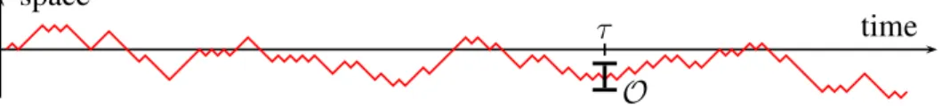
^/4Dτ . (7.26) The event w _τ ∈ O simply means that the Brownian particle has passed the region O at time τ , as sketched in figure 7.2. The probability of finding the particle at time τ 1 in the open set O ¹ , at

τ time

space

O

Figure 7.2: Brownian path starting at q = 0 and passing through the window O at time τ .

time τ 2 > τ 1 in the open set O ² and so on, is P 0 (w τ

∈ O 1 , . . . , w τ

∈ O n ) =

Z

O

dq n · · ·

Z

O

dq 1 P 0 (q n − q n−1 , τ n − τ n−1 )

· · · P ₀ (q ₂ − q ₁ , τ ₂ − τ ₁ )P ₀ (q ₁ , τ ₁ ). (7.27) A stochastic process for which the finite dimensional distributions fulfills these conditions and for which

P 0 (w τ=0 ∈ O ) =

1 if 0 ∈ O

0 otherwise (7.28)

is called a Wiener process. With the distribution P 0 (q, τ ) at hand we can answer all possible questions we may think of.

For example, it is not difficult to check that the expectation value (or mean value) of the position of a Brownian particle is zero,

E(w τ ) =

Z

du u P 0 (τ, u) = 0. (7.29)

The process recalls the starting position 0 since future positions are constrained by (7.29).

E(w τ ) is to be interpreted as a conditional expectation. It is the mean value of w τ , given the information w 0 = 0. Let us calculate the probability that the increment w τ

− w τ

of a Brownian motion starting at the origin assumes some value within the regions O ∈

^d . The answer is

P (w τ

− w τ

∈ O ) =

Z

u

−u

∈O du 2 du 1 P 0 (u 2 − u 1 , τ 2 − τ 1 )P 0 (u 1 , τ 1 )

CHAPTER 7. BROWNIAN MOTION 7.5. Appendix A: Stochastic Processes 66

Changing variables from u ₁ , u ₂ to u ₁ , v = u ₂ − u ₁ we can integrate over u ₁ and obtain

P (w τ

− w τ

∈ O ) = P (w τ

−τ

∈ O ). (7.30) The covariance for the one-dimensional process is

E(w τ w σ ) =

Z

d ² u u 2 P 0 (u 2 − u 1 , τ − σ) u 1 P 0 (u 1 , σ)

= 1

2π √ det Σ

Z

d ² u u 2 u 1 e ^−(u,Σ

^u)/2 ,

where we assumed that τ > σ and used a matrix notation u = u 1

u 2

!

, Σ = 2D σ σ σ τ

!

. The resulting Gaussian integral yields

E(w τ w σ ) = Σ 12 = 2Dσ = 2D min(τ, σ), (7.31) where have already anticipated the result for τ < σ. For the Brownian motion in higher dimen- sions the corresponding result reads

E(w ⁱ _τ w _σ ^j ) = 2Dδ ij min(τ, σ). (7.32) One can show that a typical trajectory w(τ ) of the Brownian motion is continuous. In dimension one it is also recurrent, returning periodically to its origin. Indeed, one can prove the following remarkable theorem:

Theorem: Let B (R, 0) ⊂

^d be the ball with radius R centered at the origin. Then E (w τ ∈ B (R, 0) for one τ ) =

1 for d = 1, 2

< 1 for d ≥ 3.

The times of return of a one-dimensional Brownian motion can serve as a sophisticated random number generator. As a mathematical model it does not only describe the random movement of small particles suspended in a fluid; it can be used to describe a number of phenomena such as fluctuations in the stock market. Trajectories of a Brownian motion are self-similar, a term that is often used to describe fractals. Self-similarity means that for every segment of a given curve, there is either a smaller segment or a larger segment of the same curve that is similar to it.

7.5 Appendix A: Stochastic Processes

In this appendix we collect some useful facts about stochastic processes, since they are related

to the Euclidean path integral. For proofs I refer to the extensive literature on measure theory,

probability and stochastic processes [15]. First we need the definition of a probability space

consisting of a triplet (Ω, A , P ).

CHAPTER 7. BROWNIAN MOTION 7.5. Appendix A: Stochastic Processes 67

• The set Ω is a sample space. An element ω ∈ Ω is called a simple event.

• The second entry A of the triplet denotes a σ-algebra of subsets of Ω called events. A σ-field is closed under complementation, countable intersections and unions,

A, B, A i ∈ A = ⇒ A \ B ∈ A ,

∞

[

i=1

A i ∈ A , Ω ∈ A . (A.1)

• The third entry P is a probability measure. To any event A ∈ A it assigns its probability P (A) ∈ [0, 1]. The probability of the empty set ∅ is zero and that of the sample space Ω is one. The measure has the following natural property

P ( ∪ A i ) = ^X P (A i ) for A i ∈ A , A i ∩ A j = ∅ , i 6 = j. (A.2) A function X : A −→

^d is called Borel-measurable, if the preimage of any Borel set in

^d lies in A ,

X ⁻¹ ( B ) = { ω ∈ Ω | X(ω) ∈ B} ∈ A (A.3) We recall that the Borel sets is the largest σ-algebra containing the open sets in

^d . Let X be Borel-measurable on (Ω, A ). Then X is called P -integrable, if

n→∞ lim

∞

X

k=0

k n P

(

w : k

n < X (w) ≤ k + 1 n

)

≡ J + n→∞ lim

0

X

k=−∞

k n P

(

w : k − 1

n < X(w) ≤ k n

)

≡ J −

both exist. Then one writes

Z

Ω XdP = J + − J − =

Z

X(ω) dP (ω). (A.4)

An A ^′ -measurable map X : A → A ^′ is called random variable. If X is a random variable, then every measure P on A it defines a measure P X on the image A ^′ as follows,

P X (A ^′ ) = P X ⁻¹ (A ^′ ) . (A.5)

P _X is the distribution of X with respect to P . One has the following

Theorem: For every A ^′ -measurable and P X integrable (numerical) function f ^′ on Ω ^′ the func- tion f ^′ ◦ X is P -integrable,

Z

Ω

f ^′ dP _X =

Z

Ω (f ^′ ◦ X) dP. (A.6)

CHAPTER 7. BROWNIAN MOTION 7.5. Appendix A: Stochastic Processes 68

Of particular importance are real-valued random variables P _X . They define measures on Borel sets in

. From the theorem one immediately concludes the

Lemma: If f is Borel measurable on

and X : Ω →

a real random variable, then E(f ◦ X) =

Z

Ω (f ◦ X) dP =

Z

R

f dP X (A.7)

In particular, the expectation value of a random variable is E (X) =

Z

w dP _X (w), (A.8)

and its positive variance is given by

V (X) = E [X − E(X)] ² = E(X ² ) − E ² (X). (A.9) Let X i , i = 1, . . . , n be

-valued random variables and

X ₁ ⊗ . . . ⊗ X _n : Ω −→

ⁿ , ω −→ (X ₁ (ω), . . . , X _n (ω)). (A.10) The corresponding induced measure for the joint distribution is defined by

P X

⊗...⊗X

( B 1 × . . . × B n ) = P X ₁ ⁻¹ ( B 1 ) ∩ . . . ∩ X _n ⁻¹ ( B n ) . (A.11) This should be contrasted with

(P X

⊗ . . . ⊗ P X

) ( B ¹ × . . . × B ⁿ ) = P X ₁ ⁻¹ ( B ¹ ) · · · P X _n ⁻¹ ( B ⁿ ) . (A.12) A number of random variables X ₁ , . . . X _n is called independent if

P X

⊗...⊗X

= P X

⊗ . . . P X

= ⇒ E(X 1 · · · X n ) = E(X 1 ) · · · E(X n ) (A.13) holds true. Important and often used random variables are the Gaussian ones. A random variable is called Gaussian with variance Σ ≥ 0 and mean 0 if

dP X (w) = 1

√ 2πΣ e ^−w

^/2Σ = ⇒ E(X) = 0 and E(X ² ) = Σ. (A.14) For a vanishing variance Σ this simplifies to δ(w)dw. A set of Gaussain random variables X i is joint Gaussian with means E(X i ) = 0 and covariance E(X i X j ) = Σ ij if

P X

⊗...⊗X

(w) = 1

q (2π) ⁿ det Σ e ^−(w,Σ

^w)/2 . (A.15)

After this preparations we introduce the notion of stochastic processes. A stochastic process is

a family of random variables labelled by a (continuous) real parameter. In most application this

parameter is time. More accurately:

CHAPTER 7. BROWNIAN MOTION 7.5. Appendix A: Stochastic Processes 69

Definition: A stochastic process is characterized by a quadruple (Ω, A , P, (X _τ ) _τ∈I ), where (Ω, A , P ) is a probability space and X _τ a family of random variables with values in a common space (E, B ) of states. The parameter space I is typically the half line (0, ∞ ). For every simple event ω ∈ Ω the map τ −→ X τ (ω) is a path of the process.

For a Gaussian stochastic process the X τ

have a joint Gaussian distribution for every finite sequence { τ 1 , . . . , τ n } . Let us relate this rather formal construction to the previously considered Brownian motion. If we identify w(τ) in (7.17) with X τ , then

P (τ, w) ∼ P X

in the present notation. The probability for finding the Brownian particle at time τ in the interval between a and b is

P ( { ω : a ≤ X τ (ω) ≤ b } ) =

Z b

a dP X

(w). (A.16)

Similarly, the probability for finding the particle at times τ i between a i and b i , where 1 ≤ i ≤ n, is given by

P ( { ω : a i ≤ X τ

(ω) ≤ b i } ) =

Z b

a

. . .

Z b

a

dP X

⊗...⊗X

(w 1 , . . . , w n ). (A.17) Here one is naturally led to sets of the form

{ ω | (X τ

⊗ . . . ⊗ X τ

(ω) ∈ B } , B ∈ B ⁿ .

If τ ₁ , . . . , τ _n and n are arbitrary one obtains the set of cylinder sets. They do not form a σ- algebra. In the theory of stochastic processes one uses the σ-algebra generated by this set.

Let us now indicate how one constructs a unique probability measure on the set of paths, that is how one performs the limit from joint distributions on a finite set of random variables to a induced probability measure dP X

. The construction proceeds as follows:

Let J be a subset of the parameter set I and define E ^J = ^Y

τ∈J

E τ , E τ = E and let B ^J = ⊗ ^τ∈J B ^τ (A.18) be the smallest σ-algebra in E J such that the projections

p ^J : E ^J −→ E (A.19)

are measurable. For a finite set J the elements of E ^J may be identified with the corners of a broken line path and for a continuous J as a path J → E. The B ^J is then a σ-algebra on these sets. In addition, let K be a subset of J. Then the projections

p ^J _K : E ^J −→ E ^K , where K ⊂ J ⊂ I (A.20)

CHAPTER 7. BROWNIAN MOTION 7.5. Appendix A: Stochastic Processes 70

are B ^J − B ^K measurable. Next we consider the (E ^J , B ^J ) joint random variable X J = ⊗ ^τ∈J X τ : Ω −→ E ^J , Ω ∋ ω −→ path X τ (ω), τ ∈ J

and let P X

denote the joint distribution of random variables X τ∈J . For example, for the set J = (τ 1 , . . . , τ n ) this means

P X

(B 1 × . . . × B n ) = P { ω | X τ

(ω) ∈ B 1 , . . . , X τ

(ω) ∈ B n } . Since X _K = p ^J _K ◦ X _J we have

P X

= p ^J _K (P X

). (A.21)

Now we need the following definition:

Definition: If the family of probability measures (P X

) with finite J ⊂ I fulfills the condition P X

= p ^J _K (P X

)

for two arbitrary finite subsets K and J with K ⊂ J , then the family is called projective. Now one can prove the following important theorem

Theorem (Kolmogorov): Is E =

ⁿ and B the σ-algebra of it Borel sets and if I is a non-empty set, then to each projective family P _X

of probability measures with finite J on (E ^J , B ^J ) there exists exactly one probability measure P X

on (E ^I , B ^I ) with

p J (P X

) = P X

for all finite J.

One calls P X

the projective limit of the family P X

. The following theorems are useful:

Theorem: Let Σ(τ, σ) be a continuous and real-valued function on I × I, where I is a separable topological space. If for all { τ 1 , . . . , τ n } the function Σ(τ i , τ j ) is positive semi-definite, then there exists a Gaussian process (Ω, A , P, X τ ) with covariance Σ, that is

E (X _τ · X _σ ) = Σ(τ, σ).

To explain the following theorem, due to B OCHNER , we introduce the characteristic function of a random variable,

Definition: Let X be a

^d -valued random variable. Then the Fourier transform of its measure, φ X (j) =

Z

e ^i(j,w) dP X (w) = E e ^i(j,X) (A.22)

is called the characteristic function. The measure P X is uniquely determined by the character-

istic function φ _X of the random variable. Now we can state the

CHAPTER 7. BROWNIAN MOTION 7.5. Appendix A: Stochastic Processes 71

Theorem (Bochner): A function a(j ) is the characteristic function of a random variable if and only if a(j) is continuous, a(0) = 1 and

X z ¯ i a(j i − j j )z j ≥ 0 ∀ j 1 , . . . , j n ∈

; z 1 , . . . , z n ∈

.

The following theorem states, that under certain conditions the measure lives on the set of continuous paths:

Theorem (Kolmogorov-Prehorov): Let (Ω, A , P, X j⊂I ) be a stochastic process. Then one may change the random variables on a set of measure zero such that the new process (Ω, A , P, X ˜ τ⊂I ) is continuous, provided that there exist real numbers a > 0, b > 1, c > 0 such that

E ( | X τ − X σ | ^a ) ≤ c | τ − σ | ^b , ∀ τ, σ ∈

+ .

One concludes that almost all (in the sense of measure theory) Brownian paths are continuous.

One can also prove that almost all Brownian paths are nowhere differentiable.