ESG controversies and controversial ESG: about silent saints and small sinners

Vol.:(0123456789)

https://doi.org/10.1057/s41260-020-00178-x

ORIGINAL ARTICLE

ESG controversies and controversial ESG: about silent saints and small sinners

Gregor Dorfleitner

 · Christian Kreuzer

 · Christian Sparrer

Revised: 15 July 2020 / Published online: 3 August 2020

© The Author(s) 2020

Abstract

Based on an extensive international dataset containing Thomson Reuters environmental, social and corporate governance (ESG) rating, as well as Thomson Reuters newest controversies and combined score of an average of 2500 companies in the years 2002–2018, this article contributes to the existing discourse of the relationship between corporate social perfor- mance and corporate financial performance (CFP) by examining the Fama and French (J Financ Econ 116(1):1–22, 2015) five-factor risk-adjusted performance of positive screened best and worst portfolios, based on a 10 % cutoff, respectively, for equally, value- and rank-weighted strategies in the European, US and global market. Furthermore, the controversies score allows us to examine the mid-to-long-term effects of scandals on the CFP without having to rely on the event study meth- odology. Even though a value-weighted strategy does not show any significant abnormal returns, we examined a significant outperformance for equally weighted worst ESG portfolios and best controversies strategies. These results strongly indicate that this is, on the one hand, driven by low-rated smaller companies (“small sinners”) and clean-coated firms with regard to controversies (“silent saints”) on the other hand. The findings hold for several robustness checks such as adjusting the cutoff rates or splitting the dataset across time.

Keywords ESG · Corporate social responsibility · Corporate social performance · Controversy

Introduction

The interaction between corporate social performance (CSP) measured by ESG scores (which evaluate the performance of companies in their environmental, social or corporate gov- ernance pillars) and their corporate financial performance (CFP) has been the subject of academic research for many years with various findings. This paper is the first to examine the mid-to-long-term effects of controversies, as the new dimension of ESG, on the CFP of listed companies in a portfolio context. Furthermore, it determines the impact of different weighting strategies for high- and low-rated ESG and controversy portfolios.

Since the 1970, the matter of the relationship between CSP and CFP has been investigated by a pile of academic research. Revelli and Viviani (2015) report in their recent meta-analysis that the consideration of CSP in a portfolio

leads to neither an under- nor an outperformance when compared with non-ESG-based investment strategies.

Friede et al. (2015) conclude from their meta-analysis that approximately 90 % of the more than 2000 considered stud- ies report a nonnegative relationship between CSP and CFP.

This heterogeneity of the results can generally be ascribed to three issues, namely the question of how to measure CSP, the methods of stock selection and the question of how to define and measure CFP.

Addressing the first concern, some companies like Sus- tainalytics, MSCI-KLD or Asset4 specialize in issuing an ESG-based rating system and represent therefore as external and independent rating providers a transparent and reliable source of objective corporate social responsibility (CSR) measurements. Nevertheless, Capelle-Blancard and Monjon (2012) as well as Revelli and Viviani (2015) argue that the academic discordance can mainly be ascribed to the factor of data-driven results. Furthermore, Dorfleitner et al. (2015) and Chatterji et al. (2016) report a lack of homogeneous ESG measurement concepts, even among the large interna- tional ESG rating institutions.

*

Gregor Dorfleitner gregor.dorfleitner@ur.de

1

Universität Regensburg, Regensburg, Germany

To address the CSP measurement issue, our analysis includes three distinct ratings that represent industry-based percentile-ranked scores, which enable a simple imple- mentation of a best-in-class approach and therefore do not discriminate any industry groups. The first one, the Thom- son Reuters ESG score (in the following referred to as TR score), evaluates the CSR in various pillars, the Thomson Reuters Controversies score (in the following referred to as controversies score) measures the amount of ESG-based controversies a company encounters during a fiscal year, and finally, the Thomson Reuters combined score (in the follow- ing referred to as combined score) aggregates ESG-related controversies and the TR score of a company.

Despite the fact that the controversies score finds its application within other financial research [see, for exam- ple, Park (2018) and Vasilescu and Wisniewski (2019)], we still contribute to the literature as we are the first ones to consider the extreme event of an ESG-based scandal within the context of portfolio selection.

The heterogeneity of academic results is strengthened even further by the use of various stock selection criteria.

The most common and easy way in which an investor can implement a socially responsible investment (SRI) strategy is represented by socially responsible (SR) mutual funds.

These funds claim to construct a portfolio based on SR selec- tion criteria, such as selecting stocks with a high ESG rating (positive screening) or excluding the so-called sin stocks (tobacco, alcohol, arms or gambling industry) from their investment decisions (negative screening). The majority of the literature devoted to these type of investment strategies reports on no financial performance differences between SR and conventional mutual funds (see, i.e., Statman 2000;

Bauer et al. 2005; Bello 2005; Kreander et al. 2005; Cortez et al. 2009; Utz and Wimmer 2014). However, socially or ethically motivated value-driven investors in particular have to pay close attention to the shifting level of social respon- sibility of these SR funds. Wimmer (2013) finds that these funds are optimized towards their financial rather than their social performance and therefore the overall level of social performance of an SR fund is only persistent in the short run. Utz and Wimmer (2014) argue that, viewed from an individual stock level, neither SR mutual funds nor conven- tional funds differ greatly in terms of portfolio composition.

This leads to the conclusion that SR mutual funds do not sustainably satisfy the needs of value-driven investors.

To overcome the stock selection problem, our analysis does not include SR funds, but rather selects stocks based on an ESG-ranking, allowing us to measure the CSR of a firm directly and therefore constructs long-term ESG-per- sistent portfolios by implementing a monthly rebalanced positive screening process following the ESG-based port- folio formation method of Kempf and Osthoff (2007). We construct a best and worst portfolio based on 10 % cutoffs

for ESG and controversy out- and underperformer in the sample, respectively. Additionally, the best-minus-worst zero-cost-investment strategy simply buys the outperform- ers and short sells the underperformers. Besides testing for the standard approach of value-weighted portfolios, we also conduct equally weighted ones to better control for dispari- ties between large and small firms. Furthermore, we imple- ment a ranked weighting, which, given an ESG-based stock selection, allocates a higher weight to the respective stock the more extreme its score becomes.

Regarding the definition and measurement of CFP, researchers tend to use methods of two different directions.

Whereas the first group, which represents an accounting- based view, defines CFP as the shift in earnings per share (EPS), operating profitability [return on equity (ROE), return on assets (ROA) or return on sales (ROS)] or net income, the second employs a stock-market-oriented perspective by applying (risk-adjusted) performance measurements such as abnormal returns, Sharpe Ratio or Tobin’s Q. A common method in the accounting-based direction comprises the implementation of a particular type of regression analysis.

Qiu et al. (2016), for instance, regress the ROS of companies on their respective ESG score. Mervelskemper and Streit (2017) follow the valuation approach of Ohlson (1995) and add an ESG dimension to the model resulting in a regres- sion of the market-to-book value of equity ratio on an ESG score. Van der Laan et al. (2008) implement a firm-fixed- effects regression to measure the influence of different CSP rating dimensions on the ROA and the EPS. In the stock- market-based perspective, factor models represent a com- mon way in which to measure CFP as they have evolved from simple single-index models (like the CAPM) into a more appropriate approach like the Fama and French (2015) five-factor model. Kempf and Osthoff (2007) and Halbritter and Dorfleitner (2015), for example, align themselves in this group by implementing a Carhart (1997) four-factor model to estimate the abnormal returns of ESG portfolios. With a Fama and MacBeth (1973) regression, Halbritter and Dor- fleitner (2015) also incorporate a cross-sectional approach as they regress the excess return of a certain company on its ESG score. Pintekova and Kukacka (2019) analyze the share prices of companies based on the Thomson Reuters combined score using a within-group fixed-effects model.

Aouadi and Marsat (2018) utilize a fixed-effects model

with dummy variables to estimate the relationship between

Tobins’ Q and an ESG score. Other studies, such as Auer

(2016) and Auer and Schuhmacher (2016) who implement a

Sharpe Ratio approach, rely on financial ratios. Event studies

represent another noteworthy methodology, which is espe-

cially useful when analyzing the short-term impact of certain

events (for example, the eventuation of a scandal). Among

others, Lundgren and Olsson (2009) examine the effects of

environmental-based scandals on firm value by applying a t

test to the cumulative standardized abnormal return, whereas Krüger (2015) utilizes the cumulative abnormal return to show the impact of positive and negative ESG-related news separately on firm value. As these examples show, there is a wide variety of different methods and models for different purposes. A more stock-market-oriented perspective is espe- cially suitable for an analysis from an investor’s perspective as these methods better reflect the investors’ perception of the impact of CSR on the future value of the company (see, i.e., Hillman and Keim 2001; Gentry and Shen 2010; Pinte- kova and Kukacka 2019). Therefore, we align with the stock- market-oriented perspective and use the Fama and French (2015) five-factor model to calculate the risk-adjusted abnor- mal return. Furthermore, the use of the controversy score allows us to directly measure the mid-to-long-term effects of controversies on CFP without having to rely on the event study methodology.

Besides the academic disjointedness, SRI strategies have received a rapid rise in interest over the recent years. The global AUM, according to the Global Sustainable Invest- ment Review GSIA (2018), grew significantly from 22.89$

trillion in 2016 to 30.68$ trillion in 2018, whereas, as reported by the U.S. Forum for Sustainable and Respon- sible Investments USSIF (2018), the AUM experienced a sharp increase from $8.7 trillion in 2016 to $12.0 trillion at the beginning of 2018 in the US market alone, which shows an almost 40 % growth over two years. Furthermore, as mentioned by Crilly et al. (2012), the increasing pressure provided by various stakeholder groups forces companies to invest financial resources in CSR. Moreover, many investors pay close attention to the CSR or CSP of firms, whether they be value-driven investors trying to satisfy their altruistic needs or attempting to achieve abnormal returns by investing in firms with high ESG ratings.

Interestingly, within our results, we find a significant out- performance of up to almost 9 % p.a. for the worst TR score portfolios for equally weighted strategies as well as 7 % p.a.

for the equally weighted best controversies score portfolios.

These results show that investors should focus on low-rated smaller companies (“small sinners”) and clean-coated firms with regard to controversies (“silent saints”). The imple- mentation of a rank-weighted strategy instead of an equally weighted one shows an improvement in alpha across nearly all tested strategies. Regarding the value-weighted strategies, no significant out- or underperformance can be found. These findings apply for different markets and hold true for various robustness checks.

This paper is organized as follows. “Literature overview”

section provides a short overview of the recent state of lit- erature, while the data and methodology are discussed in

“Data and methodology” section. “Results” section presents our results.  “Robustness checks” section implements several robustness checks, and “Conclusion” section concludes.

Literature overview

This section provides an overview of the three perspectives regarding the relationship between CSP and CFP.

The first one indicates a positive relationship between the ESG score of a company and their respective CFP (see, i.e., Kempf and Osthoff 2007; Statman and Glush- kov 2009; Auer 2016; Pintekova and Kukacka 2019) and is often referred to as doing good while doing well. This hypothesis holds true if the costs of socially responsible activities are overestimated or the respective benefits exceed the expectations of the managers and investors.

This can be explained through the managerial myopia the- ory (see, i.e., Narayanan 1985; Stein 1988), where, on the one hand, managers tend to prefer decisions with a short- term profit rather than those that maximize long-term shareholder value, and short-term focused investors, on the other hand, who undervalue long-term benefits. Since the costs of socially responsible activities occur immediately, the benefits of those arise in the future. Therefore, the cor- responding benefits are harder to predict and less attractive to short-term focused investors. Among others, Derwall et al. (2005) and Edmans (2011), who link the doing good while doing well-hypothesis with the managerial myopia theory, conclude that short-term investors are unable (or unwilling) to price the long-term benefits of those activi- ties correctly and therefore undervalue stocks of compa- nies with high levels of engagement in environmental or social aspects, leading to higher returns in the long-run for the respective stocks when compared with other stocks.

This idea of benefit manifestation in the long run is con- sistent with the findings of Dorfleitner et al. (2018), who conclude that the benefits of socially responsible activities (measured by the abnormal stock returns) are produced by unexpected additional cash flows which occur mid-to-long term. Pintekova and Kukacka (2019) divide the term of ESG-based activities into a primary and a secondary sec- tor, whereas the first category refers to socially responsible activities which are closely related to the core business of the respective company. They can corroborate within their results, the point of view of doing good while doing well if the ESG-based activity is located in the primary sector.

The second approach reverts the above-mentioned

relationship, which produces a view of doing good but

not well (see, i.e., Boyle et al. 1997; Barnea and Rubin

2010; Renneboog et  al. 2008; Hong and Kacperczyk

2009). This hypothesis holds true for many reasons. First

of all, based on the idea of Barnea and Rubin (2010),

socially responsible activities that represent lavish expen-

ditures of managers motivated by personal benefits, such

as public appreciation rather than the altruistic motive

of non-financial utility, lead to a significant decrease in

shareholder value and inferior financial performance.

Thus, an agency problem occurs. As described by Krüger (2015), investors will react negatively (positively) to the announcement of socially responsible activities of firms with a high (low) amount of liquidity and can therefore be seen as wasteful investments. Furthermore, as stated by Heinkel et al. (2001) and Hong and Kacperczyk (2009), socially responsible investors and institutions which are subjected to social norm pressures (such as pension funds, universities and religious organizations) exclude

“sin stocks” from their investment decisions resulting in a lower demand, respectively, price and therefore a higher return in comparison with stocks which have a high ESG rating. Another reason supporting the doing good but not well-hypothesis is the trade-off theory stated by Aupperle et al. (1985). In the case of socially responsible invest- ments, the theory argues that ESG-based activities exhaust financial resources which are lacking in other places.

Thus, companies with a low level of expenditure on CSR achieve a competitive advantage in the long run, which may be especially relevant for smaller firms who are on a tighter budget. For small companies, the trade-off theory is strengthened even further by the findings of Aouadi and Marsat (2018). Since they examine the connection between firm visibility, CSP and CFP they conclude that only for high-attention firms (firms that are larger, more present in the media and more greatly observed by analysts), the ESG rating plays a role. In conclusion, if smaller firms invest in CSR, this could be seen as a waste of precious financial resources and therefore reduce firm value.

A third view suggests that there is no clear positive or negative relationship between the CSP and the CFP of a firm. Among others, the recent studies of Halbritter and Dorfleitner (2015) and Auer and Schuhmacher (2016) indi- cate that there is no statistical difference in the risk-adjusted returns of a portfolio consisting of either high ESG-rated or low ESG-rated firms. This third point of view does not nec- essarily conclude the absence of a connection between CSP and CFP but may, in contrast, on the one hand, indicate that the market prices CSP properly which leads to an absence of risk-adjusted returns, or, on the other hand, that the benefits resulting from the ESG-based activities will be offset by their respective drawbacks such as, for example, their costs or the occurrence of agency problems.

Whatever the relationship between CFP and CSP reveals itself to be in a specific context, the question of informational efficient markets still arises. As the stock selection of cor- responding investment strategies is frequently based on the evaluation of certain ESG-based ratings, one may argue, as

these scores are publicly available, that financially motivated investors could not generate a risk-adjusted excess return over conventional or non-ESG-based investments, due to of market efficiency. Fama (1965, (1970) describes, with the efficient market hypothesis (EMH), a framework in which, if the semi- strong form holds true, all information regarding the CSR of a company such as sustainability reports, ESG ratings and even ESG-based scandals should be correctly incorporated into the price of the respective stock shortly after being made public.

Therefore, an outperformance of an ESG-based stock selection strategy would not be possible. However, Grossman (1976) and Grossman and Stiglitz (1980), for example, argue that a perfect information-efficient market could not exist, as there would be no incentive for investors to gather information or to actively manage a portfolio whatsoever, because they could not generate any excess returns.

In the case of SRI, Mynhardt et al. (2017) examine the effi- ciency of socially responsible indices by calculating a Hurst coefficient. The results indicate that most socially responsible indices are significantly less efficient than conventional ones.

With a few exceptions, the Hurst coefficient of most of these

indices differs from an efficient market (where the Hurst coef-

ficient would be exactly 0.5), ranging either from 0.3 to 0.45

(signaling fat tails with an anti-persistent return series which

is negatively correlated) or from 0.55 to 0.6 (indicating fat tails

with a tendency to persistent return series with a slight positive

correlation), which raises the question of whether ESG-based

information is priced immediately and correctly and is con-

sidered in its entirety. This appears to be especially crucial in

terms of ESG-based scandals as, whereas the occurrence of a

scandal is publicly perceived and indeed undoubtedly imme-

diately priced, the impact of the absence of these scandals has

often been overlooked as companies with a low amount of

scandals “fly under the radar”. In this regard, the controversy

score represents a good opportunity to decrease this ineffi-

ciency and can add significant value to ESG investing as this

score is comparable to credit default ratings as these ratings

also evaluate the absence of an infrequent event. Dorfleitner

et al. (2018) also address the aspect of information inefficiency

in the context of SRI as they argue that the future financial

benefits of socially responsible activities are not immediately

perceivable and therefore the economic nature of CSR remains

fairly opaque. Within their results, they conclude that ESG-

based activities lead to significant earnings surprises and unex-

pected additional cashflows in the long run. Edmans (2011)

proves something similar with respect to the intangible asset

of being one of the best companies to work for, due to the

particularly good of their employees.

Data and methodology Data

Due to their transparent scoring methodology, we choose Thomson Reuters

as the world’s largest ESG rating data- base for our data source (see, i.e., Cheng et al. 2014; Durand and Jacqueminet 2015). Therefore, our dataset includes all Thomson Reuters scores (in the following referred to as TR scores), controversies and combined scores for the Euro- pean, US, as well as the global market (including the US and European market) in the period under review from 2002 to 2018. These three scores represent the starting point for further calculations and are explained in more detail below.

First, the controversies scores, which pertain to Thomson Reuter’s latest scoring methodology, add a new dimension to previous approaches by capturing negative media stories from global media sources. This score is a percentile ranking that takes ESG-based scandals into account concerning and infringing on any of the following controversy topics and that occur during a company’s fiscal year. Its rating method- ology consists of 23 ESG controversy topics such as “con- troversies privacy” or “business ethics controversies” (see Thomson Reuters 2019). This score is also benchmarked on the respective industry groups.

Thus, if a scandal occurs, it has a negative impact on the evaluation of the company involved. Ongoing legisla- tion disputes, lawsuits and fines may also affect the ensuing years and may still be visible in further controversy ratings.

Furthermore, the valuation is as follows:

In brief: the fewer scandals that affect a company, the higher its score is.

The TR score evaluates a company’s environmental, social and corporate governance performance (ESG) with regard to ten main categories based on publicly avail- able company-reported data. Each of these categories (for instance, resource use, innovation and emissions in the envi- ronmental pillar, human rights and workforce in the social pillar and management in the corporate governance pillar) receives an individually calculated category score and a related category weighting within its associated pillar. These data result in three so-called pillar scores, one for each ESG pillar. To calculate the overall ESG score, these pillar scores (1)

score

=

# comp. with a worse value+# comp. with the same value included current one 2

# comp. with a value

are aggregated

and in the last step, the TR score is ranked by percentile and benchmarked against the industry. There- fore, the TR score implies an easy way to implement a best- in-class approach (see Thomson Reuters 2019).

Next, the combined score comprises both the TR and the controversies score and thus offers a broadly diversi- fied scoring with regard to performance-based ESG data and controversies collected from worldwide media sources (see Thomson Reuters 2019). The controversies score has no impact on the TR score if it is greater than or equal to 50. In this case, the combined score equals the TR score. However, if the TR score is less than the controversies score, the com- bined score also equals the TR score. Only if the TR score is greater than the controversies score ( < 50 ), the combined score equals the average of both scores.

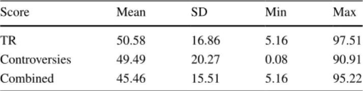
In order to determine our data universe, we only consider companies for which all three ratings are present. Moreover, penny stocks are deleted. As a result, we obtain a monthly- based dataset with over 529,000 observations in total at an average of approximately 2500 companies in a single month during our time period of 2002–2018 (192 months), more precisely between 900 and 4700 at each point in time. For all observed companies, we have a comparable dataset of the three ratings (TR, combined and controversies). Table 1 shows the descriptive statistics of our data universe.

Concerning the TR rating, the mean value of the rating universe corresponds almost exactly to 50 with a standard deviation of approximately 17. The controversies score is approximately the same as the TR score in terms of mean value and standard deviation. As can be expected with regard to the calculation, the combined score has a lower mean value than the TR and controversies score with a standard deviation of 15.

Regarding the correlation between the three scores it is noteworthy that the correlation between the controver- sies score and the TR score is negative (− 0.3107). Thus,

Table 1

Descriptive statistics

This table presents the mean, standard deviation, minimum and maxi- mum values of the TR, controversies and combined scores of the full dataset

Score Mean SD Min Max

TR 50.58 16.86 5.16 97.51

Controversies 49.49 20.27 0.08 90.91

Combined 45.46 15.51 5.16 95.22

1

The scores are currently published by Refinitiv.

2

For more detailed information on the calculation, see Thomson Reuters (2019).

3

The weightings of the three pillars are 34% for the environmental, 35.5% for the social and 30.5% for the governance pillar.

4

For more detailed information on the calculation, see Thomson

Reuters (2019).

companies with a high TR score tend to have a low contro- versies score.

One explanation for this may be that companies that tend to have high ESG scores are affected more greatly by con- troversies, as reflected by the saying “the higher you fly, the harder you fall”.

Furthermore, as would be expected from the composi- tion, the correlation between TR score and combined score is positive (0.7774) as well as between controversies score and combined score (0.3077).

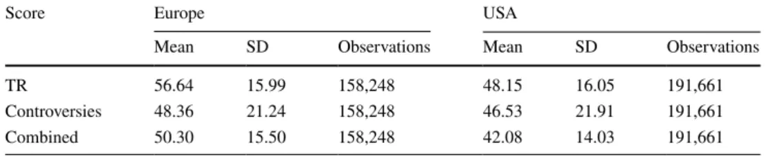
The analysis in this paper is carried out from the per- spective of an US investor, so all data is converted into US dollars. The total returns and market capitalization of the considered companies are received from Thomson Reuters Eikon. Discarded (delisted) or insolvent companies are con- sidered until the last available rating or financial informa- tion. Thus, our results are not influenced by a potential sur- vivorship bias. For more detailed insights, some descriptives for the European and US market are displayed in Table 2.

While for the European market we consider over 158,000 observations based on an average of approximately 820 companies (between 400 and 1000), for the US market, our data consist of over 191,000 observations at an average of approximately 1000 companies (between 400 and 2300).

Methodology

As a first step, we construct several portfolios by generally sorting stocks according to each score. To calculate the monthly returns, we select the best-rated and worst-rated stocks, respectively, and combine them in a portfolio, one being for each of the three scores. Following this procedure, we consider a best-only and worst-only strategy as well as a best-minus-worst strategy, which is long in the best-perform- ing companies and short in the worst-performing ones. As a next step, we consider three different weighting approaches upon which to construct the portfolios. We include the com- mon value-weighted and equally weighted strategies and also a rank-weighted strategy that we present in detail below in “ A different approach: rank-weighted portfolios” section.

We obtain nine stock portfolios

for value- and equally weighted and rank-weighted strategies, which is the object of contemplation in “Rank-weighted portfolios” section,

respectively, in the European, US and global market—in total 27 per market. In order to determine the performance of our portfolios, we apply the Fama and French (2015) five- factor model, which is based on the regression:

In this model, the return of portfolio i for period t is repre- sented by R

while R

comprises the risk-free return. R

denotes the return of the market portfolio, SMB

represents the small-minus-big factor (returns of small stocks minus returns of big stocks) and HML

is the performance differ- ence between companies with a high and low book-to-mar- ket value. The factor RMW

indicates the difference between the returns of stocks with a weak and a robust profitability.

CMA

describes the returns of conservative (i.e., low-invest- ment firms) minus aggressive (i.e., high-investment firms) stocks. Moreover, b

, s

, h

, r

, and c

are the estimated regres- sion coefficients which are calculated by OLS regression, in which e

denotes a (zero-mean) residual and a

the intercept.

Since a Breusch and Pagan (1979) test applied to all port- folios indicates that the residuals of the regressions are sub- ject of heteroskedasticity and a Godfrey (1978) and Breusch (1978) test as well as a Durbin and Watson (1971) test show autocorrelations for most of the models, we use the approach of Newey and West (1987) to calculate standard errors.

A different approach: rank‑weighted portfolios Besides equally weighted and value-weighted portfolios, we also consider a new portfolio composition strategy fol- lowing a similar approach to Frazzini and Pedersen (2014) which reflects the great importance of the ESG ratings for those investors, who may wish to award a different level in the scores through a corresponding weight. Consequently, we build portfolio weights based on the respective score placements. Our new approach is to award better scores and to consequently include them with higher weights in R

− R

= a

+ b

( R

− R

) + s

SMB

+ h

HML

(2)

+ r

RMW

+ c

CMA

+ e

.

Table 2

Descriptive statistics for the European and US market

This table presents the mean, standard deviation and number of observations of the TR, controversies and combined scores of the European and US datasets

Score Europe USA

Mean SD Observations Mean SD Observations

TR 56.64 15.99 158,248 48.15 16.05 191,661

Controversies 48.36 21.24 158,248 46.53 21.91 191,661

Combined 50.30 15.50 158,248 42.08 14.03 191,661

5

This results from three different scores and three different portfolio

sets.

a best-portfolio strategy and vice versa in order to reward worse scores with higher weights in the worst portfolio.

In addition, the best portfolios constructed this way have, by definition, a higher ESG rating than value-weighted or equally weighted strategies, whereas the worst portfolios have lower ratings. First, we determine the best and worst stocks. Next, we divide the companies up by rank in ascend- ing and descending order. In the best portfolios, the company with the highest score receives the (numerically) highest rank. In contrast, the company with the worst score receives the highest rank in the worst portfolios. To calculate the weights w

of a company c ∈ C

⊆ C , where C is the set of all companies within the respective data and C

is the set of all companies within the portfolio at time t, we use

and for each t ∈ T there holds

where Rk

( c ) note the rank of a company c at t, N

= | C

| the cardinality of the portfolio selection at t, in the monthly period under review. If a company c ̂ ∈ C � C

does not appear in the portfolio selection at time t by definition, its weight is

Results

Equally and value‑weighted portfolios

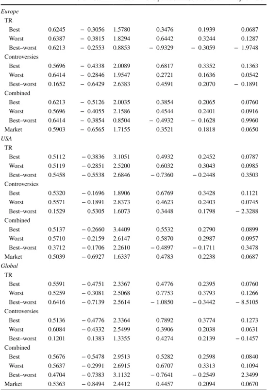
Table  3 presents some measures of all 27 equally weighted 10% portfolio strategies. Concerning the Sharpe ratio, the Sortino ratio and the Treynor ratio, it is noteworthy that all controversies best and TR worst portfolios show higher val- ues than the respective market portfolio, which is a first indi- cation that the performance of these portfolios is high. Fur- thermore, most best and worst portfolios have a higher risk than their respective market in terms of maximum drawdown (MDD), while the controversies best-minus-worst portfolios have a much lower risk in all three markets. Additionally, the MDD is lower than that of the corresponding market for the following portfolios: combined best-minus-worst (US, global), controversies best (Europe, global), TR worst (global) and combined worst (European).

To examine a potential over-performance of the strate- gies in more detail, we consider the alphas of the respec- tive portfolios. The results of the Fama and French (2015) w

∶ C

× T ⟶ [0, 1]

(c, t) ⟼ w

(c, t) = ( N

− Rk

( c )) + 1

∑

̃

c∈C_t

Rk

( c ̃ )

∑

c̃∈C_t

w

( c, t) = ̃ 1,

w

(̂ c, t) ∶= 0.

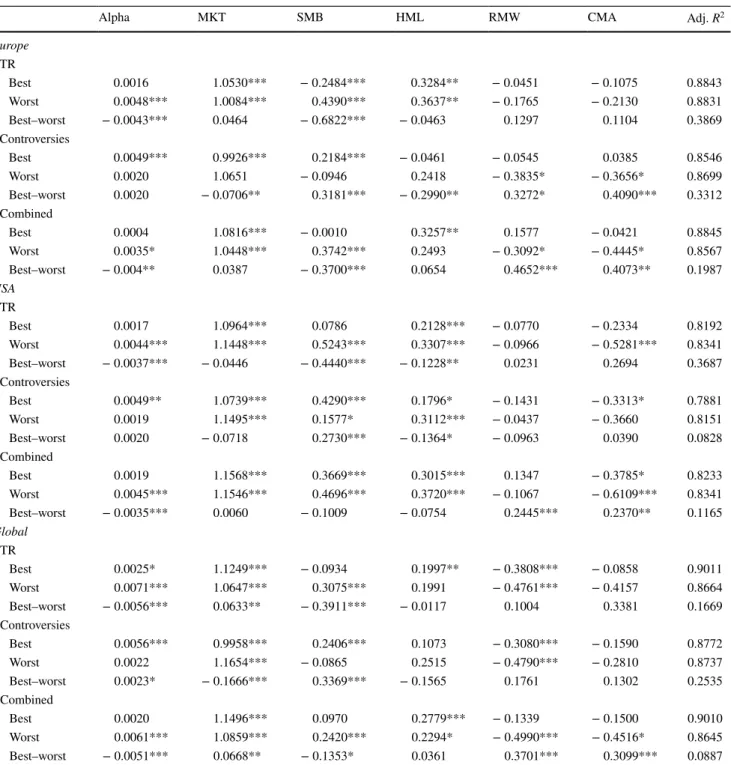
five-factor regressions are presented in Table 4 for equally weighted portfolios and in Table 5 for value-weighted port- folios. Some results immediately catch the eye: Regarding the equally weighted strategy, the worst portfolios based on the TR and combined scores, as well as the best portfolios of the controversies score, indicate positive and significant outperformance. For the controversies score best portfolios, consistently positive and significant alphas can be observed for all portfolios. These portfolios show strongly significant returns of up to almost 7% p.a.

In contrast to this, the con- troversies score worst and best-minus-worst portfolios do not exhibit any striking features.

Surprisingly, when considering combined score portfo- lios, a best portfolio strategy does not lead to a significant performance. However, the performance of the worst port- folio shows a consistently strong and significant outper- formance of up to about 7.6% p.a., which can be observed in all three markets. As a result of this, the calculations indi- cate a significant underperformance of the best-minus-worst portfolios. Therefore, this effect cannot be caused by the controversies score, but instead appears to be determined by the second component of the combined score, namely the TR score.

When taking a closer look at the ESG portfolios, we notice the following. While the performance of the best portfolios—apart from a slight significance in the global market—does not show any over-performance, a strongly significant outperformance of up to almost 9% ( 8.86% ) p.a.

can be observed for the worst TR score portfolios in all three markets. These results resemble those of the combined score portfolios.

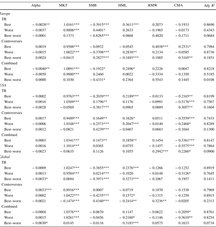
On the contrary, we compare this with the results of the value-weighted portfolios in Table 5. Apart from very few exceptions neither best nor worst portfolios based on the three ratings obtain any ongoing positive and significant alphas within the European, US or global market. So, it becomes relatively clear that there are no ongoing tenden- cies recognizable in terms of any benefits of best or worst strategies. Apart from some isolated outliers, the results lead us to the assumption that the value-weighted strategy does not result in any excess return for investors, which is consist- ent with the findings of Halbritter and Dorfleitner (2015).

It should also be pointed out that the adjusted R

values of all long and short portfolios are consistently high, which indicates a strong explanatory power of our underlying fac- tor model.

There is a clearly recognizable difference between Tables 4 and 5: since the results of the value-weighted and the equally weighted portfolios are very distinct, this

6

The annualized performance of the global controversies score best

portfolio is:

.

points to the fact that the significant outperformance of the equally weighted portfolios is strongly driven by the small companies. In particular, the TR portfolios support the above finding as the equally weighted portfolios based

on low TR scores achieve strong outperformance. These results provide some evidence of the trade-off hypothesis (see Aupperle et al. 1985), as investors appear to reward smaller companies for not investing their money in ESG

Table 3

Measures for equally weighted 10% portfolios

This table shows the maximum drawdown (MDD), skewness, kurtosis (excess), Sharpe ratio, Sortino ratio and Treynor ratio for portfolios from 2002 to 2018. The variables are calculated individually for each equally weighted portfolio based on a 10% cutoff of each score, market and portfolio set as well as for the respective total market

MDD Skewness Kurtosis Sharpe ratio Sortino ratio Treynor ratio Europe

 TR

  Best 0.6245 −  0.3056 1.5780 0.3476 0.1939 0.0687

  Worst 0.6387 −  0.3815 1.8294 0.6442 0.3244 0.1287

  Best–worst 0.6213 −  0.2553 0.8853 −  0.9329 −  0.3059 −  1.9748  Controversies

  Best 0.5696 −  0.4338 2.0089 0.6817 0.3352 0.1363

  Worst 0.6414 −  0.2846 1.9547 0.2721 0.1636 0.0542

  Best–worst 0.1652 −  0.6429 2.6383 0.4591 0.2070 −  0.1891

 Combined

  Best 0.6213 −  0.5126 2.0035 0.3854 0.2065 0.0760

  Worst 0.5696 −  0.4055 2.1586 0.4544 0.2401 0.0916

  Best–worst 0.6414 −  0.3854 0.8504 −  0.4932 −  0.1628 0.9960

 Market 0.5903 −  0.6565 1.7155 0.3521 0.1818 0.0650

USA  TR

  Best 0.5112 − 0.3836 3.1051 0.4932 0.2452 0.0787

  Worst 0.5119 − 0.2851 2.5200 0.6032 0.3043 0.0985

  Best–worst 0.5458 − 0.5538 2.6846 − 0.7360 − 0.2448 0.3503

 Controversies

  Best 0.5320 − 0.1696 1.8906 0.6769 0.3428 0.1121

  Worst 0.5571 − 0.1891 2.8373 0.4623 0.2403 0.0745

  Best–worst 0.1529 0.5305 1.6073 0.3448 0.1798 − 2.3288

 Combined

  Best 0.5137 − 0.2660 3.4409 0.5532 0.2790 0.0899

  Worst 0.5710 − 0.2159 2.6147 0.5870 0.2987 0.0957

  Best–worst 0.3712 − 0.1706 2.2610 − 0.4897 − 0.1711 0.3478

 Market 0.5039 − 0.6927 1.6337 0.4783 0.2238 0.0687

Global  TR

  Best 0.5591 − 0.4751 2.3367 0.4776 0.2395 0.0760

  Worst 0.5259 − 0.3081 2.5068 0.7753 0.3793 0.1266

  Best–worst 0.6416 − 0.7139 2.5614 − 1.0850 − 0.3442 − 8.5105  Controversies

  Best 0.5136 − 0.4776 2.3364 0.7892 0.3774 0.1273

  Worst 0.6084 − 0.4332 2.5499 0.3906 0.2038 0.0631

  Best–worst 0.1201 0.1383 1.3355 0.4274 0.2139 − 0.1457

 Combined

  Best 0.5676 − 0.5478 2.9513 0.5282 0.2598 0.0840

  Worst 0.5637 − 0.2991 2.6915 0.6707 0.3313 0.1094

  Best–worst 0.4704 − 0.7383 3.1132 − 0.7641 − 0.2549 2.3499

 Market 0.5363 − 0.8494 2.4412 0.4457 0.2094 0.0670

improvements. They may consider this spending as a wasteful investment and prefer companies that invest in growth and innovation. As no or even negative significant results were shown for value-weighted best portfolios, we

can conclude that, for large companies, the benefits of expenditures improving CSP are already reflected in the stock price of these companies.

Table 4

Equally weighted 10% portfolios: regressions based on the three observed markets

This table shows the results of the Fama and French (2015) five-factor regression for portfolios from 2002 to 2018 on a monthly basis. The regressions are calculated individually for each equally weighted portfolio based on a 10% cutoff of each score, market and portfolio set. The best (worst) portfolios consist of the 10% best (worst) rated companies regarding a particular score. The best–worst portfolios are long in the best-performing companies and short in the worst-performing ones. Monthly alphas, all estimated coefficients of the five Fama and French (2015) factors and adj. R

are reported upon. In order to estimate standard errors, we use the Newey and West (1987) procedure

***, ** and * indicate a significance level of 1%, 5%, and 10%

Alpha MKT SMB HML RMW CMA Adj. R

Europe  TR

  Best 0.0016 1.0530*** − 0.2484*** 0.3284** − 0.0451 − 0.1075 0.8843

  Worst 0.0048*** 1.0084*** 0.4390*** 0.3637** − 0.1765 − 0.2130 0.8831

  Best–worst − 0.0043*** 0.0464 − 0.6822*** − 0.0463 0.1297 0.1104 0.3869

 Controversies

  Best 0.0049*** 0.9926*** 0.2184*** − 0.0461 − 0.0545 0.0385 0.8546

  Worst 0.0020 1.0651 − 0.0946 0.2418 − 0.3835* − 0.3656* 0.8699

  Best–worst 0.0020 − 0.0706** 0.3181*** − 0.2990** 0.3272* 0.4090*** 0.3312

 Combined

  Best 0.0004 1.0816*** − 0.0010 0.3257** 0.1577 − 0.0421 0.8845

  Worst 0.0035* 1.0448*** 0.3742*** 0.2493 − 0.3092* − 0.4445* 0.8567

  Best–worst − 0.004** 0.0387 − 0.3700*** 0.0654 0.4652*** 0.4073** 0.1987

USA  TR

  Best 0.0017 1.0964*** 0.0786 0.2128*** − 0.0770 − 0.2334 0.8192

  Worst 0.0044*** 1.1448*** 0.5243*** 0.3307*** − 0.0966 − 0.5281*** 0.8341

  Best–worst − 0.0037*** − 0.0446 − 0.4440*** − 0.1228** 0.0231 0.2694 0.3687

 Controversies

  Best 0.0049** 1.0739*** 0.4290*** 0.1796* − 0.1431 − 0.3313* 0.7881

  Worst 0.0019 1.1495*** 0.1577* 0.3112*** − 0.0437 − 0.3660 0.8151

  Best–worst 0.0020 − 0.0718 0.2730*** − 0.1364* − 0.0963 0.0390 0.0828

 Combined

  Best 0.0019 1.1568*** 0.3669*** 0.3015*** 0.1347 − 0.3785* 0.8233

  Worst 0.0045*** 1.1546*** 0.4696*** 0.3720*** − 0.1067 − 0.6109*** 0.8341

  Best–worst − 0.0035*** 0.0060 − 0.1009 − 0.0754 0.2445*** 0.2370** 0.1165

Global  TR

  Best 0.0025* 1.1249*** − 0.0934 0.1997** − 0.3808*** − 0.0858 0.9011

  Worst 0.0071*** 1.0647*** 0.3075*** 0.1991 − 0.4761*** − 0.4157 0.8664

  Best–worst − 0.0056*** 0.0633** − 0.3911*** − 0.0117 0.1004 0.3381 0.1669

 Controversies

  Best 0.0056*** 0.9958*** 0.2406*** 0.1073 − 0.3080*** − 0.1590 0.8772

  Worst 0.0022 1.1654*** − 0.0865 0.2515 − 0.4790*** − 0.2810 0.8737

  Best–worst 0.0023* − 0.1666*** 0.3369*** − 0.1565 0.1761 0.1302 0.2535

 Combined

  Best 0.0020 1.1496*** 0.0970 0.2779*** − 0.1339 − 0.1500 0.9010

  Worst 0.0061*** 1.0859*** 0.2420*** 0.2294* − 0.4990*** − 0.4516* 0.8645

  Best–worst − 0.0051*** 0.0668** − 0.1353* 0.0361 0.3701*** 0.3099*** 0.0887

Looking at the data, it becomes apparent that an equally weighted portfolio strategy based on a high controver- sies score leads to a high outperformance. Therefore, this demonstrates that small companies in particular generate

a sustained stock performance if they have a “clean coat”

with regard to controversies. Thus, one might say that they

“fly under the radar”.

Table 5

Value-weighted 10% portfolios: regressions based on the three observed markets

This table shows the results of the Fama and French (2015) five-factor regression for portfolios from 2002 to 2018 on a monthly basis. The regressions are calculated individually for each value-weighted portfolio based on a 10% cutoff of each score, market and portfolio set. The best (worst) portfolios consist of the 10% best (worst) rated companies regarding a particular score. The best–worst portfolios are long in the best- performing companies and short in the worst-performing ones. Monthly alphas, all estimated coefficients of the five Fama and French (2015) factors and adj. R

are reported upon. In order to estimate standard errors, we use the Newey and West (1987) procedure

***, ** and * indicate a significance level of 1%, 5% and 10%

Alpha MKT SMB HML RMW CMA Adj. R

Europe  TR

  Best − 0.0028** 1.0161*** − 0.3915*** 0.3611*** 0.2073 − 0.1933 0.8690

  Worst − 0.0037 0.8806*** 0.4401* 0.2633 − 0.1965 − 0.0173 0.4343

  Best–worst − 0.0001 0.1373 − 0.8265*** 0.0868 0.4020 − 0.1711 0.0684

 Controversies

  Best 0.0019 0.9588*** − 0.0932 − 0.0545 0.4038*** 0.2531* 0.7984

  Worst − 0.0015 1.0022*** − 0.3708*** 0.2838** 0.2134 − 0.0585 0.8736

  Best–worst 0.0024 − 0.0415 0.2827*** − 0.3493*** 0.1885 0.3165** 0.1851

 Combined

  Best − 0.0040** 1.0891*** − 0.1922* 0.2496* 0.2226 0.0047 0.8218

  Worst − 0.0050 0.9880*** 0.2460 0.0022 − 0.3334 − 0.1350 0.5185

  Best–worst 0.0000 0.1030 − 0.4331* 0.2364 0.5543 0.1445 0.0108

USA  TR

  Best − 0.0002 0.9763*** − 0.2039*** 0.2189*** − 0.0133 − 0.2165** 0.8199

  Worst 0.0016 1.0369*** 0.1796** 0.1176 − 0.0991 − 0.5176*** 0.7567

  Best–worst − 0.0028 − 0.0569 − 0.3817*** 0.0965 0.0889 0.3057** 0.1604

 Controversies

  Best 0.0017 0.9489*** 0.1649** 0.1628* 0.0511 − 0.3559*** 0.7433

  Worst − 0.0006 1.0348*** − 0.2573*** 0.2047*** − 0.0140 − 0.2468* 0.8289

  Best–worst 0.0012 − 0.0821 0.4239*** − 0.0467 0.0683 − 0.1044 0.1300

 Combined

  Best 0.0003 1.0341*** 0.1473** 0.1858** 0.1454 − 0.3361*** 0.8147

  Worst 0.0016 1.1014*** 0.0365 0.0755 − 0.1457 − 0.5575*** 0.7864

  Best–worst − 0.0023 − 0.0635 0.1126 0.1055 0.2942*** 0.2260* 0.0900

Global  TR

  Best − 0.0009 1.0247*** − 0.3855*** 0.2376*** − 0.1266 − 0.1252 0.8919

  Worst 0.0013 0.9584*** 0.0214*** − 0.1020 − 0.0148 − 0.3126* 0.7645

  Best–worst − 0.0033* 0.0694 − 0.3971*** 0.3273*** − 0.1067 0.1957 0.1411

 Controversies

  Best 0.0033*** 0.8916*** 0.0007 − 0.0719 0.1870 − 0.1538 0.7969

  Worst 0.0002 1.0422*** − 0.4235*** 0.1572* − 0.1315 − 0.1250 0.8915

  Best–worst − 0.0021 − 0.1474*** 0.4340*** − 0.2414** 0.3236** − 0.0205 0.2313

 Combined

  Best − 0.0004 1.0376*** − 0.0670 0.1147 − 0.0622 − 0.2059* 0.8761

  Worst 0.0015 1.0261*** − 0.0456 − 0.2160* − 0.1146 − 0.3610** 0.8254

  Best–worst − 0.0030* 0.0145 − 0.0116 0.3183*** 0.0575 0.1633 0.0734

Last but not least, the above observations also find their reflection in the combined score portfolios. On the one hand, the effect of the TR worst portfolios also occurs in the combined score worst portfolios, which are by definition strongly influenced by the TR score. On the other hand, it is not surprising that a slight decrease in the returns appears in these portfolios compared with corresponding TR worst portfolios, which can be explained due to the influence of the controversies score.

To discuss these results against the background of current literature, it is necessary to divide this step into two parts.

As already published by previous studies such as Halbritter and Dorfleitner (2015), we confirm the recent observation, being that a market-weighted ESG strategy does not result in ongoing significant overperformance, so for this strategy, there is no clear out- or underperformance of best or worst portfolios.

The hypothesis of a positive relationship between the CSP and the CFP of a company (see, e.g., Kempf and Osthoff 2007) could only partly be confirmed. Evidently, there is no performance loss when investing in ESG portfolios, but the data suggest that there is also no ongoing positive outper- formance for companies with high ESG ratings, so for these portfolios, we strongly support the results of Revelli and Viviani (2015), being that neither weaknesses nor strengths can be detected for value-weighted positive CSP strategies.

However, this is reverted when considering equally weighted portfolios. Remarkably, no significant negative performance is detected when investing in best ESG port- folios with an equally weighted strategy. Thus, there are no ESG-based performance losses for investors. Moreover, Stat- man and Glushkov (2009) find that investors can achieve positive abnormal returns with socially responsible top- minus-bottom strategies using equally weighted portfolios.

Thus, in relation to the results of our best–worst portfolios, there is no reason for investors to pursue this strategy nowa- days because, in particular, the worst portfolios based on the TR score reveal a significant overperformance. However, this also stands in contradiction to Auer (2016), who claims that investors should eliminate firms with the worst ESG ratings, whereas we find evidence of the fact that these rep- resent some potential for (ESG neutral) investors. Moreover, this finding contradicts even Kempf and Osthoff (2007), who use a long-short strategy and obtain an overperformance.

Contrary to this and related to our results, doing good while doing well did not manifest itself at all during our work.

Market efficientists would expect an immediate reaction on the stock market in the face of a controversy. Therefore, no long-term overperformance can be expected with regard to market-efficiency aspects, so it is surprising that there are several corresponding findings for the controversies score portfolios. Although the occurrences of controversies may be immediately priced by the market, which is indicated by

the non-existing underperformance of the worst controver- sies score portfolio, the absence of controversies appears to be incorrectly evaluated for small companies. The significant outperformance of the best-rated companies therefore indi- cates a less efficient market regarding ESG-based informa- tion as discussed by Edmans (2011), Mynhardt et al. (2017) and Dorfleitner et al. (2018). Smaller companies without an unwanted boost in public perception due to a controversy remain “silent saints” so-to-speak and “fly under the radar”.

The controversies score enables a valuation of controversies that do not take place and may therefore be a good tool to enhance ESG investment as it reveals companies with a low amount of scandals with a specific potential for an increase in market value and stock price.

An additional consideration of the Fama and French fac- tor coefficients yields some interesting insights regarding the differences between value and equally weighting. First, it can be seen that the market betas are generally around 1, but tend to be lower for value-weighted portfolios. This is not surprising, as smaller companies may have higher mar- ket betas and these companies are represented with higher weights in the equally weighted portfolios. Second, we notice that the controversies best, TR worst and combined worst equally weighted portfolios have significant positive SMB

factor coefficients and reveal a higher absolute value compared to the respective value-weighted portfolios, which is again explainable by the higher weights for smaller com- panies. Third, the remaining factors show no systematically deviating patterns.

Portfolios based on market capitalization

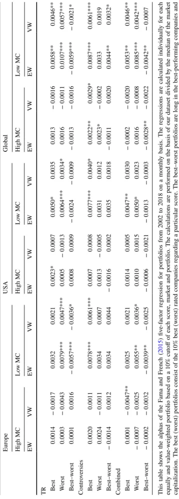
To further investigate whether the observed strong overper- formance of equally weighted portfolios with low TR ratings and high controversies scores is driven by company size, we divide our dataset at the median of the market capitalization and create new portfolios based on companies with high and low market capitalizations. Table 6 displays these portfo- lios based on a 10% cutoff for the European, US and global markets. From this table, it is apparent that the main results remain consistent, namely a significant outperformance of portfolios based on small companies with low TR score rat- ings as well as portfolios based on small companies with fewer controversies and therefore high controversies score.

It also can be seen from Table 6 that even the value-

weighted calculations based on firms with low market

capitalization mostly show significant and positive alphas

for controversies best, TR worst portfolios and ensure our

results.

Table 6

Alphas of eq uall y and v alue-w eighted 10% por tfolios: r eg ression based on high and lo w mar ke t capit alization This t able sho ws t he alphas of t he F ama and F renc h (

) fiv e-f act or r eg ression f or por tfolios fr om 2002 t o 2018 on a mont hl y basis. The r eg ressions ar e calculated individuall y f or eac h eq uall y and v alue-w eighted por tfolio based on a 10% cut off of eac h scor e, mar ke t and por tfolio. The calculations ar e per for med on t he basis of our dat ase t divided b y t he median of t he mar ke t capit alization. The bes t (w ors t) por tfolios consis t of t he 10% bes t (w ors t) r ated com panies r eg ar ding a par ticular scor e. The bes t–w ors t por tfolios ar e long in t he bes t-per for ming com panies and shor t in t he w ors t-per for ming ones. Mont hl y alphas ar e r epor ted upon. In or der t o es timate s tandar d er rors, w e use t he N ew ey and W es t (

) pr ocedur e ***, ** and * indicate a significance le vel of 1%, 5% and 10%

Eur ope U SA Global High MC Lo w MC High MC Lo w MC High MC Lo w MC EW VW EW VW EW VW EW VW EW VW EW VW TR  Bes t 0.0014 − 0.0017 0.0032 0.0021 0.0023* 0.0007 0.0050* 0.0035 0.0013 − 0.0016 0.0058** 0.0046**  W ors t 0.0003 − 0.0043 0.0079*** 0.0047*** 0.0005 − 0.0013 0.0064*** 0.0034* 0.0016 − 0.0011 0.0107*** 0.0057***  Bes t–w ors t 0.0001 0.0016 − 0.0057*** − 0.0036* 0.0008 0.0009 − 0.0024 − 0.0009 − 0.0013 − 0.0016 − 0.0059*** − 0.0021* Contr ov ersies  Bes t 0.0020 0.0011 0.0078*** 0.0061*** 0.0007 0.0008 0.0077*** 0.0040* 0.0022** 0.0029* 0.0087*** 0.0061***  W ors t 0.0024 − 0.0011 0.0034 0.0007 0.0013 − 0.0005 0.0031 0.0012 0.0023* − 0.0002 0.0033 0.0019  Bes t–w ors t − 0.0014 0.0012 0.0034 0.0044 − 0.0016 0.0002 0.0035 0.0018 − 0.0011 0.0020 0.0044** 0.0032* Combined  Bes t 0.0001 − 0.0047** 0.0025 0.0021 0.0014 0.0005 0.0047** 0.0030 − 0.0002 − 0.0020 0.0053** 0.0046**  W ors t − 0.0007 − 0.0025 0.0055** 0.0036* 0.0010 0.0015 0.0050* 0.0023 0.0016 − 0.0008 0.0085*** 0.0042***  Bes t–w ors t − 0.0002 − 0.0032 − 0.0039** − 0.0025 − 0.0006 − 0.0021 − 0.0013 − 0.0003 − 0.0028** − 0.0022 − 0.0042** − 0.0007

Rank‑weighted portfolios

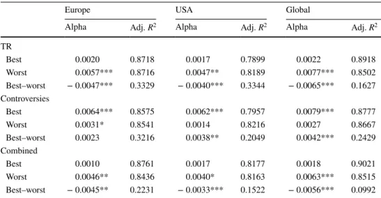
Table 7 displays best and worst rank-weighted portfolios based on a 10% cutoff for the European, US and global mar- ket. When considering these portfolios, nearly all returns of the best and worst portfolios are higher than with the cor- responding equally weighted strategies. Based on these cal- culations, the returns improve by up to 42.86%

for the best, by up to 32.24%

for the worst and by up to 84.28%

for the best-minus-worst portfolios, compared with the correspond- ing equally weighted portfolios. Note that rank-weighted portfolios also reveal a lower significance level in terms of p values, which indicates a real potential for investors.

On the one hand, there are a number of promising invest- ment strategies for investors who strongly attach importance to ESG scores. As we previously mentioned, the controver- sies score represents a huge potential for investors in particu- lar, and together with a rank-weighted portfolio strategy the corresponding alphas even increase, so this score describes a way in which to detect companies with a specific man- agement culture that apparently leads to higher future cash flows and therefore to higher and more significant alphas.

Surprisingly, companies with a high controversies score do not necessarily have a high ESG score. This noteworthy observation remains open for future research.

On the other hand, investors pursuing exactly the opposite strategy also benefit from rank weighting portfolios. This is particularly evident in the outperformance of the TR worst portfolios. Obviously, stronger weightings for firms with very low TR scores lead to significant overperformance, which can be traced back to a trade-off interpretation (see Aupperle et al. 1985). In summary, one can conclude that the rank weighting portfolios represent a useful tool for investors who wish to profit from ESG ratings either by investing in high-ranked companies or by investing in low-ranked firms.

Finally, to put it in a nutshell: buy the “saints” or invest in the “small sinners”.

Robustness checks

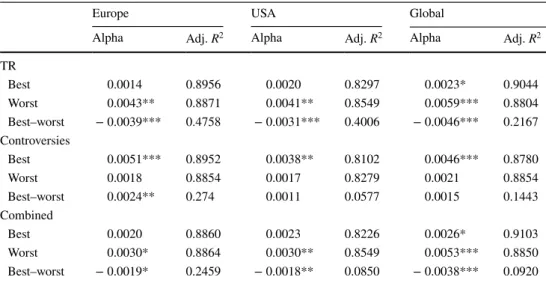
To check our results for robustness, we run some further regressions. First of all, we construct the equally weighted portfolios based on the 20% (instead of 10%) best and worst companies. Again we use the Fama and French (2015) five- factor regression model. The results are presented in Table 8 and indicate that all previous results remain materially the same for the 20% equally weighted selection, i.e., an out- performance of the controversies score best and the TR and combined score worst portfolios.

Moreover, with regard to the rank-weighted strategy, the 20% portfolios are also examined. Following the same

Table 7

Rank-weighted 10%

portfolios: regressions based on the three observed markets

This table shows the results of the Fama and French (2015) five-factor regression for portfolios from 2002 to 2018 on a monthly basis. The regressions are calculated individually for each rank-weighted portfo- lio based on a 10% cutoff of each score, market and portfolio set. The best (worst) portfolios consist of the 10% best (worst) rated companies regarding a particular score. The best–worst portfolios are long in the best-performing companies and short in the worst-performing ones. Monthly alphas and adj. R

are reported upon. In order to estimate standard errors, we use the Newey and West (1987) procedure

***, ** and * indicate a significance level of 1%, 5% and 10%

Europe USA Global

Alpha Adj. R

Alpha Adj. R

Alpha Adj. R

TR

 Best 0.0020 0.8718 0.0017 0.7899 0.0022 0.8918

 Worst 0.0057*** 0.8716 0.0047** 0.8189 0.0077*** 0.8502

 Best–worst − 0.0047*** 0.3329 − 0.0040*** 0.3344 − 0.0065*** 0.1627 Controversies

 Best 0.0064*** 0.8575 0.0062*** 0.7957 0.0079*** 0.8777

 Worst 0.0031* 0.8541 0.0014 0.8216 0.0027 0.8667

 Best–worst 0.0023 0.3216 0.0038** 0.2049 0.0042*** 0.2429

Combined

 Best 0.0010 0.8761 0.0017 0.8177 0.0018 0.9021

 Worst 0.0046** 0.8436 0.0040* 0.8163 0.0063*** 0.8515

 Best–worst − 0.0045** 0.2231 − 0.0033*** 0.1522 − 0.0056*** 0.0992

7

This displays the improvement in annual returns from 0.0693 to 0.0990 of the global controversies best portfolio.

8

This displays the improvement in annual returns from 0.0428 to 0.0566 of the Europe combined worst portfolio.

9

This displays the improvement in annual returns from 0.0280 to

0.0516 of the global controversies best–worst portfolio.

procedure, this leads to the results displayed in Table 9.

Also, in this case, all results of previous calculations remain approximately unchanged. Compared with the 20%

equally weighted portfolios, most of the alphas are higher.

For instance, we can observe an almost 20% increase in the alpha of the controversies best portfolio in the global market from 0.0046 to 0.0055, both being significant at a 1 % level.

As a next step, we divide our portfolios into bull and bear market periods to monitor how the portfolio strategies perform in different market phases. The results are shown in Table 10. The data suggest that the majority of the strategies work in bull markets. Moreover, one argument against this cannot be ignored: In our investigation period, there were mostly bullish phases and only a few bearish time periods,

Table 8

Equally weighted 20%

portfolios: regressions based on the three observed markets

This table shows the results of the Fama and French (2015) five-factor regression for portfolios from 2002 to 2018 on a monthly basis. The regressions are calculated individually for each equally weighted port- folio based on a 20% cutoff of each score, market and portfolio set. The best (worst) portfolios consist of the 20% best (worst) rated companies regarding a particular score. The best–worst portfolios are long in the best-performing companies and short in the worst-performing ones. Monthly alphas and adj. R

are reported upon. In order to estimate standard errors, we use the Newey and West (1987) procedure

***, ** and * indicate a significance level of 1%, 5% and 10%

Europe USA Global

Alpha Adj. R

Alpha Adj. R

Alpha Adj. R

TR

 Best 0.0014 0.8956 0.0020 0.8297 0.0023* 0.9044

 Worst 0.0043** 0.8871 0.0041** 0.8549 0.0059*** 0.8804

 Best–worst − 0.0039*** 0.4758 − 0.0031*** 0.4006 − 0.0046*** 0.2167 Controversies

 Best 0.0051*** 0.8952 0.0038** 0.8102 0.0046*** 0.8780

 Worst 0.0018 0.8854 0.0017 0.8279 0.0021 0.8854

 Best–worst 0.0024** 0.274 0.0011 0.0577 0.0015 0.1443

Combined

 Best 0.0020 0.8860 0.0023 0.8226 0.0026* 0.9103

 Worst 0.0030* 0.8864 0.0030** 0.8549 0.0053*** 0.8850

 Best–worst − 0.0019* 0.2459 − 0.0018** 0.0850 − 0.0038*** 0.0920

Table 9

Rank-weighted 20%

portfolios: regressions based on the three observed markets

This table shows the results of the Fama and French (2015) five-factor regression for portfolios from 2002 to 2018 on a monthly basis. The regressions are calculated individually for each rank-weighted portfo- lio based on a 20% cutoff of each score, market and portfolio set. The best (worst) portfolios consist of the 20% best (worst) rated companies regarding a particular score. The best–worst portfolios are long in the best-performing companies and short in the worst-performing ones. Monthly alphas and adj. R

are reported upon. In order to estimate standard errors, we use the Newey and West (1987) procedure

***, ** and * indicate a significance level of 1%, 5% and 10%

Europe USA Global

Alpha Adj. R

Alpha Adj. R

Alpha Adj. R

TR

 Best 0.0018 0.8884 0.0016 0.8214 0.0024* 0.9012

 Worst 0.0049*** 0.8853 0.0041** 0.8455 0.0069*** 0.8728

 Best–worst − 0.0042*** 0.4182 − 0.0035*** 0.4105 − 0.0056*** 0.1868 Controversies

 Best 0.0053*** 0.8838 0.0046** 0.8128 0.0057*** 0.8789

 Worst 0.0022 0.8772 0.0016 0.8311 0.0022 0.8804

 Best–worst 0.0021* 0.3409 0.0020 0.1333 0.0025** 0.2523

Combined

 Best 0.0015 0.8831 0.0022 0.8184 0.0023* 0.9056

 Worst 0.0041** 0.8738 0.0036** 0.8416 0.0058*** 0.8729

 Best–worst − 0.0036*** 0.2667 − 0.0025*** 0.1275 − 0.0045*** 0.1019

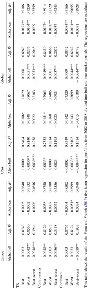
Table 10

Bull and bear mar ke t por tfolios This t able sho ws t he r esults of t he F ama and F renc h (

) fiv e-f act or r eg ression f or por tfolios fr om 2002 t o 2018 divided int o bull and bear mar ke t per iods. The r eg ressions ar e calculated individuall y f or eac h eq uall y w eighted por tfolio based on eac h scor e, mar ke t and por tfolio se t. The bes t (w ors t) por tfolios consis t of t he bes t (w ors t) r ated com panies r eg ar ding a par ticular scor e. The bes t–w ors t por tfolios ar e long in t he bes t-per for ming com panies and shor t in t he w ors t-per for ming ones. Mont hl y alphas and adj.

ar e r epor ted upon. In or der t o es timate s tandar d er rors, we use t he N ew ey and W es t (

) pr ocedur e ***, ** and * indicate a significance le vel of 1%, 5% and 10%

Eur ope U SA Global Alpha bull Adj.

Alpha bear Adj.

Alpha bull Adj.

Alpha bear Adj.

Alpha bull Adj.

Alpha bear Adj.

TR  Bes t 0.0003 0.8743 0.0005 0.8840 0.0000 0.8404 0.0186* 0.7629 0.0008 0.8943 0.0127** 0.9186  W ors t 0.0042** 0.8550 − 0.0002 0.9132 0.0030** 0.8140 0.0148 0.8067 0.0051*** 0.8276 0.0104** 0.9259  Bes t–w ors t − 0.0048*** 0.3944 − 0.0006 0.4646 − 0.0039*** 0.4258 0.0022 0.2103 − 0.0053*** 0.2048 0.0009 0.3559 Contr ov ersies  Bes t 0.0048** 0.8129 0.0058 0.8750 0.0033* 0.7553 0.0151* 0.7963 0.0049*** 0.8410 0.0107* 0.8914  W ors t 0.0003 0.8578 − 0.0007 0.8780 0.0000 0.8214 0.0160 0.7485 0.0001 0.8666 0.0130** 0.8729  Bes t–w ors t 0.0036** 0.3118 0.0052 0.5556 0.0023 0.1195 − 0.0023 − 0.0921 0.0037** 0.2072 − 0.0037 0.6243 Combined  Bes t 0.0003 0.8755 − 0.0004 0.8502 − 0.0002 0.8349 0.0142 0.7520 0.0009 0.8842 0.0084** 0.9166  W ors t 0.0033 0.8174 − 0.0051* 0.8999 0.0033** 0.8102 0.0143 0.8099 0.0044*** 0.8242 0.0101** 0.9055  Bes t–w ors t − 0.0039** 0.1933 0.0034 0.0940 − 0.0044*** 0.1514 − 0.0015 0.0100 − 0.0044*** 0.0748 − 0.0031 0.3928

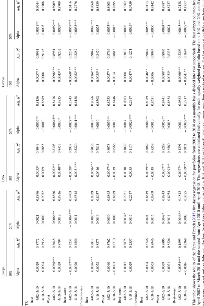
Table 11

Subper iod por tfolios This t able sho ws t he r esults of t he F ama and F renc h (

) fiv e-f act or r eg ression f or por tfolios fr om 2002 t o 2018 on a mont hl y basis divided int o tw o subper iods. The firs t subper iod dates fr om Apr il 2002 t o Mar ch 2010 and t he second fr om Apr il 2010 until Apr il 2018. The r eg ressions ar e calculated individuall y f or eac h eq uall y w eighted por tfolio based on a 10% and 20% cut off of eac h scor e, mar ke t and por tfolio se t. The bes t (w ors t) por tfolios consis t of t he 10% and 20% bes t (w ors t) r ated com panies r eg ar ding a par ticular scor e. The bes t–w ors t por tfolios ar e long in t he bes t-per for ming com panies and shor t in t he w ors t-per for ming ones. Mont hl y alphas and adj.

ar e r epor ted upon. In or der t o es timate s tandar d er rors, w e use t he N ew ey and W es t (

) pr oce - dur e ***, ** and * indicate a significance le vel of 1%, 5% and 10%

EuropeUSAGlobal 10%20%10%20%10%20% AlphaAdj. R2AlphaAdj. R2AlphaAdj. R2AlphaAdj. R2AlphaAdj. R2AlphaAdj. R2 TR  Best   4/02–3/100.00290.87720.00210.88960.0053*0.80490.0056**0.81560.0057**0.89910.0051**0.9044   4/10–3/180.00040.89360.00090.9052− 0.00090.8655− 0.00100.8689− 0.00080.9145− 0.00050.9108  Worst   4/02–3/100.0068***0.88480.0066**0.88860.0062**0.83080.00645**0.84180.0098***0.89810.0089***0.8909   4/10–3/180.00290.87940.00190.89160.0040**0.84530.0030*0.88350.0043**0.82320.0029*0.8709  Best–worst   4/02–3/10− 0.0057***0.3237− 0.0064***0.4403− 0.0028*0.2938− 0.0027**0.2843− 0.0060***0.2234− 0.0057***0.2416   4/10–3/18− 0.00260.4556− 0.00110.5545− 0.0051***0.5220− 0.0041***0.6138− 0.0052***0.2282− 0.0035***0.2776 Controversies  Best   4/02–3/100.0076***0.88170.0083***0.90390.0096***0.80360.0078***0.80660.0084***0.90470.0070***0.9068   4/10–3/180.00280.82730.00190.89570.00160.78110.00100.83020.0035**0.84200.00230.8439  Worst   4/02–3/100.00400.87620.00300.88950.0067**0.80780.0056**0.82330.0057**0.87660.0053**0.8903   4/10–3/18− 0.00030.87100.00020.8889− 0.00190.8566− 0.00130.8446− 0.00140.8815− 0.00130.8895  Best–worst   4/02–3/100.00170.38750.0034*0.29310.00100.1029− 0.00140.08830.00080.3832− 0.00020.3262   4/10–3/180.00290.25370.00150.27370.00330.1174− 0.0029***0.29170.0047**0.12710.0035*0.0759 Combined  Best   4/02–3/100.00040.87460.00210.88190.0059**0.80890.0063**0.80890.0046**0.90440.0058**0.9113   4/10–3/180.00650.89460.00150.8909− 0.00180.8559− 0.00100.8581− 0.00060.8984− 0.00060.9142  Worst   4/02–3/100.00390.88060.0048*0.88430.0067**0.82890.0058**0.84410.0088***0.89050.0084***0.8987   4/10–3/180.00210.82260.00110.89540.0093**0.85600.00180.88340.0033*0.83350.00210.8737  Best–worst   4/02–3/10− 0.0054***0.1895− 0.0046**0.1812− 0.0027*0.1291− 0.00140.0883− 0.0060***0.2206− 0.0045***0.2128   4/10–3/18− 0.00160.23680.00020.3785− 0.0059***0.3071− 0.0029***0.2917− 0.0041**0.1694− 0.0029**0.1757