Capital Structure Decisions and the Use of Factoring

Capital Structure Decisions and the Use of Factoring

Inauguraldissertation zur

Erlangung des Doktorgrades der

Wirtschafts- und Sozialwissenschaftlichen Fakultät der

Universität zu Köln

2013

vorgelegt von

Diplom-Mathematiker Alwin Stöter

aus

Leer

Referent: Prof. Dr. Thomas Hartmann-Wendels Korreferent: Prof. Dr. Dieter Hess

Tag der Promotion: 05.06.2013

Abstract

This thesis analyzes three research questions that belong to the field of corporate finance. The first and the second parts of this thesis examine predictions of the trade-off theory of capital structure.

This theory postulates that firms balance the benefits and costs of debt versus equity and as a result, choose target capital structures. The third research question analyzes the determinants of the decision of a firm to sell its accounts receivable to a factor.

According to the trade-off theory, the tax advantage of debt at the corporate level encourages firms with high marginal tax rates to bear more debt whereas the tax advantage of equity at the investor level leads to a lower debt ratio for firms with high personal tax rates. This thesis provides new evidence that taxes affect the capital structure choice of firms. Following the Graham methodology to simulate marginal tax rates, we find a statistically and economically significant positive relationship between the marginal tax benefit of debt (net and gross of investor taxes) and the debt ratio. A 10%

increase in the net (gross) marginal tax benefit of debt causes a 1.5% (1.6%) increase in the debt ratio, ceteris paribus.

Firms that face transaction costs may not adjust to their target capital structures immediately but

instead the adjustment takes a period of time. The speed of adjustment to target capital structure

has important implications for the relevance of the target capital structure for the firms’ choice of

financing. Recent studies show that a standard partial adjustment model with the debt ratio as the

dependent variable cannot distinguish between mechanical mean reversion and adjustment to target

capital structure. We propose a new approach that uses the net increase of debt as the dependent

variable and uses only ex-post information to estimate the target capital structure. Simulation

experiments show that this approach is mainly unaffected by mechanical mean reversion and hence able to provide a meaningful test for the target adjustment hypothesis. We estimate a speed of adjustment to target capital structure of 28% per year.

The third part of this thesis analyzes a firm’s decision of whether to accounts receivable internally,

use full-service factoring or enter into an in-house factoring contract. Our model is primarily based

on a theory of the firm that stresses a supplier’s need for financing, risk and financial flexibility. We

find that high-risk firms with a strong need for short-term financing and restricted access to bank

credit are more likely to use factoring. Larger firms typically prefer in-house factoring, whereas

smaller firms tend to rely on full-service factoring. The firm’s desire to attain independence from

banks plays an important role in decisions regarding factoring.

Acknowledgements

First of all, I would like to thank Thomas Hartmann-Wendels for supervising my thesis and provid- ing me advices and various comments to my work. I am also thankful to the second referee of my thesis Dieter Hess and to Heinrich Schradin for taking the chair of my disputation. I would like to thank the three of you for creating such a good atmosphere that led to the interesting discussion at the defense of my doctoral thesis.

I would also like to express my gratitude to Alexander Kempf and the German Research Foundation for granting me three years of funding for my thesis project and providing me an excellent program at the Graduate School of Risk Management.

My thanks also go to my colleagues at the graduate school for many hours of fruitful discussions and for having a really good time together during and after work. I wish you all the best for your careers and your social life.

I would like to thank my parents for standing always at my side and for providing me the encourage-

ment and support that I needed. My deepest thanks go to my girlfriend Miriam who enriched my

life with her warm refreshing way and her contagious smile. Thank you for listening to my research

problems and being part of my life.

Contents

Abstract iii

Acknowledgements v

Contents vii

List of Figures xi

List of Tables xiii

List of Abbreviations xv

List of Symbols and Variables xvii

1 Introduction 1

2 Tax Incentives and Capital Structure Choice: Evidence from Germany 7

2.1 Motivation . . . . 7

2.2 Measuring Tax Effects on Debt Usage . . . . 10

2.2.1 The Theoretical Model . . . . 10

2.2.2 The Simulated Marginal Tax Rate . . . . 11

2.2.3 The Empirical Model . . . . 13

2.3 Data and Summary Statistics . . . . 19

2.4 Taxes and Static Capital Structure . . . . 25

2.5 Robustness Checks . . . . 28

2.5.1 Issues Related to Data Selection . . . . 28

2.5.2 Taxes and Dynamic Capital Structure . . . . 30

2.5.3 Alternative Debt Ratio Definitions . . . . 32

2.6 Conclusions . . . . 33

3 How to Yield an Unbiased Estimate of the Speed of Adjustment to Target Capital Structure 35 3.1 Motivation . . . . 35

3.2 Measuring the Speed of Adjustment to Target Debt Ratios . . . . 38

3.3 Target Debt Ratio . . . . 44

3.3.1 Data and Summary Statistics . . . . 44

3.3.2 Target Debt Ratio Regressions . . . . 47

3.4 Partial Adjustment Regressions . . . . 49

3.4.1 Speeds of Adjustment Based on Simulated Samples . . . . 50

3.4.2 Speeds of Adjustment Based on Actual Data . . . . 55

3.5 Conclusions . . . . 56

4 Accounts Receivable Management and the Factoring Option: Evidence From a Bank- Based Economy 59 4.1 Motivation . . . . 59

4.2 The Determinants of Accounts Receivable Management . . . . 62

4.2.1 Transaction Costs . . . . 62

4.2.2 Economies of Scale . . . . 64

4.2.3 Financial Needs . . . . 64

4.2.4 Risk / Financial Health . . . . 66

4.2.5 Financial Flexibility . . . . 67

4.2.6 Industry Sector . . . . 67

4.2.7 Full-Service Factoring vs. In-House Factoring . . . . 68

4.3 Data and Summary Statistics . . . . 68

4.4 Results . . . . 69

4.4.1 Univariate Results . . . . 70

4.4.2 Multivariate Results . . . . 72

4.4.3 Qualitative Results . . . . 78

4.5 Conclusions . . . . 80

4.6 Appendix: Descriptions of the Categorial Variables . . . . 82

Bibliography 86

List of Figures

2.1 Mean Values of Tax Variables Over Time . . . . 22

2.2 Cross-Sectional Distribution of the Marginal Tax Benefit of Debt . . . . 23

2.3 Panel Distribution of the Marginal Tax Benefit of Debt . . . . 24

List of Tables

2.1 The Structure of Panel Data . . . . 20

2.2 Summary Statistics . . . . 21

2.3 Static Debt Ratio Regressions . . . . 26

2.4 Changes in Debt Regressions . . . . 29

2.5 Dynamic Debt Ratio Regressions . . . . 31

3.1 Summary Statistics . . . . 46

3.2 Target Debt Ratio Regressions . . . . 48

3.3 Adjustment Speeds to the Target Capital Structure: Coin Flip Samples . . . . 51

3.4 Adjustment Speeds to the Target Capital Structure: Random Sample and Actual Data 54 4.1 The Determinants of Accounts Receivable Management . . . . 62

4.2 Summary Statistics of the Independent Variables . . . . 68

4.3 The Univariate Results . . . . 71

4.4 The Multinomial Logistic Regression Results . . . . 74

4.5 The Reasons to Use or Avoid Factoring . . . . 79

List of Abbreviations

AR(1) Auto-regressive process of first order

CFO Chief financial officer

CRSP Center for Research in Security Prices

EBIT Earnings before interest and taxes

EBT Earnings before taxes

FE Fixed effects

GDP Gross domestic product

I Interest

IT Information technology

MTR Marginal tax rate

OLS Ordinary least squares

Perc. Percentile

SIC Standard industry classification

SMTR Simulated marginal tax rate

SOA Speed of adjustment to target capital structure

Std. Dev. Standard Deviation

TDR Target debt ratio

UK United Kingdom

US United States of America

List of Symbols and Variables

Assets (A) Book Assets

α Benefit from the deferral of capital gains

BEN ^{N et} _EBIT Marginal net tax advantage of debt with the simulated marginal tax rate based on EBIT (see Section 2.2.3)

BEN ^Gross _EBIT Marginal gross tax advantage of debt with the simulated marginal tax rate based on EBIT (see Section 2.2.3)

BEN ^{N et} Marginal net tax advantage of debt with the simulated marginal tax rate based on EBT (see Section 2.2.3)

BEN ^Gross Marginal gross tax advantage of debt with the simulated marginal tax rate based on EBT (see Section 2.2.3)

BEN Represents both BEN ^Gross and BEN ^{N et}

Collateral Net property, plant and equipment/A

d Dividend payout ratio

Debt (D) Short term financial debt + long term financial debt

Debt issues Dummy variable that is equal to one if the firm has a positive deficit and issues more debt than book equity

Debt repurchases Dummy variable that is equal to one if the firm has a negative

deficit and repurchases more debt than book equity

Def Financial deficit defined as Nei + Ndi

Def/Assets Def/A

∆ First difference operator

Dr D/A

Dr ^∗ Target debt ratio

Equity (E) Book equity

Normally distributed random variable with mean 0 and variance equal to the variance of historical ∆T I

k Def/(D+E)

i Firm i

Med Industry median debt ratio

I(NEGEQ) Dummy variable equal to 1 if the firm has negative equity I(NODIV) Dummy variable equal to 1 if the firm does not pay dividends I(NOL) _EBIT Dummy variable equal to 1 if the firm has a tax loss carry forward

that is based on EBIT

I(Regulated) Dummy variable equal to 1 if the firm belongs to a regulated industry

I(RND) Dummy variable equal to 1 if the firm has missing RND I(Sensitive) Dummy variable equal to 1 if the firm belongs to a sensitive

industry

h Factor that accounts for the restricted deductability of taxable income at the municipality level

λ Estimate of the speed of adjustment to target capital structure

MTB (A-E+market equity/A)

MTR _Graham Graham’s marginal tax rate based on EBIT

µ Moving average of historical ∆T I

Ndi First difference of Debt

NDTS Depreciation/A

Nei First difference of book equity

Re/Assets Retained Earnings/A

RND Research and development expense/sales

ROA EBIT/A

Size Natural logarithm of sales, deflated by the implicit price deflator

t Time t

τ _c Corporate tax rate

τ _e Personal tax rate on equity income

τ _{f ed} Federal corporate tax rate

τ _{f ed,re} Top statutory tax rate for retained earnings

τ loc Local corporate tax rate

τ i Personal tax rate on interest income

θ Imputation credit of taxes paid at the corporate level that is allowed by the tax system

TI Taxable income

Z-score (3.3·EBIT + sales+1.4·retained earnings + 1.2·(current assets -

current liabilities))/A

Chapter 1 Introduction

Even after more than 50 years of research based on the irrelevance theorem of Modigliani and Miller (1958), basic questions of corporate finance remain unclear: How do firms choose the mixture of debt and equity? What are the determinants of alternative financing instruments, e.g. entering into a factoring contract versus usage of a bank credit?

Taking the Modigliani and Miller’s irrelevance assumptions as a starting point, the capital structure research developed theories that state that a firm’s decision between debt and equity has an influence on the value of the firm. The capital structure literature can be divided into two groups (1) theories that postulate that firms have target debt ratios and (2) theories that don’t predict the existence of targets. The static trade-off theory of capital structure argues that firms balance the benefits of debt (e.g., tax benefits) against the costs of debt (e.g., costs of financial distress) and choose target capital structures. The pecking order theory predicts that firms follow a pecking order of financing, i.e.

firms first use internal generated funds to finance investments and in case of a financing deficit or

surplus, prefer debt over equity (see Myers and Majluf (1984)). The market timing theory states that

firms issue and repurchase equity in times of opportunity, i.e. firms issue equity when the market

valuation of equity is high and repurchase equity when the market valuation of equity is low (see

Baker and Wurgler (2002)). Both, the pecking order theory and the market timing theory do not

predict the existence of target debt ratios. Although some progress has been made there is still a

need to test the empirical relevance of competing capital structure theories. ¹

The first part of this dissertation tests the static trade-off theory of capital structure. We examine if taxes, both at the corporate and the personal level, affect the debt ratios of German firms. We further analyze which other determinants are important for the financing choices of firms. The results of this analysis serve as a starting point for the subsequent examination of the speed of adjustment to target capital structure, as we use the determinants that are found to relate to the costs and benefits of debt as a proxy for the target debt ratio. The speed of adjustment to target capital structure measures how much of the gap between the initial debt ratio and the predicted target capital structure is offset each year. Simulation experiments show that previously estimated speeds of adjustment are largely biased by mechanical mean reversion. We provide an approach that can differentiate between mean reversion of debt ratios and real adjustment to a target capital structure.

The second part analyzes the firms’ policy choice of the accounts receivable management. Firms must decide whether to vertically integrate the management functions that are associated with the trade credit extension or to employ a specialized intermediary like a factor. We differentiate between internal management of all trade credit functions, internal management of the debt collection but externalizing of the other functions to a factor (in-house factoring) and outsourcing of all trade credit functions to a factor (full-service factoring). In our model, we focus on the examination of determinants that relate to a theory of the firm that stresses a supplier’s need for financing, risk and financial flexibility.

The basic research questions that are adressed in this dissertation can be summarized as:

1. Do corporate and personal taxes reliably influence capital structures of German firms? What other determinants affect the firms’ financing choice?

2. Do firms adjust their capital structures towards targets? If yes, how important is the deviation

1

For a comprehensive overview of the empirical capital structure research, see e.g., Graham and Leary (2011) and

Parsons and Titman (2008).

from the target debt ratio for the firms’ financing decisions?

3. What are the determinants of a firm’s decision to sell its accounts receivables to a factor?

In the second and the third chapter of this thesis, we analyze a firm’s choice between debt and equity financing. To model a firm’s financing decisions we pursue the following approach (see e.g., Byoun (2008) and Chang and Dasgupta (2009)). The retained earnings and investments of a firm are assumed to be exogenous. As the primary source of financing the firm uses its internally generated earnings. If the internally generated funds do not suffice to finance the growth of the firm’s assets, the firm must decide whether to issue equity or debt. If the retained earnings exceed the firm’s financial needs, the remaining amount must be used to either repurchase equity or debt.

We test if these decisions are made in accordance with the trade-off theory of capital structure.

Chapter 2 investigates the relationship between taxes and the capital structure of German firms. ² The interest payments on the firm’s debt are a tax-deductible expense at the corporate level whereas such a provision does not exist for equity. This unequal treatment of debt and equity by law provides a tax advantage of debt at the corporate level. However, investors who receive interest payments from debt pay higher personal taxes than investors who own shares of the firm. So at the investor level, the tax law favors payments that arise from a stake in the firm’s equity. The overall effect remains unclear and depends on the country specific tax law. We test if firms with a high tax benefit of debt use high debt levels and issue more net debt to benefit from the tax advantage of debt.

We use Graham’s expected marginal tax rate approach for the identification of tax effects on the capital structure decision (see Shevlin (1990), Graham (1996a) and Graham et al. (1998)). We simulate various paths of future taxable income along which marginal tax rates are calculated that account for the carry forward and backward rules. This procedure accounts for the fact that firms may report losses and in this case, the tax shield cannot be used immediately and will offset future positive taxable income. Furthermore, we circumvent the endogeneity problem due to the reverse causality between debt and taxes. Recent studies using dichotomous tax rates based on net operating

2

See Graham (2003) for a detailed overview of the taxes and capital structure literature.

losses or effective tax rates arrive at a negative relation between tax rates and debt usage because they do not adequately take this issue into account (see e.g., Byoun (2008) and Antoniou et al.

(2008)).

In Chapter 2, we provide the first empirical analysis that shows a significant positive relationship between the marginal tax benefit of debt and the debt ratio for German firms using the Graham methodology to estimate marginal tax rates. In the empirical model, we simultaneously examine the influence of various other determinants on a firm’s capital structure which are motivated by the existence of information asymmetries, bankruptcy costs and transaction costs. A 10% increase in the marginal tax benefit of debt at the corporate level (investor level) causes a 1.5% (1.6%) increase in the debt ratio, ceteris paribus. This positive relationship can also be found in various other specifications of the dependent variable like changes in debt levels or net increase of debt.

Overall, the findings of this chapter provide empirical support for the trade-off theory of capital structure as firms issue more debt and choose higher debt ratios if they have higher marginal tax rates and higher (lower) values for firm characteristics that relate to the benefits (costs) of debt . Chapter 3 examines if and how fast firms adjust their capital structure toward their targets. In the presence of significant adjustment costs, firms may not adjust to their target capital structures immediately. For example, if the financial deficit is not high enough to close the gap between the initial debt ratio and the target debt ratio, the adjustment process takes more than one year. The magnitude of the speed of adjustment gives an insight how important the deviation from target is for the firms’ financing decisions. However, the previous literature produces different speeds of adjustment that range from 7% in Fama and French (2002) to 34% in Flannery and Rangan (2006) per year. Simulation experiments show that these estimates are biased by mechanical mean reversion (see Chang and Dasgupta (2009)).

We provide an unbiased estimate of the speed of adjustment to target capital structure by using the

following estimation technique. First, we rely on the net increase of debt instead of the debt ratio as

the dependent variable. Second, we use only historical data to estimate the target debt ratio. Third, we separate the coefficients of the target debt proxy and the lagged debt ratio (debt ratio at time t − 1) and interpret the coefficient of the predicted target as the speed of adjustment to target capital structure. This procedure produces low spurious speeds of adjustment in simulated samples where firms follow random financing. We find that firms close 28% of the gap between the debt ratio at the beginning of the year and the target debt ratio. ³ Thus, our results show that the deviation from the target debt ratio is important for the financing decision of a firm in accordance with the trade-off theory.

In Chapter 4, we analyze the determinants of a firm’s account receivable management policy choices.

The majority of the inter-firm trade is not paid directly; instead the seller commonly offers the buyer a certain period of time for the payments of the delivered services or goods. Firms that offer trade credit to customers must decide how to operate and finance the accounts receivable, i.e. which of the trade credit functions are managed within the firm and which of the functions are externalized to an intermediary like a factor. We emphasize that it is important to account for the included services in the factoring contract. Despite of the fact that most of the firms use in-house factoring, the previous literature models the firms accounts receivable management choice as a decision between internal management and the use of full-service factoring (see Smith and Schnucker (1994) and Summers and Wilson (2000)). In our model, the firm decides between internal management of all trade credit functions, use of in-house factoring and entering into a full-service contract. Furthermore, we investigate the influence of variables that relate to theories that stress the supplier’s need for financing, risk and financial flexibility on the factoring decision. We find that firms rely either on in-house or full-service factoring to meet short term financing needs and to diversify their financial portfolio. The full insurance of potential bad debts and the potential increase of the equity ratio are also important reasons for the firm’s decision to use factoring. Large firms prefer in-house factoring, whereas small, growing firms appreciate the relief of accounting requirements that is provided by

3

Hovakimian and Li (2011) use a similar technique but rely on the debt ratio as the dependent variable. By

additionally deleting high debt ratios in the simulated samples and the real sample, they come to an unbiased estimate

of the speed of adjustment of 5-8%.

full-service factoring.

The structure of this dissertation is the following:

Chapter 2 investigates the relationship between taxes, both at the corporate and the personal level, and the debt-equity choice. Furthermore, we analyze the influence of other determinants that are motivated by the trade-off theory on the capital structure of firms. We find that firms with a higher tax benefit of debt issue more net debt and choose higher debt ratios. The coefficients of the control variables are statistically significant and have the correct signs as predicted by the trade-off theory.

Chapter 3 examines the speed of adjustment to target capital structure. We construct random samples in which firms do not follow target behavior to test which specification of the partial adjustment model produces a low spurious speed of adjustment in these samples. We show that partial adjustment models that rely on debt ratios as the dependent variable are largely biased by mechanical mean reversion. In a specification that uses the net increase of debt as the dependent variable, we find that it takes a firm two years on average to offset 50% of the deviation from the target debt ratio.

Chapter 4 analyzes the firm’s choice of whether to vertically integrate the management of the accounts receivable or externalize the trade credit functions to a factor. In a multinomial model, we test which firm characteristics increase the probability to use in-house factoring or full-service factoring. We find that firms with a large customer base that are in need of short-term financing are more likely to employ a factor. Furthermore, firms who seek to increase their equity ratio and want to gain independence from a house bank prefer to use in-house factoring or full-service factoring.

Firms that use in-house factoring differ from firms that rely on full-service factoring mainly in size.

Chapter 2

Tax Incentives and Capital Structure Choice: Evidence from Germany

2.1 Motivation

It is widely held that the interest deductability of debt at the corporate level encourages firms to use debt financing, whereas personal income taxation provides a tax advantage of equity at the investor level leading firms to use less debt. The overall effect remains unclear and depends on the country-specific tax law. In this chapter, we examine the relationship between taxes, at both the corporate and the personal level, and the capital structure decision of a firm. We use a unique panel data set of firms resident in Germany.

Researchers face two general problems when they want to examine the effect of taxes on a firm’s

capital structure choice. First, the lack of variation of statutory tax rates over time as well as in

the cross-section of firms makes it difficult to identify tax effects. Second, a simultaneity bias

might occur because firms that exhibit a high debt ratio have high interest payments which in turn

lower the tax base and hence decrease the marginal tax rate. Thus, a regression model that uses a

tax rate that is based on income after interest deduction leads to a spurious negative estimate of

the coefficient of the tax variable (see Graham et al. (1998)). Despite this endogeneity problem,

recent studies still use marginal tax rates based on income after interest payments and thus arrive at a negative relation between tax rates and debt usage (see e.g., Byoun (2008) and Antoniou et al.

(2008)).

It is widely accepted in the theory of finance that the marginal tax rate is the relevant tax variable for the analysis of tax effects on the financing decision of a firm (see King and Fullerton (1984)).

The marginal tax rate is defined as the present value of taxes that are paid on one additional unit of income earned today (see Scholes and Wolfson (1992)). As long as the unit of income is sufficiently small, the marginal tax rate can be viewed as the present value of taxes that is shielded by one additional unit of income paid out as interest.

Our identification strategy relies on Graham’s methodology to simulate marginal tax rates (see Shevlin (1990), Graham (1996a) and Graham et al. (1998)). The simulated marginal tax rate that is used in this chapter incorporates an important feature of the German tax code, namely the asymmetric treatment of gains and losses. Firms only pay taxes at the statutory rate as long as the taxable income is positive. In Germany, losses are allowed to be carried forward and backward in time. When the tax base of a firm is fully exhausted (e.g., because of high existing depreciation and interest payments) an additional unit of interest paid today does not shield taxes today; instead it shields taxes at the time in the future when the firm first generates positive taxable income again.

Despite the fact that a considerable proportion of firms report losses and hence cannot exploit the full amount of potential tax deductions (marginal tax rates are below statutory tax rates in 30% of our sample), researchers often neglect the dynamic features of the tax code (e.g., Booth et al. (2001)).

We simulate various paths of future taxable income along which marginal tax rates are calculated

that account for the carry forward and backward rules. Averaging these marginal tax rates should

mimic the managers’ expectations of the marginal tax rate. Plesko (2003) and Graham (1996b)

show that the marginal tax rate that is based on simulations is the best available approximation of

the ‘true’ marginal tax rate. In particular, it is superior to just using variables that are assumed to be

highly correlated with the marginal tax rates, such as statutory tax rates, dummies which indicate

whether a firm is reporting losses or trichotomus variables, as used, for example, in Byoun (2008) or Gropp (2002).

We circumvent the endogeneity problem as our measure of the marginal tax rate is based on income before the relevant financing decision. In the debt ratio analysis, we use marginal tax rates that are based on earnings before interest and taxes. Since the debt ratio represents debt issued in the current and in the past period, we add all interest back to taxable income. In the analysis of changes in debt, where we examine only the amount of debt that is issued (or repurchased) in the current period, we rely on marginal tax rates that are based on the earnings before taxes and after interest payments at the beginning of the period.

Although there is increasing evidence of tax effects on capital structure choices for US firms (see MacKie-Mason (1990), Graham (1996a), Graham (1999)), evidence outside the US is rare. Alworth and Arachi (2001) simulate marginal tax rates following the Graham methodology for a panel of Italian firms and find evidence that corporate and personal taxes affect the debt usage of Italian firms.

However they focus on the net increase of debt as the explanatory variable and do not show if taxes

also influence debt ratios. Since the marginal tax benefit of debt depends heavily on country-specific

tax laws, existing results from other countries cannot be directly transferred to Germany. Using the

variation of top local tax rates across municipalities, Gropp (2002) shows that local taxes influence

the capital structure choice of German firms. However, he neglects the dynamic features of the tax

code and the effect of federal and personal taxes. We incorporate the dynamic local and federal

German tax code to accurately estimate marginal tax rates and show that the marginal tax benefit of

debt has a statistically and economically significant and positive effect on the debt ratio of firms

resident in Germany, both at the corporate level and the investor level (i.e., including personal

income taxes). A significantly positive effect of taxes on the change in debt ratio and the net increase

of debt is also identified. Recent empirical capital structure studies argue that transaction costs deter

firms from adjusting to their optimal capital structures immediately (see e.g., Flannery and Rangan

(2006)). For instance, firms could be reluctant to exploit the full marginal tax advantage of debt in a

scenario in which they face issuing costs of debt that outweigh the additional tax advantage of debt.

As a robustness check, we use a partial adjustment model to account for transaction costs and to rule out dynamic endogeneity concerns. We still find a significantly positive effect of taxes on the debt ratio. Several additional robustness checks are performed, such as alternative specifications of the dependent variable.

The rest of the chapter is organized as follows. We present our identification strategy in Section 2.2.

Section 2.3 shows some summary statistics and investigates the variation of the simulated marginal tax rates. In Section 2.4, we discuss the main results of the chapter, which are tested for robustness in Section 2.5. Section 2.6 presents the conclusions of this chapter.

2.2 Measuring Tax Effects on Debt Usage

In this section, we explain the identification strategy for measuring tax effects on the debt-equity choice. First, we describe the theoretical background for the empirical analysis, then we explain the simulation procedure for the marginal tax rates, which is crucial for the empirical model that is illustrated in the last part of this section.

2.2.1 The Theoretical Model

In Germany (as in most other countries), interest payments are deductible from taxable income,

whereas such a deduction is not allowed for equity. This provides a tax advantage of debt at the

corporate level (Modigliani and Miller (1963)). However, if interest income is taxed at a higher

personal tax rate than income in the form of dividends or capital gains, investors will demand a

higher pre-tax return for debt investments than for equity investments. This leads to a tax advantage

of equity at the investor level. Miller (1977) states that, at the margin, the tax disadvantage of debt

at the investor level completely offsets the tax advantage at the corporate level; that is, tax-induced

optimal capital structures do not exist in equilibrium. Neutrality with respect to different finance

instruments played a central role in past major German tax reforms. Thus, Germany is an excellent country to test Miller’s hypothesis. We measure the marginal tax advantage of debt, net of personal taxes, as the difference between the after-tax value of a dollar invested in debt and a dollar invested in equity (see Miller (1977)):

(1 − τ _i ) − (1 − τ _c ) (1 − τ _e ) , (2.1) where τ _i is the personal tax rate on interest income, τ _c is the corporate tax rate and τ _e is the personal tax rate on equity income. The tax rate on equity income covers the tax systems that were inherent in Germany during the observation period. To separate the effect of corporate taxes and personal taxes, the above equation can be transformed to

τ _c − [τ _i − (1 − τ _c ) τ _e ] . (2.2)

So the net tax advantage of debt equals the tax advantage of debt at the corporate level τ c (gross tax advantage of debt) minus the tax disadvantage of debt at the personal level. As long as the term in the square brackets is positive, the net tax advantage of debt is smaller than the tax advantage of debt at the corporate level. The next section deals with the empirical measurement of the corporate tax rate τ _c .

2.2.2 The Simulated Marginal Tax Rate

It is often implicitly assumed that firms are profitable in every state of nature and hence, the

corporate tax rate τ _c is equal to the top statutory tax rate. However, this disregards the possibility

that firms report losses or that tax loss carry forwards exceed taxable income. In that case the carry

back and carry forward provisions of the German tax code must be considered and τ _c can vary

between 0 and the top statutory tax rate. For instance, consider a firm with a tax loss carry forward

in t and positive taxable income in t + 1 exceeding tax loss carry forward in the time t. For this

firm, an additional unit of income in t lowers the tax loss carry forward provision in t and thus leads

to additional tax payments in t + 1. Discounting the (additional) tax payments in t + 1 yields a

marginal tax rate below the top statutory tax rate. This view is consistent with the marginal tax rate (MTR) defined as the present value of current and future taxes to be paid on an extra unit of time t income. Our measure of the MTR has two essential properties. First, it incorporates important features of the German tax code, such as the treatment of net operating losses and non-debt tax shields. Second, it reflects managers’ expectations of the MTR at time t when the debt decision is made. To account for the ability to carry losses forward in time we derive a forecasted stream of taxable income. Following Shevlin (1990) and Graham (1996a) we use a random walk with drift model to forecast taxable income:

∆T I _i,t = µ _i,t + _i,t , (2.3)

where ∆T I is the first difference of taxable income, µ is the (at least 3 and at most 7-year) moving average of historical ∆T I , with the moving average restricted to being non-negative, and is a normally distributed random variable with mean 0 and variance equal to the variance of historical

∆T I . ¹ Blouin et al. (2010) argue that the random walk approach is flawed because it does not account for mean reversion in taxable income, thus leading to extreme paths of future taxable income. Instead, they propose a nonparametric approach where future income is forecasted by draws from bins of firms that are grouped by profitability and assets size. However, Graham and Kim (2009) argue that using firm-specific information is important and show that the nonparametric approach produces too centralized distributions of marginal tax rates within the bins. Comparing the distribution of marginal tax rates using the random walk approach with the distribution of perfect-foresight marginal tax rates, Graham and Kim (2009) find that the random walk approach performs very well in predicting marginal tax rates. They further develop an AR(1) process which outperforms the bin and the random walk model. However, as using an AR(1) process would markedly reduce our sample size and the performance differences are small, we rely on the random walk approach to forecast taxable income.

1

Graham (1996b) shows that setting the mean µ to 0 if it would be negative yields a better estimate of the ‘true’

marginal tax rate. To model potential differences between trade balance sheets and tax balance sheets, taxable income is

adjusted for latent taxes. The precise definition of taxable income depends on the choice of the dependent variable and

is provided in the next section.

When estimating the MTR for firm i at time t, we first use the random walk with drift model to forecast a path of taxable income for the years t + 1, ..., t + 20 (the allowed carry forward period at time t is assumed to be unlimited in this example). ² Along this path we calculate the present value of the tax bill from t − 1 through t + 20 (the allowed carry back period is assumed to be one year in this example). Then we add 1000 euro (the smallest unit of income in our database) to time t income and calculate the present value of the tax bill again. The difference between the two tax bills yields a single MTR for the specific path of taxable income. We run this procedure for 50 different paths of taxable income and compute the average of these single MTRs. ³ The output is the (expected) simulated MTR for firm i at time t. Averaging the marginal tax rates over the 50 different scenarios of future taxable income should reflect the managers’ expectations about the marginal tax rate. In the following, we call this tax rate the simulated marginal tax rate (SMTR).

2.2.3 The Empirical Model

The SMTR is not only the best available approximation for the ‘true’ marginal tax rate (see Graham (1996b) and Plesko (2003)), it also contains enough variation to identify tax effects. Furthermore, as our identification strategy does not solely rely on tax rate or tax system changes over time, other overlapping time effects should not induce a major bias. However, since the SMTR relies on pre-tax income, an endogeneity bias may occur. Consider a firm with a high initial marginal tax rate. The high tax advantage of debt encourages the firm to use interest payments to shield taxes. Since interest payments are deductible from taxable income, the pre-tax income decreases. Thus the probability increases that the firm does not pay taxes in every state of nature, which leads to a low marginal tax rate. Hence, a firm with a high tax advantage of debt has low (after financing) marginal tax rates but use a high level of debt. This phenomenon leads to a spurious negative relation in regressions of tax variables on the usage of debt.

We use two strategies to avoid this endogeneity problem. First, we examine debt ratios (book

2

We restrict the carry forward period to 20 years; loss carry forwards at t + 21, ... are negligible due to discounting.

3

Using more than 50 paths does not significantly alter the estimates of the average marginal tax rates.

financial debt, both short term and long term, divided by total book assets) and use SMTRs based on earnings after non-debt tax shields before interest deductions (EBIT). Given that debt ratios reflect cumulative historical financing decisions, all interest (I) has to be added back to pre-tax income (EBT) to eliminate the simultaneity bias. Second, we investigate incremental financing choices, mostly used in past tax research, measured by the change in debt ratio (the first difference of debt divided by total book assets) as one specification and the net increase of debt (the first difference of debt, the difference divided by lagged total book assets) as another specification. ⁴ To circumvent simultaneity in these specifications we use lagged SMTRs based on earnings after non-debt tax shields and after interest payments (EBT), so that the tax variable is calculated before the time t financing decision is made but after historical financing choices.

Studying debt ratios has two drawbacks with respect to the incremental debt analysis. First, tests based on current financing decisions should have greater power since debt ratios contain aggregate past financing decisions. Second, no (implicit) assumption of an optimal capital structure is needed (more on that in Section 2.5.2). However, balance sheet data contain no information about actual security issues. The difference of book debt in consecutive years can be 0 or even negative (if the firm is paying down debt) for a high marginal tax rate firm, but this does not mean for sure that tax incentives are irrelevant for this firm. Instead, it could be the case that this firm is simply not in need of external funds (see Graham (1999)). Additionally, statistical and economic significance of taxes for the incremental financing choice cannot be carried over to debt ratios. Since most of the empirical capital structure research tries to explain existing debt ratios rather than incremental financing decisions, we focus on the debt ratio analysis. We address the above caveats as we also use incremental debt as the dependent variable in Section 2.4 and a partial adjustment model to cover dynamic effects in Section 2.5.

4

See Appendix A for details on the variable construction.

The Gross Tax Advantage of Debt

German firms pay corporate taxes at the federal level and local taxes at the municipality level, which were deductible from taxable income at the federal level until 2007. The local tax rate is calculated as the product of a base rate, which is constant through municipalities and changed once in the observation period, and a multiplicative coefficient, which differs among municipalities. Since we have no information about the locations of the firms in our sample and the key to which taxes are allocated among different locations, we use the average multiplicative coefficient of the Federal Statistical Office (Statistisches Bundesamt). ⁵ Interest payments are fully deductible at the federal level, but only partially deductible (most of the sample years, 50%) at municipality level. We therefore implement a multiplicative factor h which corrects for this special feature of the German tax code and the fact that local taxes have not been deductible at the federal level since 2008. Thus, the corporate tax rate τ _c can be written as

τ c = τ f ed + h · τ loc · (1 − τ f ed ) , (2.4)

where τ _{f ed} is the federal corporate tax rate and τ _loc is the local corporate tax rate. Before 2001, corporate profits in form of retained earnings were taxed at a higher rate than dividends, which provided partial relief from the double taxation of dividends at the corporate and personal level.

We use the corporate tax rate for retained earnings in our simulation method. ⁶ To account for uncertainty of income and the asymmetries in the local tax code, we multiply the local tax rate τ loc

by the SMTR divided by the top tax rate for retained earnings. ⁷ In a nutshell, the tax advantage of debt at the corporate level BEN ^Gross (gross of personal taxes) is calculated by

BEN ^Gross = SM T R + h · τ _loc · SM T R

τ _{f ed,re} (1 − SM T R) , (2.5)

5

See Gropp (2002) for an approach using cross-sectional variation in the multiplicative coefficient to identify tax effects.

6

The results remain essentially the same if we use a tax rate weighted by the dividend payout ratio.

7

In Germany, it is permitted to carry local tax losses forward in time (with the duration and volume being equal to that

of federal tax losses), but not backward in time (see section 10a of the German Trade Tax Act (Gewerbesteuergesetz)).

where τ _{f ed,re} is the top statutory tax rate for retained earnings.

The Net Tax Advantage of Debt

To derive BEN ^{N et} , the tax advantage of debt net of personal taxes, we insert the gross tax advantage of debt into Equation (2.1):

BEN ^{N et} = (1 − τ _i ) − 1 − BEN ^Gross

(1 − τ _e ) . (2.6)

The tax rate on interest income τ _i equals the personal income tax rate during the period under review.

The taxes paid on equity income depend on the tax system and on the fraction of income paid out as dividends. Let d denote the dividend payout ratio, α the benefit from the deferral of capital gains and θ the imputation credit of taxes paid at the corporate level that is allowed by the tax system (see King (1977)). ⁸ We assume that the ‘marginal investor’ is in the highest tax bracket and that capital gains are taxable. ⁹ Since dividends and capital gains are taxed at the same rate τ _d in Germany, we can write

(1 − τ _e ) = dθ (1 − τ _d ) + (1 − d) (1 − ατ _d ) . (2.7)

From 1971 to 2008, the period under review, there existed three different tax systems. From 1971 to 1976, a classical tax system similar to that in the US with different corporate tax rates for dividends and retained earnings was in place. This tax system was followed by a full imputation system, again with a split rate of corporate tax. In 2001, the government introduced a shareholder relief system, under which only half of the equity income was taxed at the personal level. These different tax systems are reflected in the parameter θ and in the tax rate τ _d .

In our capital structure analysis throughout this chapter, we run each regression model, first, by using the BEN ^Gross variable as one specification, which only represents the tax advantage of

8

In the empirical analysis the dividend payout ratio is lagged one year to avoid a simultaneity bias.

9

We run the analysis with tax-free capital gains, but the results are qualitatively the same.

debt at the corporate level, and second, by using the BEN ^{N et} variable as another specification, which also incorporates investor taxes. Hereafter, we refer to BEN ^Gross and BEN ^{N et} as the BEN variables.

Control Variables

We control for various other factors beside the tax advantage of debt that influence financing decisions. DeAngelo and Masulis (1980) argue that the tax shield that is produced by interest deductions competes with non-debt tax shields like depreciation allowances. However, the BEN variables already incorporate non-debt tax shields, since the taxable income used for the tax rate calculations is based on pre-tax income after depreciation. Within the simulation of the marginal tax rate, non-debt tax shields are modeled according to the random walk with drift model described in Section 2.2.2. ¹⁰

The trade-off theory postulates that managers balance the benefits and costs of debt when they make financing decisions. However, the costs of debt are difficult to measure directly. For example, financial distress costs are difficult to separate from economic distress costs (which occur due to other reasons than high debt ratios and thus are irrelevant for the financing decision) and researchers are still searching for accurate estimates of financial distress costs for single firms (see Graham and Kim (2009), Korteweg (2010) and Van Binsbergen et al. (2010)). Following Graham et al. (1998), we use two variables for the ex post financial distress costs of debt depending on firm characteristics.

First, we include the modified Altman’s Z-score, which is measured as (see Altman (1968) and MacKie-Mason (1990)):

Z-score = 3.3EBIT + Sales + 1.4Retained Earnings + 1.2Working Capital

Total Assets . (2.8)

10

See Graham et al. (2004) for other non-debt tax shields such as employee stock options that relate to the capital

structure decisions of US firms.

We expect the corresponding coefficient to have a negative sign. The lower the Z-score, other things being equal, the more likely the firm is in financial distress, leading to deterioration of equity.

Second, we use I(NEGEQ), a dummy variable which is equal to 1 if equity is negative. For the same reason as noted above, I(NEGEQ) should be positively related to debt usage. Another variable indicates whether an industry is likely to suffer from ex ante financial distress costs. When firms that produce unique products enter into liquidation, they impose large costs on suppliers and customers (e.g., lack of repair service and spare parts). A high proportion of debt in the capital structure induces a high probability of liquidation, leading to high (expected) financial distress costs, e.g.

because customers may be reluctant to buy products of these firms. Consequently, these firms should use less debt than other firms, ceteris paribus. To gauge product uniqueness, we follow Titman (1984) and use a dummy variable I(Sensitive) which is equal to one if the firm is in a industry with high assumed financial distress costs. These industries are identified by the SIC codes between 3400 and 4000.

The effects of profitability on usage of debt are ambiguous. On the one hand, from the perspective of the trade-off theory, profitable firms should use a high amount of debt to shield taxes since they are unlikely to go bankrupt. An additional argument for profitable firms using higher debt ratios than unprofitable firms is given by the free cash flow hypothesis stated by Jensen (1986). This theory claims that interest payments discipline managers to not divert funds into their own pockets (e.g., through empire building) and thus, large interest payments mitigate the moral hazard problems between managers and stockholders. On the other hand, according to the pecking order theory (see Myers and Majluf (1984)), firms use first internal equity and when internal funds do not suffice, debt financing is preferred over equity financing. Thus, this theory implies that profitable firms use less debt in their capital structure since they are more likely to be not in need of external funds. We measure profitability by the variable ROA, which is defined as operating cash flow divided by total assets.

Amihud and Murgia (1997) show that dividends are informative about values of listed German

companies (although dividends are not tax-disadvantaged by German tax law). Thus, it could be argued that dividend-paying firms do not suffer from a large ‘lemons’ premium when issuing new equity. Vice versa, firms that do not pay dividends may be subject to large informational asymmetries, perhaps causing them to prefer debt over equity financing (see Sharpe and Nguyen (1995)). To capture the amount of information asymmetries with respect to the information content of dividends, a no dividend dummy I(NODIV) is included into the regression. We expect the sign of I(NODIV) to be positively related to the use of debt. Moreover, regulated firms are likely to be less levered because the regulatory agency may provide investors with relevant information and thus reduce signaling costs (see MacKie-Mason (1990)). We therefore include the industry dummy variable I(Regulated) for the energy and water supply industry and the railroad industry.

Large firms are likely to be well diversified and should therefore face low ex ante costs of financial distress. In addition, large firms often have lower informational costs and lower transaction costs when issuing securities. Therefore, larger firms are more likely to have a high debt ratio, other things being equal. We measure Size by the natural logarithm of sales, where sales, expressed in million euro, are deflated by the implicit price deflator. ¹¹ Firms with a high proportion of Collateral should borrow on favorable terms and are expected to issue more debt. Collateral is defined as net property, plant and equipment divided by total assets. Year dummies are also included to control for unobserved time effects such as macroeconomic effects.

2.3 Data and Summary Statistics

Our empirical analysis is based on the balance sheet database Unternehmensbilanzstatistik of the Deutsche Bundesbank; it is one of the most comprehensive databases for German non-financial firms. The database was established for the Deutsche Bundesbank’s rediscount business in 1971.

The Bundesbank was required to purchase bills that were backed by parties known to be solvent (see Stöss (2001)). German firms used as collateral in this business had to submit their complete

11

As a robustness check, we replace sales by total assets; the results are qualitatively unchanged.

Table 2.1: The Structure of Panel Data

The sample consists of all non-financial corporations in the Unternehmensbilanzstatistik of the Deutsche Bundesbank with at least three consecutive observations. The listed variables are winsorized at the 1st percentile and the 99th percentile. Total assets and Sales are expressed in million euro and are deflated by the implicit price deflator. Z-score is the modified Altman’s (1968) Z-score. I(NEGEQ) is a dummy variable that is equal to 1 if the firm has negative equity.

I(NOL)

is a dummy variable that is equal to 1 if the firm has an EBIT based tax loss carry forward (calculated within the simulation of the marginal tax rate based on EBIT).

Year Mean Std. Dev. 25th Perc. Median 75th Perc.

Employees 1975 567.80 2056.54 15.00 75.00 300.00

1985 229.47 1399.85 4.00 21.00 75.00

1995 236.46 1231.90 12.00 32.00 93.00

2005 322.82 1338.26 17.00 51.00 169.00

Total assets 1975 19.20 68.27 0.57 1.80 6.67

1985 9.10 47.60 0.25 0.61 2.00

1995 10.32 48.88 0.33 0.78 2.50

2005 31.81 89.11 1.06 3.34 14.42

Sales 1975 23.06 75.10 1.09 3.23 10.80

1985 12.79 56.79 0.55 1.38 4.18

1995 13.27 55.92 0.70 1.72 4.81

2005 35.75 94.25 2.04 6.03 20.93

Z-score 1975 2.54 1.73 1.52 2.20 3.07

1985 2.89 1.82 1.75 2.56 3.59

1995 2.73 1.75 1.57 2.43 3.51

2005 2.79 1.79 1.60 2.57 3.66

I(NEGEQ) 1975 0.25 0.43 0.00 0.00 1.00

1985 0.29 0.45 0.00 0.00 1.00

1995 0.12 0.33 0.00 0.00 0.00

2005 0.04 0.19 0.00 0.00 0.00

I(NOL)

1975 0.16 0.37 0.00 0.00 0.00

1985 0.08 0.27 0.00 0.00 0.00

1995 0.13 0.34 0.00 0.00 0.00

2005 0.13 0.34 0.00 0.00 0.00

financial statements to the Bundesbank to check their creditworthiness; these financial statements are collected in the Unternehmensbilanzstatistik. Thus, missing data are not a big issue for the database.

The database consists of annual data for over 100,000 corporations (mostly limited liability compa-

nies) over the period from 1971 to 2008. The simulation method of the marginal tax rate requires at

least three consecutive observations. This requirement leads to 623,780 observations (86,173 firms)

for the years 1973 to 2008.

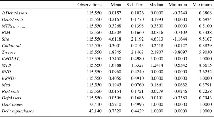
Table 2.2: Summary Statistics

The sample consists of all non-financial corporations in the Unternehmensbilanzstatistik of the Deutsche Bundesbank from the years 1973 to 2008 with at least three consecutive observations. Debt is short term financial debt plus long term financial debt. BEN

is the marginal net tax advantage of debt with the simulated marginal tax rate based on EBIT (see Section 2.2.3). BEN

is the marginal gross tax advantage of debt with the simulated marginal tax rate based on EBIT (see Section 2.2.3). BEN

is the marginal net tax advantage of debt with the simulated marginal tax rate based on EBT. BEN

is the marginal gross tax advantage of debt with the simulated marginal tax rate based on EBT. ROA is defined as operating income after depreciation divided by total assets. Size is the natural logarithm of sales, deflated by the implicit price deflator. Collateral is net property, plant and equipment divided by total assets.

Z-score is Altman’s (1968) modified Z-score. I(NEGEQ) is a dummy variable that is equal to 1 if the firm has negative equity. I(NODIV) is a dummy variable that is equal to 1 if the firm does not pay dividends. I(Regulated) is a dummy variable that indicates if the firm belongs to a regulated industry. I(Sensitive) is a dummy variable that indicates if the firm belongs to a sensitive industry. The listed variables are winsorized at the 1st percentile and the 99th percentile.

Observations Mean Std. Dev. Median Minimum Maximum

Debt/Assets 623780 0.3059 0.2359 0.2776 0.0000 0.8804

BEN

623780 -0.0100 0.1078 0.0290 -0.4477 0.1064

BEN

623780 0.4691 0.1351 0.5253 0.0000 0.5937

BEN

536139 -0.0404 0.1287 0.0158 -0.4477 0.1064

BEN

536139 0.4316 0.1578 0.4931 0.0000 0.5937

ROA 623780 0.0738 0.1125 0.0585 -0.3277 0.5020

Size 623780 0.9656 1.8135 0.7739 -3.5870 6.1868

Collateral 623780 0.2043 0.2074 0.1349 0.0000 0.8871

Z-score 623780 2.7872 1.7907 2.4791 -0.3969 10.3764

I(NEGEQ) 623780 0.1415 0.3485 0.0000 0.0000 1.0000

I(NODIV) 623780 0.7520 0.4319 1.0000 0.0000 1.0000

I(Regulated) 623780 0.0135 0.1153 0.0000 0.0000 1.0000

I(Sensitive) 623780 0.2313 0.4217 0.0000 0.0000 1.0000

Since 1998, the number of balance sheets per year in the sample has decreased by about two-thirds, reaching a level of approximately 20,000 in 2008. This drop is connected to the fact that the discount credit facility in the context of bill-based lending was not included in the European Central Bank’s set of monetary policy instruments (see Bundesbank (2001)). This implies that, since 1999, the requirements with respect to the creditworthiness of the companies to be included in the database were strengthened (Article 18.1 of the Statute of the European System of Central Banks). The reduced sample size leads to a reduction of the statistical power of the data set. Moreover, due to the collection mechanism, a certain quality bias may occur.

Table 2.1 presents statistics of selected variables that describe the structure and quality of the data

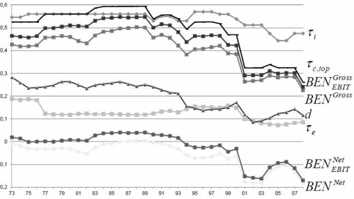
Figure 2.1: Mean Values of Tax Variables Over Time

This figure shows the mean annual values for several tax variables and the dividend payout ratio d over the years 1973−2008. τ

is the personal tax rate on interest income, which is equal to the top personal income tax rate. τ

is a combination of the top statutory federal and local tax rate (see Equation (2.4)). For details of the construction of t

, the personal tax rate on equity income, and BEN

(BEN

), the tax benefit of debt net (gross) of investor taxes, see Section 2.2.3.

set used in this study. The statistics of Employees, Sales and Total assets show that the data set

contains small, medium sized and large companies. Our analysis may be favored with respect to the

identification and the magnitude of tax affects if financially distressed firms are underrepresented in

the data set. We therefore provide statistics for the variables Z-score and I(NEGEQ) which indicate

if firms suffer from (ex post) financial distress. The distribution of the Z-score variable suggests

that the main part of the firms in the data set are financially healthy (75% of the Z-score values are

higher than 1.5). However, the mean values of I(NEGEQ) show that firms report negative equity

in a substantial part of the observations, which indicates that the data set contains also financially

distressed firms. The increase in the statistics of the Z-score and the variables that measure the

firms’ size and the decrease of the mean value of I(NEGEQ) from 1995 to 2005 reflect the change

in the collection mechanism after the beginning of the monetary union.

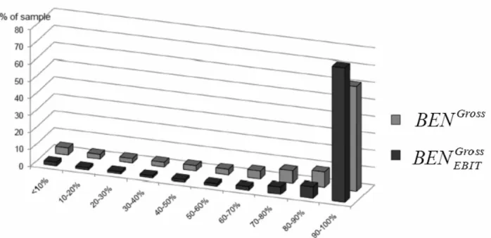
Figure 2.2: Cross-Sectional Distribution of the Marginal Tax Benefit of Debt

This figure presents the cross-sectional distribution of the variables of the marginal tax benefit of debt, gross of investor taxes. The BEN

variables are divided by the top statutory tax rate to fade out time-series changes. The construction of the BEN

variables is described in Section 2.2.3.

Central to the identification strategy in this chapter is that the sample contains enough firms with pre-tax losses. Table 2.1 reports statistics of I(NOL) _EBIT , a dummy variable which is equal to one if the firm has accumulated a tax loss carry forward based on EBIT. As our main analysis studies the effect of taxes on debt ratios that cover all debt issues in the past that result in interest payments today, tax losses that are based on EBIT are accumulated within the simulation of the marginal tax rate to circumvent endogeneity problems. The amount of firms with tax loss carry forwards that are based on EBIT (13%) remains unchanged from 1995 to 2005. To examine a possible selection bias, we run additional robustness checks (see Section 2.5.1).

Table 2.2 reports some summary statistics for the dependent and explanatory variables. To remove

outliers from the sample, variables are winsorized at the 1st percentile and the 99th percentile,

respectively. The debt ratio has a sample mean (median) of 30.59% (27.76%) with a standard

deviation of 23.59%. All variables exhibit substantial variation. In the following, we analyze the

variation in the BEN variables in more detail, which is crucial for the identification of tax effects.

Figure 2.3: Panel Distribution of the Marginal Tax Benefit of Debt

This figure shoes the panel distribution of variables of the marginal tax benefit of debt. The construction of the BEN variables, net and gross of investor taxes, can be found in Section 2.2.3.

Figure 2.1 shows the time variation in the mean values of the tax variables. The mean values of the BEN variables exhibit some time-series variation. Most of the time-series variation stems from tax reforms which changed the top statutory corporate tax rates and personal tax rates. The remaining variation in the BEN ^Gross variables over time can be mainly explained by the change in the treatment of tax losses with regard to carry forward and carry back provisions. The BEN ^{N et} variables additionally vary with the dividend payout ratio. The tax advantage of debt slightly increases 1983 due to the fact that interest payments were the first time deductible from the local tax base. The two larger declines in 2001 and 2008 can be mainly explained by the decrease in top federal corporate tax rates.

The fact that the tax rate for equity payments is markedly smaller than the tax rate for interest

payments explains the wide spread between the gross tax advantage of debt and the net tax advantage

of debt. Since we use the top statutory tax rate for the marginal personal income tax rate, the net tax

advantage of debt can be interpreted as a lower bound.

Figure 2.2 presents the cross-sectional variation in the BEN ^Gross variables. BEN ^Gross values are divided by the top statutory tax rate to blank out time-series changes in the top statutory tax rates.

The BEN variables based on EBIT measure the tax advantage of the first euro of interest payments, whereas the BEN variables based on EBT measure the tax advantage of the last euro of interest payments. Since interest payments lower taxable income, the values for the tax benefit of debt based on EBIT exhibit less variation than the tax rates based on EBT and a higher percentage of EBIT based tax benefits are equal to the top statutory tax rate (70% versus 60%). ¹²

Figure 2.3 shows that our measure of the tax benefit of debt exhibits substantial variation when both the time-series and cross-sectional dimension are considered. Once personal taxes are taken into account, the sample distribution of the gross tax benefit of debt moves to the left. Thus, the higher personal tax rate on interest income with respect to equity income reduces the tax benefit of debt at the corporate level. Comparing the tax benefit of debt before and after interest, the Figures 1−3 reflect the endogenous relation between debt and the marginal tax rate.

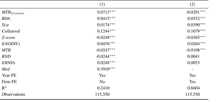
2.4 Taxes and Static Capital Structure

Table 2.3 presents the main results of our estimations. Throughout this chapter (unreported) year dummies are included to control for any unmodeled time effects. Standard errors are robust to within firm correlation, as we cluster the standard errors by firm, and are robust to heteroscedasticity by using the technique of White (1980). ¹³ Columns (1) and (2) of Table 2.3 show the estimates for the dependent variables using pooled OLS, with Column (1) including the net tax benefit of debt and Column (2) covering the gross tax benefit of debt. ¹⁴ The tax benefit of debt has a statistically and economically significant and positive effect on the debt ratio, both gross and net of personal taxes. A 10% increase in the marginal tax benefit of debt follows a 1.5-1.6% increase in the debt

12

The cross-sectional variation shown in Figure 2.2 changes only slightly over time.

13

See Petersen (2009) for a detailed analysis which estimation technique for the standard errors should be used in finance panel data.

14

Since the debt ratio is winsorized we also run a Tobit regression. The results essentially remain the same.