Logic II
Markus Lohrey
Universit¨at Siegen
Summer 2021
General comments
Informations concerning the lecture can be found at
http://www.eti.uni-siegen.de/ti/lehre/ss21/logikii/:
◮ current version of the slides
◮ links to the videos
◮ exercise sheets Literature:
◮ Sch¨oning: Logik f¨ur Informatiker, Spektrum Akademischer Verlag 2013
(English Edition: Logic for Computer Scientists, Birkh¨auser 2008)
◮ Ebbinghaus, Flum, Thomas: Einf¨uhrung in the mathematische Logik, Spektrum Akademischer Verlag
(English Edition: Mathematical Logic, Springer 1994) The tutorialswill be organized by Louisa Seelbach.
Recapitulation from the lecture GTI
Definition (recursively enumerable)
A languageL⊆Σ∗ is recursively enumerable, if there is an algorithm with the following properties:
For x ∈Σ∗ we have:
◮ If x ∈L, then the algorithm terminates with inputx.
◮ If x 6∈L, then the algorithm does not terminate with inputx.
German term: semi-entscheidbar.
Lemma
A languageL⊆Σ∗ is recursively enumerable if and only if there is a computable total function f :N→Σ∗ withL={f(i)|i ∈N}.
Recapitulation from the lecture GTI
Definition (decidable and undecidable)
A languageL⊆Σ∗ is decidable, if there is an algorithm with the following properties: for all x ∈Σ∗ we have:
◮ If x ∈L, then the algorithm terminates on inputx with output “Yes”.
◮ If x ∈/L, then the algorithm terminates on inputx with output “No”.
A languageL⊆Σ∗ is undecidable, ifLis not decidable.
Theorem
A languageL⊆Σ∗ is decidable if and only if Land Σ∗\Lare both recursively enumerable.
Recapitulation from the lecture Logik I
We assume the following notions/definitions from Logik I
◮ formulas of predicate logic (formulan der Pr¨adikatenlogik) Example: G =∀x∃y(P(x,f(y))∧ ¬Q(g(z,x)))
◮ sentence = formulas without free variable (Aussagen) Example: F =∀x∃y(P(x,y)∧ ¬P(f(x),x))
◮ structure (Struktur)A= (UA,IA), whereUA is the universe of the structure andIA is the interpretation function (we write fA=IA(f)).
Example: UA =N,fA(n) =n2,PA ={(n,m)|n<m}.
◮ StructureA is suitable (passend) for a formulaF. Example: Ais suitable for F, but not suitable forG.
◮ A |=F:F evaluates to 1 (= true) in the structure A.
Whenever we write A |=F, we implicitly assume that Ais suitable for F.
Recapitulation from the lecture Logik I
A formula F of predicate logic is:
◮ satisfiable, if there is a structureA such thatA |=F (F is true in the structure A).
◮ valid, ifA |=F holds for every structureA. Corollary of Gilmore’s theorem
The set of all unsatisfiable formulas of predicate logic is recursively enumerable.
Corollary
The set of all valid formulas of predicate logic is recursively enumerable.
Proof:F is valid if and only if ¬F is unsatisfiable.
Undecidability in predicate logic
We want to prove the following important result:
Church’s theorem
The set of valid formulas of predicate logic is undecidable.
Corollary
The set of satisfiable formulas of predicate logic is not recursively enumerable.
Proof:The set of unsatisfiable formulas of predicate logic is recursively enumerable.
If the set of satisfiable formulas of predicate logic would be recursively enumerable, then it would be decidable.
Hence, also the set of unsatisfiable (and hence the set of valid) formulas would be decidable.
Register machines
We prove Church’s theorem by a reduction from the halting problem for register machine programs.
Let R1,R2, . . . be (names for) registers.
Intuition: Every register stores a natural number.
A register machine program (RMP for short) P is a sequence of
instructionsA1;A2;. . .;Al, whereAl is the STOP instruction, and for all 1≤i ≤l−1 the instruction Ai is of one of the following types:
◮ Rj :=Rj + 1 for some 1≤j ≤l
◮ Rj :=Rj −1 for some 1≤j ≤l
◮ IFRj = 0 THENk1 ELSE k2 for some 1≤j,k1,k2≤l.
Note: We assume that only the registers R1, . . . ,Rl are used in an RMP withl instructions. This is no restriction.
Register machines
A configurationof P is a tuple (i,n1, . . . ,nl)∈Nl+1 with 1≤i ≤l. Intuition: i is the number of the instruction that is executed next andnj is the current content of register Rj.
For configurations (i,n1, . . . ,nl) and (i′,n′1, . . . ,n′l) we write (i,n1, . . . ,nl)→P (i′,n1′, . . . ,nl′)
if and only if 1≤i ≤l−1 and one of the following cases holds:
◮ Ai = (Rj :=Rj + 1) for some 1≤j ≤l,i′=i+ 1,n′j =nj + 1, n′k =nk for k 6=j.
◮ Ai = (Rj :=Rj −1) for some 1≤j ≤l,i′=i+ 1,nj =nj′ = 0 or (nj >0,n′j =nj −1), and n′k =nk for k 6=j.
◮ Ai = (IF Rj = 0 THENk1 ELSE k2) for some 1≤j,k1,k2 ≤l, n′k =nk for all 1≤k ≤l,i′ =k1 ifnj = 0, i′ =k2 ifnj >0.
Register machines
Example: The following RMPP simulates R1 :=R1+R2: IF R2 = 0 THEN 5 ELSE 2;
R1 :=R1+ 1;
R2 :=R2−1;
IF R1 = 0 THEN 1 ELSE 1;
STOP
More precisely: For all numbers n1,n2 we have
(1,n1,n2,0,0,0) →∗P (5,n1+n2,0,0,0,0).
Register machines
The configuration is (1,0, . . . ,0) (all register contain 0, first instruction is executed) is also called starting configuration.
We define
HALT ={P |P =A1;A2;. . .;Al is a RMP with l instructions, (1,0, . . . ,0)→∗P (l,n1, . . . ,nl) forn1, . . . ,nl ≥0}. Register machine programs exactly correspond to GOTO-programs from the GTI lecture.
In GTI we proved that Turing machines and GOTO-programs can simulate each other.
Register machines
Since the halting problem for Turing machines starting with the empty tape (does a given Turing machine finally terminate when it is started with a tape where every cell contains the blank symbol?) is undecidable, we get:
Theorem (undecidability of the halting problem for RMPs) The set HALT is undecidable.
Remark: HALT is recursively enumerable: Simulate a given RMP on the starting configuration (1,0, . . . ,0) and stop, if the RMP reaches the STOP-instruction.
Proof of Church’s theorem
We prove Church’s theorem by constructing from a given RMPP a formula FP such that:
FP is valid ⇐⇒P ∈HALT Let P =A1;A2;. . .;Al be an RMP.
We fix the following symbols:
◮ <: binary predicate symbol
◮ c: constant
◮ f,g: unary function symbols
◮ R: (l+ 2)-ary predicate symbol
Proof of Church’s theorem
We define a structure AP by case distinction:
Case 1: P 6∈ HALT:
◮ UniverseUAP =N
◮ <AP={(n,m)|n <m} (the standard order onN)
◮ cAP = 0
◮ fAP(n) =n+ 1,gAP(n+ 1) =n,gAP(0) = 0
◮ RAP ={(s,i,n1, . . . ,nl)|(1,0, . . . ,0)→sP (i,n1, . . . ,nl)} Case 2: P ∈ HALT:
Let t such that (1,0, . . . ,0)→tP (l,n1, . . . ,nl) ande = max{t,l}.
◮ UniverseUAP ={0,1, . . . ,e}
◮ <AP={(n,m)|n <m} (the standard order on{0,1, . . . ,e})
◮ cAP = 0
◮ fAP(n) =n+ 1 for 0≤n≤e−1 andfAP(e) =e.
◮ gAP(n+ 1) =n for 0≤n≤e −1 andgAP(0) = 0.
◮ RAP ={(s,i,n1, . . . ,nl)|0≤s ≤t,(1,0, . . . ,0)→sP (i,n1, . . . ,nl)}
Proof of Church’s theorem
In the following we write mfor the termfm(c) =f(f(· · ·f
| {z }
mmany
(c)· · ·)).
We define a sentence GP (in which <,c,f,g andR are used) with the following properties:
(A) AP |=GP
(B) For every model A ofGP the following holds:
If (1,0, . . . ,0) →sP (i,n1, . . . ,nl), then:
A |=R(s,i,n1, . . . ,nl)∧
s−1^
q=0
q<q+ 1.
We define GP =G0∧R(0,1,0, . . . ,0)∧G1∧ · · · ∧Gl−1. The sentences G0,G1, . . . ,Gl−1 are defined as follows.
Proof of Church’s theorem
G0 expresses that
◮ <is a strict linear order with smallest element c,
◮ x ≤f(x) andg(x)≤x for allx,
◮ for every x, which is not the largest element with respect to<,f(x) is the direct successor ofx, and
◮ for every x withx 6=c,g(x) is the direct predecessor ofx.
∀x,y,z (¬x<x)∧(x =y∨x<y∨y <x)∧((x<y∧y <z)→x<z)
∧(x =c∨c <x)
∧(x =f(x)∨x <f(x))
∧(x =g(x)∨g(x)<x)
∧ ∃u(x<u)→(x<f(x)∧ ∀u(x <u→(u=f(x)∨f(x)<u)))
∧ ∃u(u<x)→(g(x)<x∧ ∀u(u <x →(u =g(x)∨u <g(x))))
Proof of Church’s theorem
Remark: For every model A ofG0 we have:
◮ A |=g(c) =c
◮ A |=∀x (∃u(x<u)→g(f(x)) =x)
A |=g(c) =c: We haveg(c) =c ∨c <g(c) andc =g(c)∨g(c)<c.
Hence, if g(c)6=c then we would obtainc <g(c)∧g(c)<c and hence c <c, which is a contradiction.
A |=∀x (∃u(x<u)→g(f(x)) =x): Assume that ∃u(x<u).
We get x<f(x)∧ ∀u(x<u→(u=f(x)∨f(x)<u)).
Thus, g(f(x))<f(x)∧ ∀u(u<f(x)→(u=g(f(x))∨u <g(f(x)))).
Since x<f(x) we obtain x =g(f(x))∨x <g(f(x)).
But x <g(f(x))<f(x) is not possible (f(x) = direct successor of x).
Proof of Church’s theorem
Typical models of G0:
c < < <
· · ·
g
f f f
g g g
c < < <
· · ·
<g
f f f
g g g
f
f g
In particular: AP is a model ofG0.
Proof of Church’s theorem
Gi for 1≤i ≤l−1 describes the effect of instruction Ai. Case 1: Ai = (Rj :=Rj+ 1). Define
Gi =∀x∀x1· · · ∀xl
R(x,i,x1, . . . ,xl)→
(x<f(x)∧R(f(x),i+ 1,x1, . . . ,xj−1,f(xj),xj+1, . . . ,xl))
Case 2: Ai = (Rj :=Rj−1). Define Gi =∀x∀x1· · · ∀xl
R(x,i,x1, . . . ,xl)→
(x <f(x)∧R(f(x),i + 1,x1, . . . ,xj−1,g(xj),xj+1, . . . ,xl))
Proof of Church’s theorem
Case 3: Ai = (IF Rj = 0 THEN k1 ELSEk2) for a 1≤j,k1,k2 ≤l.
Define
Gi =∀x∀x1· · · ∀xl
R(x,i,x1, . . . ,xl) → (x<f(x)∧ (xj =c∧R(f(x),k1,x1, . . . ,xl))∨
(xj >c∧R(f(x),k2,x1, . . . ,xl)))
Statement (A) follows directly from the definition of AP andGP:
◮ AP is a model of G0 (slide 18).
◮ Since (1,0, . . . ,0)→0P (1,0, . . . ,0) we have (0,1,0, . . . ,0)∈RAP.
Proof of Church’s theorem
◮ To see thatAP is a model ofGi (1≤i ≤l−1), assume that for instanceAi = (Rj :=Rj + 1).
Then for all s,n1, . . .nl ∈UAP with (1,0, . . . ,0)→sP (i,n1, . . . ,nl), i.e., (s,i,n1, . . . ,nl)∈RAP, we have:
◮ s+ 1,i+ 1,nj+ 1∈UAP,
◮ (1,0, . . . ,0)→s+1P (i+ 1,n1, . . . ,nj−1,nj+ 1,nj+1, . . . ,nl) and thus (s+ 1,i+ 1,n1, . . . ,nj−1,nj+ 1,nj+1, . . . ,nl)∈RAP.
Statement (B) is shown by induction on s.
Induction base:s = 0. Let (1,0, . . . ,0)→0P (i,n1, . . . ,nl), i.e., i = 1 and n1 =n2 =· · ·=nl = 0.
A |=GP impliesA |=R(0,1,0, . . . ,0), i.e., A |=R(s,i,n1, . . . ,nl).
Proof of Church’s theorem
Induction step: Let s >0 and assume that statement (B) holds for s−1.
Let (1,0, . . . ,0)→sP (i,n1, . . . ,nl).
There are j ≤l−1,m1, . . . ,ml with
(1,0, . . . ,0)→s−1P (j,m1, . . . ,ml)→P (i,n1, . . . ,nl) The induction hypothesis implies
A |=R(s−1,j,m1, . . . ,ml)∧
s−2^
q=0
q<q+ 1.
We continue with a case distinction with respect to the instruction Aj. We only consider the case that Aj is of the formRk :=Rk−1.
We then have i =j + 1, n1 =m1, . . . ,nk−1 =mk−1,
nk+1=mk+1, . . . ,nl =ml, (nk =mk = 0 ormk >0 andnk =mk −1).
Proof of Church’s theorem
Because of A |=Gj we have:
A |=∀y,y1, . . . ,yl
R(y,j,y1, . . . ,yl) →
(y<f(y) ∧ R(f(y),j+ 1,y1, . . . ,yk−1,g(yk),yk+1, . . . ,yl))
Since A |=R(s−1,j,m1, . . . ,ml), we get A |=s−1<f(s −1)∧
R(f(s−1),j + 1,m1, . . . ,mk−1,g(mk),mk+1, . . . ,ml) i.e., A |= s−1<s ∧ R(s,i,n1, . . . ,nk−1,g(mk),nk+1, . . . ,nl).
Because of A |=s −1<s, we have A |=
s−1^
q=0
q <q+ 1. (1)
Proof of Church’s theorem
Moreover, A |=G0 impliesA |= g(mk) =nk:
◮ If nk =mk = 0 thenmk =nk =c.
Since every model of G0 satisfiesg(c) =c (slide 17) we get A |= g(mk) =nk.
◮ If mk >0 and nk =mk−1 thenmk =f(nk).
Since every model of G0 satisfies∀x (∃u(x<u)→g(f(x)) =x) (slide 17) andA |= nk <nk + 1 =mk by (1), we get
A |= g(mk) =g(f(nk)) =nk. Therefore we have A |= R(s,i,n1, . . . ,nl).
This shows (A) and (B).
Proof of Church’s theorem
Proof of Church’s theorem:
DefineFP = (GP → ∃x∃x1· · · ∃xlR(x,l,x1, . . . ,xl)).
Claim: FP is valid ⇐⇒P ∈HALT.
If FP is valid, then AP |=FP.
(A) yieldsAP |=∃x∃x1· · · ∃xlR(x,l,x1, . . . ,xl).
Hence, there are s,n1, . . . ,nl ≥0 with (s,l,n1, . . . ,nl)∈RAP. We obtainP ∈HALT.
Now assume that P ∈HALT.
Assume that (1,0, . . . ,0)→sP (l,n1, . . . ,nl).
Let Abe a structure with A |=GP. (B) implies A |=R(s,l,n1, . . . ,nl).
Hence, F is valid.
Trachtenbrot’s theorem
A formula F isfinitely satisfiable ifF has a model with a finite universe.
If such a model does not exist then F is called finitely unsatisfiable.
Lemma
The set of finitely satisfiable formulas of predicate logic is recursively enumerable.
Proof:
Let A1,A2,A3, . . . be a systematic enumeration of all finite structures (we assume that the interpretation function IAi is only defined on those predicate and function symbols that appear in F).
The following algorithm terminates if and only if F is finitely satisfiable:
i := 1;
while true do
if Ai |=F then STOP elsei :=i+ 1 end
Trachtenbrot’s theorem
A formula F isfinitely valid if every finite structure is a model ofF. Example: The formula
∀x∀y(f(x) =f(y)→x=y) ↔ ∀y∃x(f(x) =y) is finitely valid but not valid.
Trachtenbrot’s theorem
The set of finitely satisfiable formulas is undecidable.
Corollary
The set of finitely unsatisfiable formulas and the set of finitely valid formulas are not recursively enumerable.
Trachtenbrot’s theorem
Proof of Trachtenbrot’s theorem:
We use the construction from the proof of Church’s theorem.
Claim: GP is finitely satisfiable ⇐⇒P ∈HALT.
(1) Assume that P ∈HALT.
Then AP is finite and AP |=GP by statement (A).
Hence, GP is finitely satisfiable.
Trachtenbrot’s theorem
(2) Let GP be finitely satisfiable.
Let Abe a finite structure with A |=GP. Assume that P 6∈HALT.
Hence, for every s ≥0 there existi,n1, . . . ,nl with (1,0, . . . ,0)→sP (i,n1, . . . ,nl).
Statement (B) implies thatA |=q <q+ 1 for allq≥0.
Since <A is a strict linear order (becauseA |=G0), the set{A(i)|i ≥0} must be infinite, which is a contradiction.
(Un)decidable theories
Let Abe a structure such that the domain of IA is finite and contains no variables.
Let the domain of IA consist off1, . . . ,fn,R1, . . . ,Rm.
We identify Awith the tuple (UA,f1A, . . . ,fnA,R1A, . . . ,RmA) for which we also write (UA,f1, . . . ,fn,R1, . . . ,Rm).
Definition
The theory ofA is the set of formulas
Th(A) ={F |F is a sentence and A |=F}. We are interested in the question whether a given structure has a decidable theory.
(Un)decidable theories
Theorem
Let Abe an arbitrary structure. Then, Th(A) is decidable if and only if Th(A) is recursively enumerable.
Proof:Let Th(A) be recursively enumerable and letF be an arbitrary sentence.
We either have F ∈Th(A) or ¬F ∈Th(A).
Therefore we can enumerate Th(A) until we either produceF or¬F. Exactly one of the formulas F or ¬F will be produced after a finite number of steps.
(Un)decidable theories
For the question whether a theory is decidable, we can restrict to so-called relational structures.
A structure A= (A,f1, . . . ,fn,R1, . . . ,Rm) is relationalifn = 0.
For an arbitrary structure A= (A,f1, . . . ,fn,R1, . . . ,Rm) we define Arel= (A,P1, . . . ,Pn,R1, . . . ,Rm),
where Pi ={(a1, . . . ,ak,a)∈Ak+1 |fi(a1, . . . ,ak) =a}. Lemma
Th(A) is decidable ⇐⇒ Th(Arel) is decidable.
Proof:For ⇐= we construct from a sentenceF that contains the symbols fi,Rj a sentence F′ that only contains the symbolsPi,Rj and such that:
A |=F ⇐⇒ Arel |=F′
(Un)decidable theories
Consider a subformula Ri(t1, . . . ,tk) in F, wheret1, . . . ,tk are terms, and replace it by
∃x1· · · ∃xk (Ri(x1, . . . ,xk)∧
^k i=1
xi =ti).
for new variables x1, . . . ,xk.
We now replace equations y =fj(s1, . . . ,sl) withl ≥0 by
∃y1· · · ∃yl (Pj(y1, . . . ,yl,y)∧
^l
i=1
yi =si)
for new variables y1, . . . ,yl until only equations of the formy =y′ for variables y,y′ remain.
The direction =⇒ from the lemma is very easy (Excercise).
Undecidability of arithmetics
Theorem (G¨odel 1931) Th(N,+,·) is undecidable.
Corollary
Th(N,+,·) is not recursively enumerable.
For the proof we reduce the set HALT of terminating RMPs to Th(N,+,·).
We follow the proof from the book of Ebbinghaus, Flum and Thomas.
In order make the proof less technical we consider Th(N,+,·,s,0) with s(n) =n+ 1.
Undecidability of arithmetics
We then have: Th(N,+,·,s,0) decidable ⇐⇒Th(N,+,·) decidable:
◮ If Th(N,+,·,s,0) is decidable, then clearly Th(N,+,·) is decidable.
◮ Assume that Th(N,+,·) is decidable.
We transform a sentence F that contains +,·,s,0 into a sentence F′ that only contains +,·and such that F ∈Th(N,+,·,s,0) if and only if F′ ∈Th(N,+,·).
Step 1: ReplaceF by
∃x0 ∃x1(x0+x0=x0∧x1·x1=x1∧x1 6=x0∧F) Step 2: Replace in the resulting sentence every occurrence of the constant 0 byx0 and every terms(t) by t+x1.
Undecidability of arithmetics
Now assume that P =A1;A2;· · ·;Al is an RMP which uses the registers R1, . . . ,Rl.
We construct an arithmetic formula FP with the free variables x,x1, . . . ,xl such that for all 1≤i ≤l and alln1, . . . ,nl ∈Nthe following statements are equivalent:
◮ (N,+,·,s,0)[x/i,x1/n1,...,xl/nl]|=FP
◮ (1,0, . . . ,0)→∗P (i,n1, . . . ,nl)
This implies P ∈HALT ⇐⇒ (N,+,·,s,0) |=∃x1· · · ∃xl FP[x/sl(0)].
Undecidability of arithmetics
Intuitively,FP expresses the following:
There exists t ≥0 and configurations C0,C1, . . . ,Ct with:
◮ C0= (1,0, . . . ,0)
◮ Ct= (x,x1, . . . ,xl)
◮ Ci →P Ci+1 for all 0≤i ≤t−1
We encode the (l + 1)-tuples C0,C1, . . . ,Ct by an (t+ 1)·(l+ 1)-tuple.
It remains to express the following, where k =l+ 1:
There exist t ≥0 and a tuple
(y0,y1, . . . ,yk−1, yk,yk+1, . . . ,y2k−1, . . . ,ytk,ytk+1, . . . ,y(t+1)k−1) with:
◮ y0= 1, y1 = 0, . . . ,yk−1 = 0
◮ ytk =x,ytk+1 =x1, . . . ,y(t+1)k−1 =xl
◮ (yik, . . . ,y(i+1)k−1)→P (y(i+1)k, . . . ,y(i+2)k−1) for all 0≤i ≤t−1
Undecidability of arithmetics
If one tries to express this with an arithmetic formula, one encounters the problem that one cannot quantify over arbitrary sequences of numbers in predicate logic (∃y∃x1∃x2· · · ∃xy is not allowed).
In order to simulate quantification of sequences of arbitrary length, we need G¨odel’s β-function.
Lemma
There is a function β:N3 →Nwith:
◮ For every sequence (a0, . . . ,aq) over Nthere existp,r ∈Nsuch that β(p,r,i) =ai for all 0≤i ≤q.
◮ There is an arithmetic formula B with free variables v,x,y,z such that for all p,r,i,a∈N we have:
(N,+,·,s,0)[v/p,x/r,y/i,z/a]|=B ⇐⇒β(p,r,i) =a One also says that β is arithmetically definable.
Undecidability of arithmetics
Proof of the lemma:
Let (a0, . . . ,aq) be an arbitrary sequence over N.
Let p be a prime number with p>q andp >ai for alli.
Furthermore, define
r = 0p0+a0p1+ 1p2+a1p3+· · ·+ip2i+aip2i+1+· · ·+qp2q+aqp2q+1. In other words: (0,a0,1,a1, . . . ,i,ai, . . . ,q,aq) is the base-p expansion of r (least significant digit on the left).
Note: since p is prime, we have the following for every x ∈N:
There exists m∈Nwithx=p2m if and only if:
◮ x is a square (∃y :x=y2) and
◮ for alld ≥2 withd|x we have p|d.
Here, x|y stands for “x dividesy” (∃z :x·z =y).
Undecidability of arithmetics
Claim 1:For all a∈N and all 0≤i ≤q we have:a=ai if and only if there exist b0,b1,b2∈Nwith:
(a) r=b0+b1(i+ap+b2p2) (b) a<p
(c) b0 <b1
(d) b1 is a square and p|d holds for alld ≥2 with d|b1. (equivalently:∃m:b1=p2m)
=⇒: If a=ai then we can chooseb0,b1,b2 as follows:
b0 = 0p0+a0p1+ 1p2+a1p3+· · ·+ (i−1)p2i−2+ai−1p2i−1 b1 = p2i
b2 = (i+ 1) +ai+1p+· · ·+qp2(q−i−1)+aqp2(q−i)−1
Undecidability of arithmetics
⇐=: Assume that (a)-(d) hold, i.e.,
r = b0+b1(i+ap+b2p2)
= b0+ip2m+ap2m+1+p2m+2b2. where b0 <b1 =p2m,a<p andi <p.
Comparing this with
r = 0p0+a0p1+ 1p2+a1p3+· · ·+ip2i+aip2i+1+· · ·+qp2q+aqp2q+1 and using the uniqueness of the base-p expansion of numbers yieldsm=i and a=ai.
This shows Claim 1.
Undecidability of arithmetics
We can now define G¨odel’s β-function:
For all p,r,i ∈Nwe defineβ(p,r,i) as
(i) the smallest numbera∈Nsuch that there areb0,b1,b2 ∈N with the properties (a)–(d) from Slide 40, respectively
(ii) 0 if numbersa,b0,b1,b2 ∈Nwith the properties (a)–(d) do not exist.
Remarks:
◮ The choice of 0 in (ii) is not important (any other number would be also fine).
◮ Also the choice of the minimum fora in point (i) is not important.
It is only important that we select a unique numbera having the properties (a)–(d) (one could for instance take the largest numbera with these properties).
Undecidability of arithmetics
Claim 2:For every sequence (a0, . . . ,aq) over Nthere exist p,r ∈Nsuch that β(p,r,i) =ai holds for all 0≤i ≤q.
Let (a0, . . . ,aq) be a sequence over N.
Definep andr as on Slide 39.
Take an arbitrary number 0≤i ≤q.
Due to Claim 1 (direction ⇒) there are a,b0,b1,b2 ∈N such that (a)–(d) hold (take a=ai for this).
By definition of the function β there are b0,b1,b2 ∈N such that (a)–(d) also hold witha=β(p,r,i).
By Claim 1 (direction ⇐) we must haveβ(p,r,i) =ai.
Undecidability of arithmetics
Claim 3:β is arithmetically definable.
All four properties (a)–(d) on Slide 40 are arithmetically definable.
For instance, property (d) can be expressed by the formula
∃x:b1=x2∧ ∀x : ((∃y :s(s(x))·y =b1)→ ∃z : (p·z =s(s(x))).
Here, s(s(x)) stands for the numberd in property (d) (the two
applications of the successor function s ensure thats(s(x))≥2 holds).
With Claims 2 and 3, the proof of the lemma is complete.
Undecidability of arithmetics
We can now conclude the undecidability proof for arithmetics.
We have to express the following statement (with free variables x,x1, . . . ,xl) by an arithmetic formula:
There is a number t and a tuple
(y0,y1, . . . ,yk−1, yk,yk+1, . . . ,y2k−1, . . . ,ysk,ysk+1, . . . ,y(s+1)k−1) such that:
◮ y0= 1, y1 = 0, . . . ,yk−1 = 0
◮ ytk =x,ytk+1 =x1, . . . ,y(t+1)k−1 =xl
◮ (yik, . . . ,y(i+1)k−1)→P (y(i+1)k, . . . ,y(i+2)k−1) for all 0≤i ≤t−1 Note: k =l+ 1 is a constant that is determined by the RMPP.
Undecidability of arithmetics
This is equivalent to: there aret,p,r with:
◮ β(p,r,0) = 1, β(p,r,1) = 0, . . . ,β(p,r,k−1) = 0
◮ β(p,r,tk) =x,β(p,r,tk + 1) =x1, . . . , β(p,r,(t+ 1)k−1) =xl
◮ for all 0≤i ≤t−1 the following holds:
β(p,r,ik), . . . , β(p,r,(i+ 1)k−1)
→P
β(p,r,(i + 1)k), . . . , β(p,r,(i+ 2)k−1)
It is straightforward to construct an arithmetic formula for (y,y1, . . . ,yl)→P (z,z1, . . . ,zl)
as a disjunction over all instructions Ai of the RMPP (excercise).
Automatic structures
In this section we will introduce automatic structures.
Our main results concerning automatic structures are:
◮ Every automatic structure has a decidable theory.
◮ (N,+) is automatic.
◮ (Q,≤) is automatically presentable.
Convolution of words
Let n≥1, let Σ be a finite alphabet and let #6∈Σ be a dummy symbol.
Let Σ#= Σ∪ {#}in the following.
For n≥1 we consider the alphabet Σn# that contains alln-tuples over Σ#. For words w1,w2. . . ,wn∈Σ∗ we define theconvolution
w1⊗w2⊗ · · · ⊗wn∈ Σn#∗
as follows:
◮ Let wi =ai,1ai,2· · ·ai,ℓi, (thus,ℓi =|wi|).
◮ Let ℓ= max{ℓ1, . . . , ℓn}.
◮ For all 1≤i ≤n and ℓi <j ≤ℓlet ai,j = #.
◮ w1⊗w2⊗ · · · ⊗wn:= (a1,1, . . . ,an,1)(a1,2, . . . ,an,2)· · ·(a1,ℓ, . . . ,an,ℓ).
Convolution of words
Using the convolution, we encode ann-tuple (w1,w2. . . ,wn) of words by the single word w1⊗w2⊗ · · · ⊗wn.
Examples:
abba⊗babaaa = (a,b)(b,a)(b,b)(a,a)(#,a)(#,a)
abcd⊗bcdab⊗a = (a,b,a)(b,c,#)(c,d,#)(d,a,#)(#,b,#) Note: The tuple (#,#, . . . ,#) does not appear in a convolution.
In particular: ε⊗ε⊗ · · · ⊗ε=ε(multiple convolution of the empty word yields the empty word)
Synchronous multi-tape automata
A synchronousn-tape automatonA over the alphabet Σ is an arbitrary finite automaton over the alphabet Σn#.
Hence, A accepts a languageL(A)⊆ Σn#∗
.
Note: for an automaton A we denote the accepted language withL(A) whereas in the GTI lecture we used T(A).
The synchronous n-tape automaton accepts the n-aryrelation
K(A) :={(w1, . . . ,wn)|w1, . . . ,wn∈Σ∗,w1⊗ · · · ⊗wn∈L(A)}. An n-ary relation R over Σ∗ issynchronously rationalif there is a synchronous n-tape automatonAwithK(A) =R.
Synchronous multi-tape automata
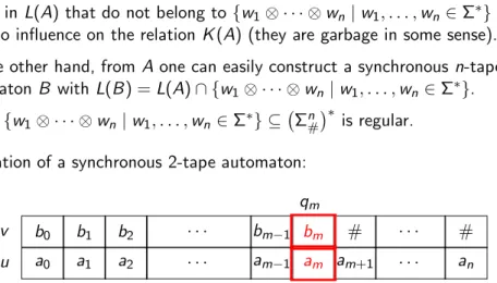
Words in L(A) that do not belong to{w1⊗ · · · ⊗wn|w1, . . . ,wn∈Σ∗} have no influence on the relation K(A) (they are garbage in some sense).
On the other hand, from Aone can easily construct a synchronousn-tape automaton B withL(B) =L(A)∩ {w1⊗ · · · ⊗wn|w1, . . . ,wn∈Σ∗}. Note: {w1⊗ · · · ⊗wn|w1, . . . ,wn ∈Σ∗} ⊆ Σn#∗
is regular.
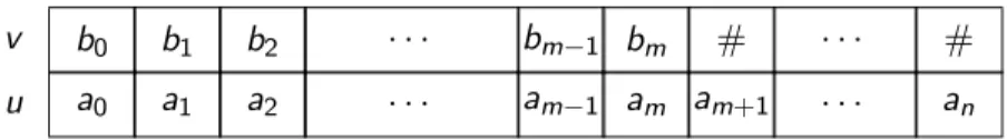
Illustration of a synchronous 2-tape automaton:
u v
a0 b0
a1 b1
a2 b2
· · ·
· · ·
am−1 bm−1
am bm
am+1
#
· · ·
· · · an
#
Synchronous multi-tape automata
Words in L(A) that do not belong to{w1⊗ · · · ⊗wn|w1, . . . ,wn∈Σ∗} have no influence on the relation K(A) (they are garbage in some sense).
On the other hand, from Aone can easily construct a synchronousn-tape automaton B withL(B) =L(A)∩ {w1⊗ · · · ⊗wn|w1, . . . ,wn∈Σ∗}. Note: {w1⊗ · · · ⊗wn|w1, . . . ,wn ∈Σ∗} ⊆ Σn#∗
is regular.
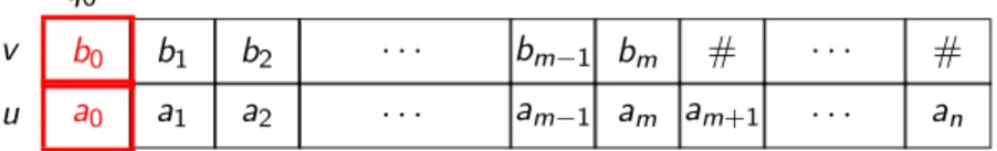
Illustration of a synchronous 2-tape automaton:
q0
u v
a1 b1
a2 b2
· · ·
· · ·
am−1 bm−1
am bm
am+1
#
· · ·
· · · an
# a0
b0
Synchronous multi-tape automata
Words in L(A) that do not belong to{w1⊗ · · · ⊗wn|w1, . . . ,wn∈Σ∗} have no influence on the relation K(A) (they are garbage in some sense).
On the other hand, from Aone can easily construct a synchronousn-tape automaton B withL(B) =L(A)∩ {w1⊗ · · · ⊗wn|w1, . . . ,wn∈Σ∗}. Note: {w1⊗ · · · ⊗wn|w1, . . . ,wn ∈Σ∗} ⊆ Σn#∗
is regular.
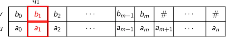
Illustration of a synchronous 2-tape automaton:
q1
u v
a0 b0
a2 b2
· · ·
· · ·
am−1 bm−1
am bm
am+1
#
· · ·
· · · an
# a1
b1
Synchronous multi-tape automata
Words in L(A) that do not belong to{w1⊗ · · · ⊗wn|w1, . . . ,wn∈Σ∗} have no influence on the relation K(A) (they are garbage in some sense).
On the other hand, from Aone can easily construct a synchronousn-tape automaton B withL(B) =L(A)∩ {w1⊗ · · · ⊗wn|w1, . . . ,wn∈Σ∗}. Note: {w1⊗ · · · ⊗wn|w1, . . . ,wn ∈Σ∗} ⊆ Σn#∗
is regular.
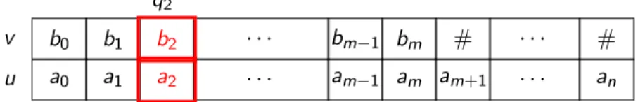
Illustration of a synchronous 2-tape automaton:
q2
u v
a0 b0
a1 b1
· · ·
· · ·
am−1 bm−1
am bm
am+1
#
· · ·
· · · an
# a2
b2
Synchronous multi-tape automata
Words in L(A) that do not belong to{w1⊗ · · · ⊗wn|w1, . . . ,wn∈Σ∗} have no influence on the relation K(A) (they are garbage in some sense).
On the other hand, from Aone can easily construct a synchronousn-tape automaton B withL(B) =L(A)∩ {w1⊗ · · · ⊗wn|w1, . . . ,wn∈Σ∗}. Note: {w1⊗ · · · ⊗wn|w1, . . . ,wn ∈Σ∗} ⊆ Σn#∗
is regular.
Illustration of a synchronous 2-tape automaton:
qm
u v
a0 b0
a1 b1
a2 b2
· · ·
· · ·
am−1 bm−1
am+1
#
· · ·
· · · an
# am
bm
Synchronous multi-tape automata
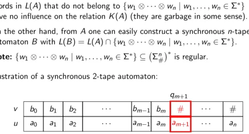
Words in L(A) that do not belong to{w1⊗ · · · ⊗wn|w1, . . . ,wn∈Σ∗} have no influence on the relation K(A) (they are garbage in some sense).
On the other hand, from Aone can easily construct a synchronousn-tape automaton B withL(B) =L(A)∩ {w1⊗ · · · ⊗wn|w1, . . . ,wn∈Σ∗}. Note: {w1⊗ · · · ⊗wn|w1, . . . ,wn ∈Σ∗} ⊆ Σn#∗
is regular.
Illustration of a synchronous 2-tape automaton:
qm+1
u v
a0 b0
a1 b1
a2 b2
· · ·
· · ·
am−1 bm−1
am bm
· · ·
· · · an
# am+1
#
Synchronous multi-tape automata
Words in L(A) that do not belong to{w1⊗ · · · ⊗wn|w1, . . . ,wn∈Σ∗} have no influence on the relation K(A) (they are garbage in some sense).
On the other hand, from Aone can easily construct a synchronousn-tape automaton B withL(B) =L(A)∩ {w1⊗ · · · ⊗wn|w1, . . . ,wn∈Σ∗}. Note: {w1⊗ · · · ⊗wn|w1, . . . ,wn ∈Σ∗} ⊆ Σn#∗
is regular.
Illustration of a synchronous 2-tape automaton:
qn
u v
a0 b0
a1 b1
a2 b2
· · ·
· · ·
am−1 bm−1
am bm
am+1
#
· · ·
· · · an
#
Synchronous multi-tape automata
Example: Let Abe the following synchronous 2-tape automaton:
p (#,a),(#,b) q
(a,a),(b,b) (#,a),(#,b)
We have K(A) ={(u,v)|u,v ∈ {a,b}∗,∃w ∈ {a,b}∗ :v =uw} (the prefix relation).
On the other hand, the suffix relation {(u,v)| ∃w ∈ {a,b}∗ :v =wu} is not synchronously rational.
Automatic structures
Definition
A relational structure A= (A,R1, . . . ,Rm) (withRi an ni-ary relation) is automatic if there exist a finite alphabet Σ, a finite automatonB over the alphabet Σ, and synchronous ni-tape automataBi over the alphabet Σ (1≤i ≤m) such that:
◮ L(B) =A
◮ K(Bi) =Ri for 1≤i ≤m Definition
A structure Ais automatically presentable ifA is isomorph to an automatic structure.
Automatic structures
Excursion: isomorphic structures
Let A= (A,R1, . . . ,Rm) andB= (B,P1, . . . ,Pm) be relational structures, where Ri andPi are bothni-ary (for all 1≤i ≤m).
We say thatA andB areisomorphic if there is a bijectionh:A→B such that for all 1≤i ≤m and all tuples (a1, . . . ,ani)∈Ani we have:
(a1, . . . ,ani)∈Ri ⇐⇒ (h(a1), . . . ,h(ani))∈Pi.
Intuitively: Bcan be obtained from A by renaming the elements from the universe of A.
If A andB are isomorph then Th(A) is decidable if and only if Th(B) is decidable (predicate logic cannot refer to the names of elements in the universe).
( N, +) is automatic
Theorem
(N,+) with + ={(a,b,c)|a+b =c} is automatically presentable.
Proof:Let Abe a finite automaton with L(A) ={0} ∪ {0,1}∗1.
Then, the following function h:L(A)→Nis a bijection:
h(0) = 0
h(a0a1· · ·an−11) = Xn−1
i=0
ai2i+ 2n
Let B+ be the synchronous 3-tape automaton from the next slide.
B+ “almost” recognizes the relation
{(u,v,w)∈L(A)3 |h(u) +h(v) =h(w)}. We have for instance (00,0000,0000)∈K(B+).
( N, +) is automatic
q1
q0
q2
q4
q3
q5
qf
(#,1,1) (#,0,0)
(0,#,0) (1,#,1) (#,0,0),(#,1,1)
(1,0,1) (0,0,0) (0,1,1)
(0,#,0),(1,#,1) (1,1,0)
(0,0,1) (#,0,1)
(0,#,1) (#,0,1)
(0,#,1)
(#,1,0)
(1,#,0) (#,1,0)
(1,#,0) (1,0,0)
(0,1,0) (1,1,1)
(#,#,1) (#,#,1)
(#,#,1)
( N, +) is automatic
Let A+ be a synchronous 3-tape automaton with
L(A+) =L(B+)∩ {u⊗v⊗w |u,v,w ∈L(A)}. We then get K(A+) ={(u,v,w)∈L(A)3 |h(u) +h(v) =h(w)}. Intuition:The automaton from Slide 56 checks with the school method for addition whether the number on tape 3 is the sum of the numbers on tapes 1 and 2.
For this, the automaton stores the current carry in its state.
States q0,q1,q2 correspond to carry 0 whereas statesq3,q4,q5 correspond to carry 1.
( N, +) is automatic
Three states are needed since the numbers on tapes 1 and 2 may have a different bit lengths.
States q1,q4 (q2,q5) are needed for the situation where the number on tape 1 (2) is shorter than the number on tape 2 (1).
State qf is a failure state.
One can slightly extend the theorem on Slide 55: For every p >1 the structure (N,+,|p) with
x |p y ⇐⇒ ∃n,k ∈N:x=pn ∧ y =k·x is automatically presentable.
Linear orders
Our second example for an automatic structure is a linear order.
Recall (from the lecture DMI): a linear order is a structure (A,R), where R is a binary relation with the following properties:
◮ ∀a∈A: (a,a)∈R (R is reflexive)
◮ ∀a,b∈A: (a,b)∈R∧(b,a)∈R→a=b (R is anti-symmetric)
◮ ∀a,b,c ∈A: (a,b)∈R∧(b,c)∈R→(a,c)∈R (R is transitive)
◮ ∀a,b∈A: (a,b)∈R∨(b,a)∈R (R is linear)
Instead of R we denote the binary relation of a linear order always with≤ (possibly with an index).
An element a∈Ais asmallest(resp., largest) elementof the linear order (A,≤) if:∀b∈A:a≤b (resp., ∀b∈A:b ≤a).
Linear orders
Theorem
The linear order (Q,≤) (where≤is the standard order on Q) is automatically presentable.
For the proof we use a famous theorem of Cantor.
It uses another property of linear orders (we writex <y for x ≤y∧x6=y): A linear order (A,≤) isdense if:
∀x∀y(x <y → ∃z(x<z <y)).
Intuitively: between two different elements of Athere is always a third element.
Cantor’s theorem
Let (A,≤A) and (B,≤B) be countable dense linear orders without a smallest and largest element. Then (A,≤A) and (B,≤B) are isomorphic.
Cantor’s theorem
Proof of Cantor’s theorem:
We construct enumerations
a1,a2,a3,a4, . . . andb1,b2,b3,b4, . . . with the following properties:
◮ ai 6=aj andbi 6=bj for i 6=j
◮ A={ai |i ≥1} andB ={bi |i ≥1}
◮ ai <aj if and only if bi <bj for alli,j.
Then, f :A→B withf(ai) =bi is an isomorphism.
Since AandB are countable and infinite, we can enumerate these sets:
A={x1,x2,x3, . . .} andB ={y1,y2,y3, . . .} The following “algorithm” constructs enumerations with the above properties:
Cantor’s theorem
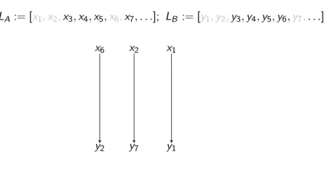
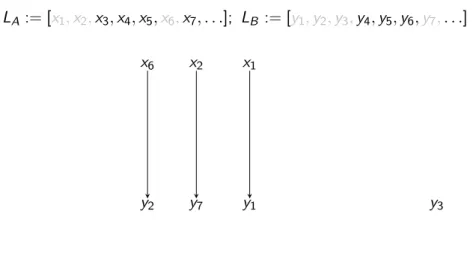
LA := [x1,x2,x3, . . .]; LB := [y1,y2,y3, . . .]
for all i ≥1 do (a1, . . .ai−1,b1, . . .bi−1 are already defined) ifi is odd then
let x be the first element from LA remove x from the list LA
let y be an element fromLB with the following properties:
∀1≤j ≤i−1 :aj <x ←→bj <y (†) remove y from the listLB
ai :=x;bi :=y else
let y be the first element fromLB remove y from the listLB
let x be an element fromLA with the following properties:
∀1≤j ≤i−1 :aj <x ←→bj <y (‡) remove x from the list LA
ai :=x;bi :=y endfor
Cantor’s theorem
Remarks:
◮ The element y with the property (†) exists, since (B,≤B) is dense and neither has a smallest nor largest element.
This ensures that we find forx an elementy that has the same position relative to b1, . . . ,bi−1 asx toa1, . . . ,ai−1.
For the same reason, the element x with the property (‡) exists.
◮ Since the correspondence ai 7→bi must be bijective, we have to pair every element from the listLA with exactly one element from the list LB. Thereby, we also have to ensure that every element from the list LB is paired.
This will be enforced by the case distinction between i odd andi even.
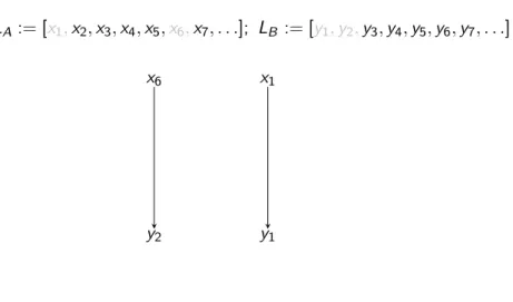
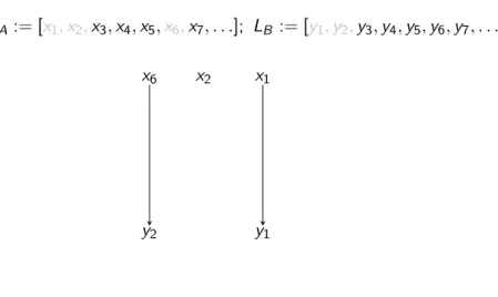
Cantor’s theorem
Illustration of the proof of Cantor’s theorem:
Cantor’s theorem
Illustration of the proof of Cantor’s theorem:
LA := [x1,x2,x3,x4,x5,x6,x7, . . .]; LB := [y1,y2,y3,y4,y5,y6,y7, . . .]