Unclassified ECO/WKP(2006)5

Organisation de Coopération et de Développement Economiques

Organisation for Economic Co-operation and Development

___________________________________________________________________________________________

English - Or. English ECONOMICS DEPARTMENT

PROJECTING OECD HEALTH AND LONG-TERM CARE EXPENDITURES: WHAT ARE THE MAIN DRIVERS?

ECONOMICS DEPARTMENT WORKING PAPERS No. 477

All Economics Department Working Papers are available through OECD's Internet Web site at www.oecd.org/eco

ECO/WKP(2006)5 Un cl assi fi ed Eng lis h - O r. Eng

Cancels & replaces the same document of 03 February 2006

ABSTRACT/RESUMÉ

Projecting OECD health and long-term care expenditures: What are the main drivers?

This paper proposes a comprehensive framework for projecting public heath and long-term care expenditures. Notably, it considers the impact of demographic and non-demographic effects for both health and long-term care. Compared with other studies, the paper extends the demographic drivers by incorporating death-related costs and the health status of the population. Concerning non-demographic drivers of health care, the projection method accounts for income elasticity and a residual effect of technology and relative prices. For long-term care, the effects of increased labour participation, reducing informal care, and wage inflation are taken into account. Using this integrated approach, public health and long-term care expenditure are projected for all OECD countries for the years 2025 and 2050. Alternative scenarios are simulated, in particular a 'cost-pressure' and 'cost-containment' scenario, together with sensitivity analysis. Depending on the scenarios, the total health and long-term care spending is projected to increase on average across OECD countries in the range of 3.5 to 6 percentage points of GDP for the period 2005-2050.

JEL Classification: H51, I12, J11, J14

Key words: Public health expenditures, long-term care expenditures, ageing populations, longevity, demographic and non-demographic effects, projection methods.

******

Cette étude propose un cadre assez complet pour effectuer des projections de dépenses de soins de santé et de soins de long terme. Notamment, à la fois pour les dépenses de santé et les soins de long terme, les effets des facteurs démographiques et non démographiques sont considérés dans l'analyse. En comparaison avec d'autres études, les effets démographiques ont été élargis pour incorporer les coûts liés à la mortalité et à l'état de santé de la population. Pour ce qui concerne les facteurs non démographiques des dépenses de santé, la méthode de projection incorpore un effet d'élasticité-revenu et l'effet résiduel de la technologie et des prix relatifs. Pour les soins de long terme, l'effet d'une participation accrue dans le marché du travail diminuant l'offre de soins informels, et de l'inflation des salaires ont été pris en compte. Sur la base de cette approche intégrée, les dépenses publiques de santé et des soins de long terme sont projetées pour tous les pays de l'OCDE et pour les années 2025 et 2050. Des scénarios alternatifs ont été simulés, en particulier un

"scénario de pression sur les coûts" et un "scénario de contention des coûts", ainsi qu’une analyse de sensitivité. En fonction des scénarios, le total des dépenses de santé et des soins de long terme est projeté d'augmenter pour la moyenne de l’OCDE entre 3.5 et 6 points de PIB pour la période 2005-2050.

Classification JEL: H51, I12, J11, J14

Mots clefs: dépenses publiques de santé, dépenses publiques de soins à long terme, vieillissement de la population, longévité, effets démographiques et non démographiques, méthodes de projection.

Copyright OECD, 2006

Applications for permission to reproduce or translate all, or part of, this material should be made to:

Head of Publications Service, OECD, 2 rue André-Pascal, 75775 Paris Cedex 16, France.

TABLE OF CONTENTS

FOREWORD ... 5

1. Summary and main findings... 6

2. Health care... 10

Projecting demographic drivers of expenditure... 10

Projecting non-demographic drivers of expenditure... 12

Combining demographic and non-demographic drivers... 14

Alternative scenarios for OECD countries ... 15

Demographic effects ... 15

A cost pressure scenario... 16

A cost-containment scenario ... 16

Sensitivity analysis ... 17

Residuals, income elasticity and different health scenarios... 17

Alternative population projections... 18

3. Long-term care ... 18

Projecting demographic drivers of expenditure... 19

Projecting non-demographic drivers of expenditure... 20

Combining demographic and non-demographic drivers... 21

Alternative scenarios for OECD countries ... 22

Demographic effects ... 22

A cost-pressure scenario ... 23

A cost-containment scenario ... 23

Sensitivity analysis ... 23

REFERENCES ... 25

ANNEX 1. LIST OF TABLES AND FIGURES... 30

ANNEX 2A. DATA SOURCES AND METHODS... 50

Macro data ... 50

Health care... 50

Estimating the death-related costs... 50

Estimating the survivors' expenditure curves... 51

Calibration of the cost curves on the OECD Health database... 51

Projecting the demographic effects under a ‘healthy ageing’ scenario... 51

Long-term care (LTC) ... 52

Expenditure curves... 52

The starting point of the projections ... 53

Detailed results for the projection scenarios... 53

ANNEX 2B. EMPIRICAL EVIDENCE ON THE HEALTH CARE INCOME ELASTICITIES ... 73

A brief survey of the literature... 73

Econometric estimates ... 74

ANNEX 2C. OBESITY TRENDS IN OECD COUNTRIES ... 77

Boxes

Box 1. Glossary of technical terms ... 9

Box 2. Longevity and health status scenarios ... 11

Box 3. Cost-containment policies in OECD countries: an overview ¹ ... 13

Box 4. Exogenous variables and assumptions underlying the projections... 15

Box 5. Has disability fallen over time? ... 20

FOREWORD

Rising expenditure on health and long-term care is putting pressure on government budgets in most OECD countries. Going forward, these pressures will add to those arising from insufficiently reformed retirement schemes. The question is how much health and long-term care spending could increase in the future and what policy can do about it. This paper presents a framework for thinking about that question and provides some quantitative illustrations. Both changing demography and non-demographic drivers of spending are taken into account.

The paper shows that spending on health and long-term care is a first-order policy issue. Between now and 2050, public spending on health and long-term care could almost double as a share of GDP in the average OECD country in the absence of policy action to break with past trends in this area. And that estimate takes into account that as people live longer, they also remain in good health for longer. Even with containment measures, public spending on health and long-term care could rise from the current average level of 6-7 % of GDP to around 10% by 2050. In some countries, the increase could be dramatic.

Despite the orders of magnitudes involved, policy discussion in many countries has focused less on health and long-term care spending than on pension and transfer spending. There can be many reasons for that.

One is possibly that pension spending is analytically more easily tractable than is the case for health and long-term care. Another is that the policy instruments to address pension spending are more readily identifiable. A third is that it is easier in the case of pensions to identify benchmarks for assessing what constitutes reasonable spending levels and sensible incentives to private sector actors. Whatever the reasons, the results in this paper illustrate that the policy environment for health and long-term care spending is of primordial importance.

The work behind this report was undertaken by a team led by Joaquim Oliveira Martins and comprising also Christine de la Maisonneuve and Simen Bjørnerud. As usual in our work, a preliminary version of the report was discussed by OECD government representatives. They provided many helpful comments, but the responsibility for the final product of course lies with the OECD Secretariat.

Jean-Philippe Cotis

Chief Economist

PROJECTING OECD HEALTH AND LONG-TERM CARE EXPENDITURES: WHAT ARE THE MAIN DRIVERS?

1. Summary and main findings

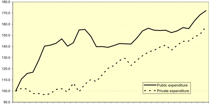
1. Public spending on health and long-term care is a major source of fiscal pressures in most OECD countries, amounting to, on average, some 7% of GDP in 2005. Evolution has been uneven over time:

following rapid growth during the 1970s, public spending slowed down for several decades. However, a recent acceleration (Figure 1.1) has raised concern about likely future trends.

[Figure 1.1 Evolution of public and private OECD health spending]

2. This paper attempts to respond to these concerns by considering a number of factors likely to drive public spending on health and long-term care over the period to 2050. ¹ In projecting drivers of this spending, two important distinctions are made:

• Expenditures on long-term care and on health care (both preventive and acute) are examined separately,

• For both health and long-term care, the impacts of ageing and non-demographic factors are brought separately into the analysis.

3. The projections rely on a uniform cross-country framework, in contrast with an earlier OECD exercise. ² The latter essentially gathered country-specific projections, provided by national authorities, produced on the basis of an agreed set of macroeconomic and demographic assumptions. The current projections are more homogeneous, but at the cost of simplifying the description of national health and long-term care arrangements. The main purpose is to bring out in a stylised and tractable way the key mechanisms at work. The inherent uncertainties surrounding this approach are addressed by analysing the sensitivity of the projection results to changes in the assumptions concerning the main drivers of expenditure.

4. In broad terms, the principal forces driving these projections are (see main text for detail):

• Health care, demographic factors: a rising share of older age groups in the population will put upward pressure on costs because health costs rise with age. However, the average cost per individual in older age groups should fall over time for two reasons:

− Longevity gains are assumed to translate into additional years of good health (“healthy ageing); and

1. This paper only deals with public spending. Private spending added another 2% of GDP on average to expenditure on health and long-term care in 2005. While it could be argued that private and public expenditures are not separable, it is implicitly assumed here that private health spending arises from individual choices and, therefore, could be treated like any other consumption item.

2. For details on this earlier project see Dang et al. (2001).

− Major health costs come at the end of life. Insofar as increasing longevity means that more individuals “exit” an age group by living into an older group (rather than “exit” by dying), average costs of the group in question will fall.

• Health care, non-demographic factors: health care costs have typically grown faster than income (even as incomes have increased). This is generally held to be due to the effect of technology and relative-price movements in the supply of health services. Disentangling these factors is beyond the scope of current analysis and indeed is dealt with only modestly in the literature. Hence, two scenarios are assumed in the projections here:

− A “cost pressures” scenario in which it is assumed that, for given demography, expenditures grow 1% per annum faster than income. This corresponds to observed trends over the past two decades.

− A “cost-containment” scenario in which (unspecified) policy action is assumed to curb this

“extra” expenditure growth such that it is eliminated by the end of the projection period (2050).

• Long-term care, demographic factors: dependency on long-term care will tend to rise as the share of old people in the population increase. This effect is mitigated somewhat by the likelihood that the share of dependents per older age group will fall as longevity increases due to

“healthy ageing”.

• Long-term care, non demographic factors: expenditures are likely to be pushed up by a possible

“cost disease” effect, i.e. the relative price of long-term care increasing in line with average productivity growth in the economy because the scope for productivity gains in long-term care is more limited. ³ This effect is assumed to be fully operative in the “cost pressure” scenario but to be partially mitigated ⁴ by (unspecified) policy action in the “cost containment” scenario.

5. As noted, two main sets of scenarios were simulated, one in which no policy action is assumed, the “cost pressures” scenario, and a “cost-containment scenario” that embodies the assumed effects of policies curbing expenditure growth. As mentioned above, these policies are not modelled explicitly.

Finally, sensitivity tests were carried out to assess the robustness of the results to key assumptions.

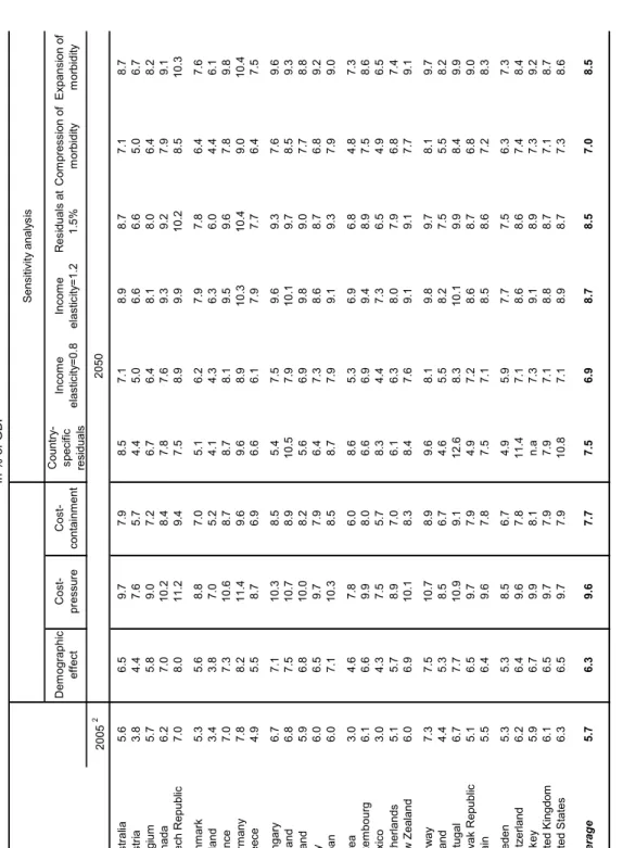
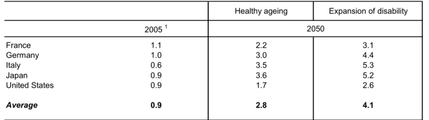
6. The projections for health and long-term care expenditures yield the following stylised results (Table 1.1):

• In the “cost-pressure” scenario average health and long-term care spending across OECD countries is projected to almost double from close to 7% of GDP in 2005 to some 13% by 2050.

• In the “cost-containment” scenario, average expenditures would still reach around 10% of GDP by 2050, ⁵ or an increase of 3½ percentage points of GDP.

3. Note that empirical evidence on the income elasticity of long-term care spending simply does not exist, and in most scenarios it is assumed to be zero.

4. It is arbitrarily assumed that the relative price changes by only half of productivity growth elsewhere in the economy.

5. As a comparison, on the basis of pure demographic effects, Dang et al. (2001) concluded that the

expenditure on health and long-term care for a group of OECD countries would increase from 6% of GDP

in 2000 to 9 to 9½ per cent of GDP in 2050. A similar study by the EC-Economic Policy

• Non-demographic factors (including effects from technology and relative prices) play a significant role in upwards pressure on long-term care expenditures, and indeed are the most important driver of the increase in health-care expenditure.

[Table 1.1 Public health and long-term care spending]

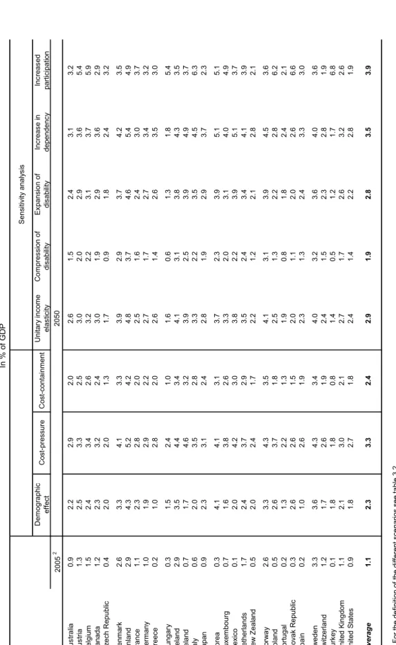
7. These average results hide striking differences across countries (Figure 1.2). In the cost- containment scenario, a group of countries stands out with increases of health and long-term care spending at or above four percentage points of GDP, over the period 2005-50. It includes rapidly ageing countries (Italy, Japan, Spain), countries that will experience a dramatic change in their population structure (Korea, Mexico, Slovak Republic), and countries with currently low labour participation, which may face a substantial increase in the demand for formal long-term care (Italy, Ireland, Spain). In contrast, Sweden is in the lowest range with an increase below two percentage points of GDP. This country is in a mature phase of its ageing process and already spends a relatively high share of GDP on health and long-term care.

[Figure 1.2 Total increase in health and long-term care spending, 2005-2050]

8. Despite the uncertainties, sensitivity analysis suggests the results are fairly robust in key respects.

For example, under the assumption of “healthy ageing” changes in longevity will have only a modest effect on spending. However, the projections for spending on long-term care are sensitive to the future development of participation rates for the working-age population because higher participation reduces the capacity for “informal” care. An alternative scenario, where participation rates in countries where they are currently low converge towards levels in high-participation countries, has spending on long-term care rising by an additional 1-2% of GDP on average, but much more in some countries. ⁶

9. The paper follows the structure displayed in Figure 1.3. It begins with health care expenditure, decomposing demographic and non-demographic expenditure drivers, discusses the main mechanisms at work in each case, and describes the projection framework. Alternative projection scenarios are then presented, followed by a discussion of the sensitivity of the results to key assumptions. The same sequence applies to long-term care expenditures. A glossary of technical terms is provided in Box 1.

[Figure 1.3 Drivers of total health and long-term care spending: key components]

Committee (2001), focusing on the EU15 area, calculated that the expenditure on health and long-term care would increase from 6½ per cent in 2000 to 8½ to 9% in 2050. Calculated in the same way, the ageing effect was estimated to be of comparable size also in Canada (Health Canada, 2001). These orders of magnitude are comparable with the results of the present study, but the underlying drivers are rather different. For an update of the assumptions and projection methodologies see EC-Economic Policy Committee (2005).

6. However, higher participation rates are likely to have positive effects on public budgets which, depending

on how they come about, may more than offset the effect via long-term care spending.

Box 1. Glossary of technical terms

Activities of daily living (ADLs) Self-care activities that a person must perform every day, such as bathing, dressing, eating, getting in and out of bed, moving around, using the toilet, and controlling bladder and bowel.

(Acute) health care Is distinguished from long-term care in the sense that acute health care aims at changing the medical condition of a person (e.g. surgery) while long-term care only compensates for lasting ability.

Baumol effect or 'cost-disease' Tendency for relative prices of some services, such as long-term care, to increase vis-à-vis other goods and services in the economy, reflecting a negative productivity differential and the equalisation of wages across sectors.

Compression of morbidity The hypothesis that increases in longevity translate into a shorter share of life lived in relatively bad health.

Death-related costs Health expenditures incurring at the end of life. One hypothesis proclaims that the apparent rise in health expenditures with age reflects the fact that death is more frequent at higher ages, not merely the fact that people are old and frail. Following this line of thought, the projected fall in mortality will damp the future impact of ageing.

Disability/dependency Inability to perform one or more ADLs without help. Specific definitions, i.e. how many ADLs, differ across countries making comparisons difficult.

Dynamic equilibrium (“healthy ageing”) The hypothesis that the number of years of life lived in bad health remains constant in the wake of increased longevity (or increased life expectancy is translated into additional years in good health).

Expansion of morbidity The hypothesis that increases in longevity translate into a higher share of life lived in relatively bad health.

Formal long-term care Long-term care services supplied by the employees of any organisation, in either the public or private sector, including care provided in institutions like nursing homes, as well as care provided to persons living at home by either professionally trained care assistants, such as nurses, or untrained care assistants. Divided into home care and institutional care.

Informal care Long-term care provided by spouses/partners, other members of the household and other relatives, friends and neighbours. Informal care is usually provided at the home and is typically unpaid.

Long-term care A range of (often basic) services needed for persons who are dependent on help for carrying out basic ADLs. Divided into formal and informal long-term care where, on average across OECD countries, the latter currently makes up the bigger part.

Morbidity/chronic conditions A wider concept than disability. Higher levels of disability are generally accompanied by more chronic conditions, but the opposite does not necessarily follow; intensive medical treatment can reduce disability by soothing chronic diseases. This implies that a decline in disability does not necessarily means curtailment in costs. Still, analyses usually focus on disability due to lack of reliable and objective measures of morbidity.

Prevalence of disability/morbidity/

dependency

Number of cases of disability/disease/dependency for a given population for a given

time period. Prevalence of disability/morbidity/dependency tends to be more frequent

at higher ages.

2. Health care

10. Looking at the recent past, expenditures on health care have increased in terms of their share in GDP. Given that pure demographic factors have so far been weak, this upward trend in spending is probably due to the increased diffusion of technology and relative price changes. Two important questions are then: how will these typically non-demographic drivers behave in the future and will the projected change in demographic trends create additional expenditure pressures?

Projecting demographic drivers of expenditure

11. While the effect of ageing on public health expenditures per capita has been weak in the past, ⁷ it is commonly expected that it will increase in the future. This assessment is based on the combined effect of the projected increase in the share of old people and the tendency for health expenditures per capita to increase with age. ⁸

12. In this study expenditure profiles are a central piece of the projection framework (Figure 2.1).

Average health expenditures by age group are relatively high for young children; they decrease and remain stable for most of the prime-age period, and then start to increase rapidly at older ages. ⁹

[Figure 2.1 Public health care expenditure by age groups]

13. For any given year, the population can be divided into two segments: the survivors and the non- survivors. Each of these segments of the population has a specific cost curve. The non-survivors' cost curve can be estimated by multiplying the estimated costs of death by age group by the number of deaths per age group. In line with evidence that health costs are concentrated in the proximity to death (i.e., they are

“death-related”; Seshamani and Gray, 2004; Batljan and Lagergren, 2004), the cost of death was proxied by the health expenditure per capita for the oldest age group (95+) multiplied by a factor (equal to 4 for an individual between 0 to 59 years old and declining linearly to 1 afterwards). The survivors' cost curve can then be derived from the difference between the total cost curve and the non-survivor curve (see Annex 2A). An example of this split is given for one country, Finland, in Figure 2.2. Using this framework, health expenditures for survivors and non-survivors can be projected separately in a more meaningful way.

[Figure 2.2 Breakdown of the health care cost curve]

7. See Culyer (1990), Gerdtham et al., (1992), Hitiris and Posnett (1992), Zewifel et al. (1999), Richardson and Roberston (1999), Moise and Jacobzone (2003) and Jönsson and Eckerlund (2003).

8. Across all health expenditure types, expenditure on those aged over 65 is around four times higher than on those under 65. The ratio rises to between six to nine times higher for the older groups (Productivity Commission, 2005; OECD Health Database, 2005).

9. The data is based on the EU-AGIR Project; see Westerhout and Pellikaan (2005). The complete expenditure profiles were only available for a subset of OECD countries. A number of different adjustments and estimations were made in order to derive these curves for other OECD countries.

Moreover, for some countries only total costs were available and thus health care had to be separated from

long-term care. For 12 countries, the data were simply not available. In this case, the expenditure curves

were estimated by adjusting expenditures as a spline function of age, based on available data, and were

calibrated on the basis of total health expenditures derived from OECD (2005a). These estimation

procedures are described in detail in Annex 2A.

14. The shape of the aggregate cost curves can be explained by movements across age groups in health care expenditures for these two segments of the population. Indeed, the upward shape of the average cost curve reflects the fact that mortality rates are higher for older age groups. At the same time, the fact that the cost curves tend to peak and then decline at very old ages can be explained by considerations related to the cost of death. While the probability of dying increases with age, the costs of death tend to decline steadily after young and prime ages (Aprile, 2004). Finally, the little spike in health expenditures at the youngest age is related in part to infant mortality being higher than prime-age mortality.

15. Noteworthy, the death-related costs hypothesis has logical implications for the health status of survivors. In the extreme case where health costs are only death-related, there are only two outcomes: an individual either dies or survives in good health. To be consistent over time the projected increase in life expectancy must be accompanied by an equivalent gain in the numbers of years spent in good health.

Otherwise, an increasing share of the population living in “bad health” would emerge. Average health care costs would then cease to be mainly driven by the costs of death, as initially assumed.

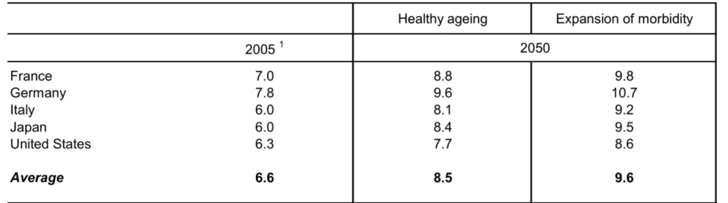
16. Thus, the death-related costs hypothesis implies that longevity gains are translated into years in good health. Under this “healthy ageing” scenario, the cost curve for survivors is allowed to shift rightwards, progressively postponing the age-related increases in expenditure. ¹⁰ This development tends to reduce costs compared with a situation in which life expectancy would not increase. Other health status scenarios have been envisaged in previous research (see Box 2) and the projections in this paper test the sensitivity of the results to these alternative assumptions.

17. As regards non-survivors, two different demographic effects are at play. On the one hand, the number of deaths is set to rise due to the transitory effect of the post-war baby-boom. On the other hand, if mortality falls over time, due to a permanent increase in longevity, fewer will be at the very end of life in each given year, mitigating health care costs. ¹¹ The total effect on public health care expenditures will depend on the relative size of these effects.

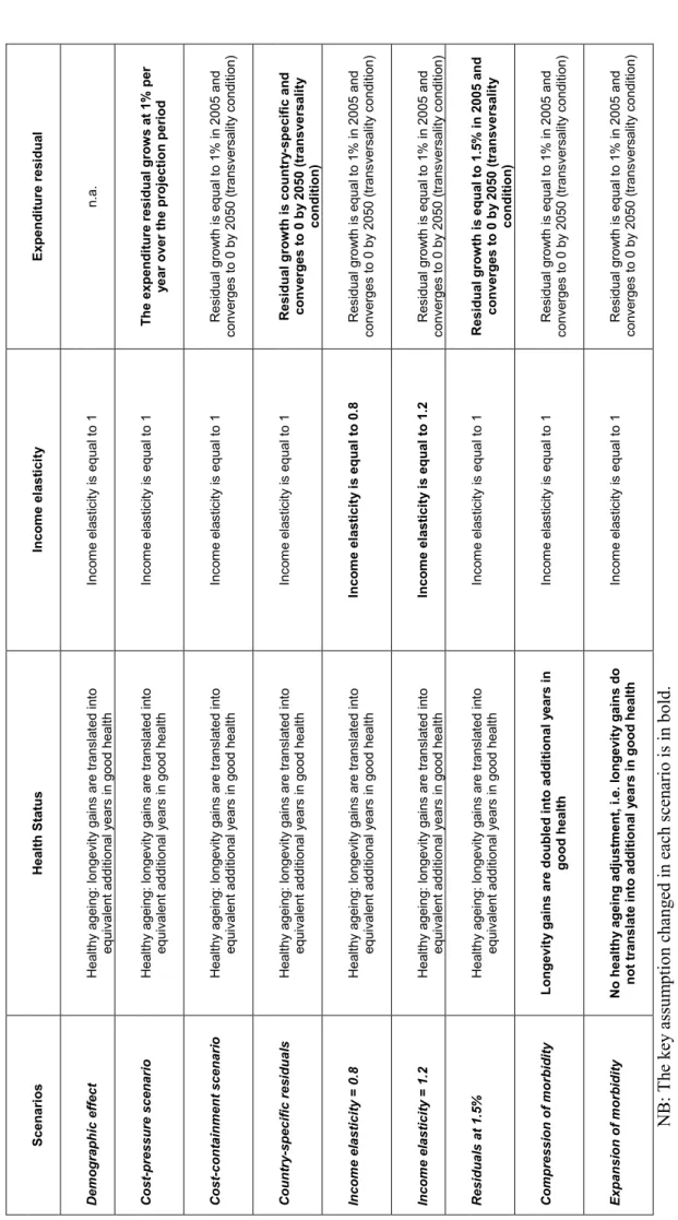
Box 2. Longevity and health status scenarios

Different health status scenarios have been envisaged in the literature. In an “expansion of morbidity” scenario (Grunenberg, 1977), the share of life spent in bad health would increase as life expectancy increases, while a

”compression of morbidity” scenario (Fries, 1980) would mean the opposite. Currently, equilibrium between longevity and morbidity is observed in many OECD countries. Accordingly, and striking a compromise between the expansion and compression scenarios, Manton (1982) put forward the ”dynamic equilibrium” hypothesis where longevity gains are translated one-to-one into years in good health (hereafter, referred as ”healthy ageing”).

In this context, Michel and Robine (2004) proposed a general approach to explain why countries may shift from an expansion to a contraction of morbidity regime, or achieve a balanced equilibrium between longevity gains and the reduction of morbidity. They identified several factors at work: i) an increase in the survival rates of sick persons which would explain the expansion in morbidity; ii) a control of the progression of chronic diseases which would explain a subtle equilibrium between the fall in mortality and the increase in disability; iii) an improvement in the health status and health behaviour of the new cohorts of old people which would explain the compression of morbidity, and eventually; iv) the emergence of very old and frail populations which would explain a new expansion in morbidity.

Depending on the relative size of each of these factors, countries could evolve from one morbidity regime to another.

10. In contrast, in a “pure demographic” approach to health care expenditures, the cost curves would not shift rightwards with ageing, reflecting the implicit assumption of unchanged health status at any given age.

When the cost curves stay put in presence of longevity gains, the share of life lived in ‘bad health’

increases when life expectancy increases.

11. See for example Fuchs (1984), Zwiefel et al. (1999), Jacobzone (2003) and Gray (2004).

Projecting non-demographic drivers of expenditure

18. Income growth is certainly the main non-demographic driver of expenditures, although the vast literature on this topic is still somewhat inconclusive on the precise value of the income elasticity (see Annex 2B). Two insights can, nevertheless, be drawn. First, income elasticity tends to increase with the level of aggregation, implying that health care is both “an individual necessity and a national luxury”

(Getzen, 2000). Second, without reliable price data for health-related goods and services, the high income elasticities (above unity) often found in macro studies may result from the failure to control for true price effects. In this context, the most reasonable approach seems to assume unitary income elasticity and, subsequently, to test the sensitivity of the projections to this assumption.

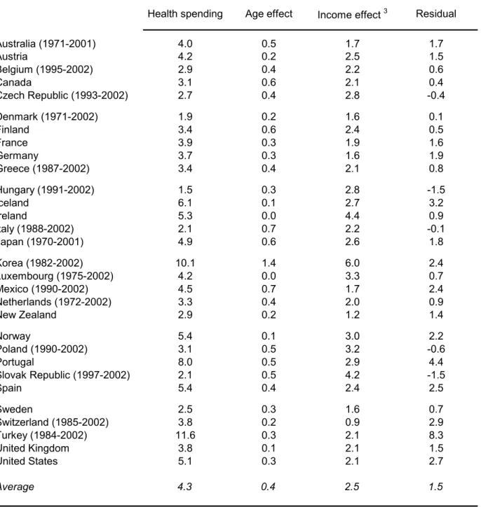
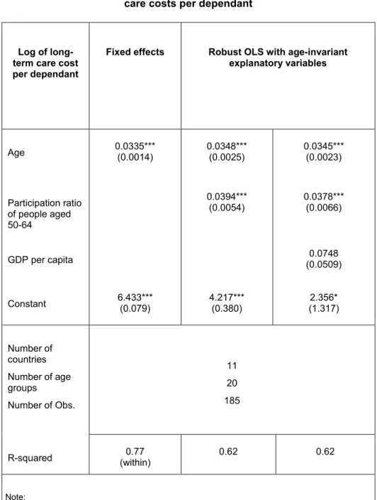
19. After controlling for demographic and income effects, a residual expenditure growth can be derived. Between 1981 and 2002 (Table 2.1), public health spending grew on average by 3.6% per year for OECD countries, ¹² of which 0.3 percentage point was accounted by pure demographic effects ¹³ and 2.3 percentage points by income effects (assuming unitary income elasticity). Thus, the residual growth can be estimated at around 1% per year. Over an extended sample, 1970-2002, the residual growth would much higher to reach 1.5% per annum (Table 2.2). This difference reflects the implementation of cost- containment policies over part of the 1980s and the 1990s that curbed the strong residual growth of the 1970s (Box 3).

[Table 2.1 Decomposing growth in public health spending, 1981-2002]

[Table 2.2 Decomposing growth in public health spending, 1970-2002]

20. What are the factors underlying this residual expenditure growth? The main culprits seem to be technology and relative prices. ¹⁴ Indeed, the gains in health status discussed above do not only arise from improvements in lifestyle (Sheehan, 2002; Cutler, 2001), but also from advances in medical treatment/technology. The latter, however, do not come free of economic cost. Technical progress can be cost-saving and reduce the relative price of health products and services, but its impact on expenditure will depend on the price elasticity of the demand for health care. If it is high, a fall in prices will induce a more than proportionate rise in demand, increasing expenditures. ¹⁵ Even if prices do not fall, new technologies may increase demand by increasing the variety and quality of products. ^16,17

12. This estimate was carried out for total health spending given that the split between health care and long- term care expenditures is not available in time series for historical data. Given the low share of public long- term care expenditure to GDP in 2000 (typically below 1% of GDP; OECD, 2005b), this approximation of the residual growth seems reasonable.

13. To simplify calculations, the effect of past ageing does not incorporate “healthy longevity” and “death- related cost” as is done in the projections. In any event, the ageing effect was small and would have even been even smaller if a more sophisticated method had been applied. If anything, ceteris paribus, ignoring these past factors is likely to have lead to a downward bias in the estimated residual.

14. See Fuchs (1972) and Mushkin and Landefeld (1979). More recently, there has been a renewal of interest in this approach, see Newhouse (1992), KPMG Consulting (2001), Wanless (2001), Productivity Commission (2005a-b).

15. For example, Dormont and Huber (2005) found that in France the unit price of certain surgical treatments, such as cataract, decreased whereas the frequency of the treatments increased significantly. Such effects can explain much of the recent upward shift in the health care cost curves in France.

16. This is equivalent to say that the “true” relative price of health care vis-à-vis all other goods in the economy decreases. Consider for example the case of a demand for variety model with a CES utility function:

∑

=

i

x

U

, where σ>1 is the elasticity of substitution among products.

21. In projecting public health care expenditures, two alternative scenarios were envisaged for the future: one in which the residual effect of technology and prices continues to rise at the historical rate and another in which this rate declines over time due to cost containment policies. Should the country-specific historical growth rates in the residual be used to project expenditures? There are least two reasons for questioning this choice. First, in countries where cost-containment policies have resulted in a low or negative residual (e.g., Austria, Denmark, Ireland, Italy, Sweden) there could be a trend reversal, e.g.

because new personnel has to be attracted or run-down facilities renewed. Second, in countries where the residual growth was very high (e.g., Portugal, Turkey, United States) it may seem likely that cost- containment policies will be implemented in the future. These effects would lead to a certain cross-country convergence of the expenditure residual over time. Therefore, in most of the projection scenarios, an OECD average residual was preferred to project expenditures.

Box 3. Cost-containment policies in OECD countries: an overview

Faced with unsustainable growth in health care spending over the 1960s and 1970s, governments initially aimed at containing it through various kinds of macroeconomic restrictions. These policies often created allocative problems of their own. Wage and price controls had negative consequences on the supply of health while top-down spending constraints also discouraged providers to increase output or to enhance productivity.

More recently the focus turned to more efficient provision of care. Nonetheless, while spending growth has slowed considerably over the past two decades, studies using statistical tests of the impact of budgetary caps or other policies to limit spending provide little evidence of a strong impact. In some cases, the reduction of health care costs has been achieved by transferring spending to other areas, such as long-term care. Supporting this view is the fact that countries that have been most effective at controlling health care spending are also the ones where long-term care expenditures have increased most rapidly.

Macroeconomic cost-containment initiatives

Wage controls have been used in public integrated systems in both the hospital and the ambulatory sector where health care personnel are paid on a salary basis (Denmark (hospitals), Finland, Ireland (hospitals), Spain, Sweden and the United Kingdom (hospitals)). Such policies were part of a broader public sector restraint rather than specific to the health sector.

Price controls have been widely used, particularly in areas where governments set prices administratively or have oversight on prices agreed between health care purchasers and providers. A number of countries have set fees directly (e.g., Australia, Belgium, France, Japan, Luxembourg and Canada). In others, prices have been automatically adjusted to offset volume overrun so as not to exceed a fixed budget ceiling (e.g., Germany (ambulatory care), Austria (hospital care), Hungary (outpatient care), and recent Belgium reforms). Administrative price setting has probably been most widespread for pharmaceutical drugs.

Limits in most countries on entry to medical schools are an important factor affecting the growth of the number of medical professionals. The number of new doctors per capita has slowed as a result. There have also been reductions in support staff (Canada, Sweden). Policies to restrain supply have actually led to supply shortages in, for example, Canada, the United Kingdom and Denmark and waiting lists are a common feature across OECD countries. In countries like Finland, France and Korea an upward pressure on wages has unfolded.

Hospital supply policies have encouraged a reduction in the number of beds per capita and concentrated acute care in larger hospital units so as to achieve economies of scale and scope. Nonetheless, the level of acute-care beds per capita remains relatively high in some countries (such as Austria, the Czech Republic, Germany, Hungary and the Slovak Republic).

Budgetary caps or controls have been a widely used instrument for controlling expenditure. In general, policies to control and reshape supply and to cap spending in the hospital sector appear to have been more successful than for ambulatory care or pharmaceutical drugs. Spending control through budgetary caps also appears to have been most successful in countries such as Denmark, Ireland, New Zealand and the United Kingdom where integrated models of health-care financing and supply are (or were)

To simplify, let us assume price symmetry ( p

= p , ∀ i ). The true composite price index is then equal to

p n

P

=

⋅ . With two types of composite goods, say health (H) and all other goods (O), the true relative price would be: P

P

= ( n

n

)

⋅ ( p

p

) . Thus, even if the usual price ratio ( p _H / p _O ) remains constant, the “true” relative price P _H ^* / P _O ^* would decrease when the pace of product creation in the health sector is much faster than in the rest of the economy.

17. Some governments are attempting to introduce such quality adjustments in the measure of output (and

hence prices) of public services. See Grice (2005) for a discussion on this point based on the Atkinson

Review, prepared for the UK Office for National Statistics.

the rule and in mainly single-payer countries, such as Canada, where health-care budgets are generally explicitly set through the budget process.

Cost sharing has been an increasingly common feature over the 1980s and, particularly, the 1990s. Greater cost-sharing has mainly affected pharmaceuticals, while patient payments for inpatient and doctors visits have been less widespread (Sweden, Italy, France). This is presumably connected to the higher price elasticity for pharmaceutical drugs than for ambulatory and, particularly, for hospital care.

Improving cost-efficiency at the micro level

Ambulatory care is of key importance to the overall efficiency and effectiveness of health-care systems; it usually is the place where contact between patient and health care personnel is first established and ambulatory care is generally less expensive than hospital care. The gate-keeping role of general practitioners (GPs) has been encouraged in some countries (United Kingdom, New Zealand, Norway, United States and France). In Eastern European countries, the ambulatory sector has been shifted from the public sector to private practitioners in the course of the 1990s and, in some cases, they are now paid on a capitation basis.

Hospital sector reforms concern first and foremost the separation of purchasers and providers within public integrated systems.

Purchasers/funders of health care are responsible to the budgetary authorities for cost control and to patients for the quality and accessibility of care. A significant number of countries with integrated systems have now moved in this direction (Australia, United Kingdom, New Zealand, Sweden, Italy, Portugal and, more recently, Greece). More active purchasing has also occurred in countries with public contract models (Germany, Belgium). The role of purchasers has been enhanced in the United States. The contracting out of selected activities has increased, where these can be provided more cheaply externally. Finally, a limited number of countries (the United States, the United Kingdom, Sweden, the Czech Republic and New Zealand) have experimented with greater competition among hospitals as a means of inducing improvement in efficiency, quality, and responsiveness.

____________

1. This Box is based on and draws extensively on Docteur and Oxley (2003).

Combining demographic and non-demographic drivers

22. To sum up, defining HE, Y and N as real health care expenditures, real income and population, respectively; and, ε the income elasticity of health expenditures, the growth of health expenditures can be decomposed as follows:

( ^residual )

N factor Y

age adjusted N

HE log( ) log log

log  + ∆



 



∆ 

⋅ +

∆

 =



 



∆  ε ⁽¹⁾

or expressed in share of expenditure to GDP:

( ^residual )

N factor Y

age adjusted Y

HE log( ) ( 1 ) log log

log  + ∆



 



∆ 

⋅

− +

∆

 =



 



∆  ε ⁽²⁾

23. The mechanical effect of population ageing on expenditures can be interpreted as first moving up along the cost curve, assuming that the age profile of expenditures remain constant over time (Figure 2.3, Panel 1). This age factor is then adjusted by incorporating the healthy longevity hypothesis, corresponding to a rightward shift of the cost curve (Figure 2.3, Panel 2). ¹⁸ As mentioned above, this shift implies that older people still cost more than the young, but at progressively older ages. Finally, the cost curve may shift upwards (Figure 2.3, Panel 3) due to non-demographic drivers (income and the residual).

[Figure 2.3 Shifts in expenditure profiles, ageing and non-ageing effects]

18. See Annex 2A for more details.

24. Once the total logarithmic growth rates are estimated for each country, the projection framework computes the changes in expenditure shares to GDP considering a common starting point. The latter is computed as the cross-country average share of public health care spending in GDP in 2005, thus can be viewed as a sort of OECD representative country. The changes in expenditure calculated from this common base are then added to the country-specific initial shares to obtain future projected ratios of expenditure to GDP. This method has two advantages. Over the long run, it makes the projections more comparable across countries, as the effects of the different mechanisms at work during the projection period are isolated from the impact of the initial conditions. ¹⁹ Moreover, it allows a certain catch-up across countries in the ratios of public health care expenditures to GDP.

25. Additional exogenous assumptions underlying the projections for both health and long term care are listed in Box 4 (more details are also provided in Annex 2B).

Box 4. Exogenous variables and assumptions underlying the projections The projections require a set of exogenous data, as follows:

(1) Population projections (N). The population projections were gathered by the OECD Directorate on Employment, Labour and Social Affairs, directly from national sources. Given that the underlying assumptions on fertility and life expectancy are not necessarily uniform across countries (see Oliveira Martins et al., 2005 for a discussion), this paper also uses a population maquette (Gonand, 2005) to test the sensitivity of the results to uniform longevity assumptions for a selected group of countries.

(2) Labour force projections (L/N) rely on previous OECD work (Burniaux et al., 2003). These projections are constructed in the basis of a, so-called, cohort approach. They correspond to a baseline scenario, i.e. the impact of current policies is assumed to influence labour participation over the next decades, but no additional assumptions are made concerning future policy changes.

(3) Labour productivity (Y/L) growth is assumed to converge linearly from the initial rate (1995-2003) to 1.75% per year by 2030 in all countries, except former transition countries and Mexico where it converges only by 2050.

Summary statistics on the exogenous assumptions are provided in Annex 2A. The projected GDP per capita is directly derived from the above exogenous variables (Y/N = Y/L x L/N). This simple framework is not supposed to capture in the best way productivity differentials across countries, but to isolate, as far as possible, the effect of ageing and other demographic factors on the projections.

Alternative scenarios for OECD countries

26. The framework described above was used to project expenditures over the period 2005-50. In the main scenarios, the income elasticity is set to one, thus income effects are not creating additional pressures in terms of expenditure shares to GDP. The main assumptions underlying each projection scenario are listed in Table 2.3.

[Table 2.3 Assumptions underlying the alternative projection scenarios: Health care]

Demographic effects

27. As discussed above, demographic effects on public health care expenditures can be decomposed into the health care costs for survivors, the adjustment for “healthy ageing” and the death-related costs, as shown in Panel A of Figure 2.4. The pure ageing effect can be quite large in some countries, but it tends to

19. Without this specification, spending patterns of countries with equivalent expenditure drivers would

diverge in terms of share of expenditure to GDP merely due to different initial expenditure to GDP ratios.

be compensated by a better health status. The death-related costs account only for a small fraction of the increase in expenditures as a share of GDP. In level terms, they increase from around 5% of total health care spending in 2005 to 7% by 2050.

[Figure 2.4 Demographic effects on health care expenditure]

28. The total effect of demographics on health care expenditures displays a wide cross-country dispersion. It ranges from virtually zero in Sweden to 1.6 percentage points of GDP for Korea. This can be related to differences in evolving population structures, as displayed by the changes in old-age dependency ratios (Panel B of Figure 2.4).

29. However, on average, the demographic effect only accounts for a small increase in expenditure, from 5.7% in 2005 to 6.3% by 2050, or 0.6 percentage points of GDP (Table 2.4). Admittedly, the “healthy ageing” assumption may render the simulation of demographic effects relatively optimistic, but this is in line with observed patterns of health status regimes in many OECD countries. For some countries, such as Australia, the healthy ageing hypothesis may seem less plausible in view of past trends and, therefore, the sensitivity of the results to this assumption was tested below.

[Table 2.4 Projection scenarios for public health care expenditure]

A cost pressure scenario

30. In this scenario it is assumed that, on top of the demographic effects and income effects, the expenditure residual continues to grow at 1% per year over the projection period. This induces a substantial increase in the health expenditures, averaging nearly 4 percentage points of GDP from 2005-2050. In most countries, health care expenditures would then approach or exceed 10% of GDP by the end of the projection period.

31. While these figures may be useful as a benchmark, they do not seem very plausible. It is unlikely that public health care expenditures to GDP could continue to grow at such constant rate, without limit. A long-run convergence (or transversality) condition is therefore considered in the next scenario.

A cost-containment scenario

32. In the “cost-containment” scenario it is assumed that residual expenditure growth converges to zero by 2050, ²⁰ implicitly meaning that policies are effective in controlling expenditure growth driven by some of the non-demographic factors. These policies have been already enacted in the past (see Box 3 above) and could progressively rein in the expenditure residual, for example by ensuring that future technology improvements are mainly used in a cost-saving way. In the absence of additional ageing effects, this would imply that public health care expenditure and income would evolve in parallel over the very long-run. ²¹

20. This is roughly equivalent to assuming that the residual grows at a constant rate of ½ per cent per year.

21. This convergence assumption (or transversality condition) may appear controversial in view of past

experience. The assumption is justified by the fact that the expenditure growth has to be financed by the

public purse. Under perfect health market conditions, a continuing increase in the share of income going to

health care spending could reflect individual preferences. But the health care market is not perfect and

governments are footing most of the bill. Thus, rapid growth of the share of health care spending in income

would have to be compensated by reductions in other public spending items, which may be difficult to

achieve, and/or increased health care charges for individuals. Such cost sharing has already been

introduced in most countries. Similar transversality conditions have also been imposed in other projection

33. Under this rather optimistic scenario, public health care expenditures in the OECD area would still increase on average by two percentage points between 2005 and 2050, from 5.6% to 7.7% of GDP (Table 2.4). Large increases (above 2.5 percentage points of GDP) by 2050 are found (in descending order) in Korea, Slovak Republic, Mexico and Japan. Most of these countries are experiencing a rapid demographic change induced by the sharp fall in fertility rates.

Sensitivity analysis

34. In the sensitivity analysis, a number of parameters were changed compared with the "cost- containment scenario": the size of the income elasticity, the magnitude of the residual, as well as factors underlying health status scenarios and demographic projections. Overall, the previous results seem relatively robust, as these alternative simulations do not change qualitatively the picture emerging from the comparison of the "cost-pressure" and "cost-containment" scenarios discussed above.

Residuals, income elasticity and different health scenarios

35. Unsurprisingly, applying country-specific growth rates of the residual component ²² would significantly affect spending patterns of individual OECD countries (Table 2.4). Korea, Mexico, Portugal, Switzerland, the United States would record significant increases (above two percentage points of GDP) compared with the "cost-containment" scenario. ²³ If anything, this scenario illustrates the unsustainability of current health expenditure trends in some OECD countries. In contrast, in countries where recent cost- containment policies were successful, the projected expenditure shares would tend to be more moderate than in the cost-containment scenario (e.g., Denmark, Sweden). Other countries would display large decreases in expenditures because the effect of past residual growth resulting from idiosyncratic conditions, such as the scaling back of former welfare systems during economic transition (Czech Republic, Hungary, Poland and Slovak Republic), would be prolonged in the future.

36. To assess sensitivity to income elasticity, projections were run with elasticities below and above unity (0.8 and 1.2, respectively), while keeping the residual as in the cost-containment scenario. ²⁴ Under these alternative scenarios, average OECD public health care expenditure shares would range from around 7% to 8.7% of GDP. The countries with the largest projected GDP per capita growth (e.g. Ireland, Mexico, Poland, see Table A2.1 in Annex 2A) are obviously the most affected by changes in income elasticity.

37. As discussed above, the residual was derived from trends observed over the two past decades, a period characterised by efforts to contain costs. Assuming that the residual would grow at 1.5% per year (as observed on average over the past three decades), but that it would still decline to zero over the projection period, would induce an average increase of less than one percentage point of GDP compared with the cost-containment scenario.

exercises. For example, Englert (2004) assumes that income elasticity ultimately converges to one. For symmetry, negative residuals are assumed to increase towards zero over the projection period, in the scenario with country-specific residuals.

22. Note that the residual is still assumed to converge towards zero over the projection period.

23. Given the very high historical growth rate of the residual for Turkey, this country was excluded from this simulation as it produced rather implausible shares of health care expenditures to GDP by 2050.

24. Note that when the chosen income elasticity is assumed to be changed both in the past and in the future,

applying sub-unity elasticity would increase the residual when explaining past data. This means, when

projecting, that the drag on expenditure growth from lower income elasticity would be offset by a higher

residual, and vice versa. By construction, such scenarios would not produce very different results.

38. Sensitivity to alternative health regimes was also explored. In a “compression of morbidity”

scenario the shift in the cost curves is twice the adjustment applied in the “healthy ageing” regime.

Alternatively, a regime of “expansion of morbidity” corresponds to a scenario where longevity gains are not translated into "healthy ageing". Under these scenarios, average health expenditures by 2050 range from 7 to 8.5% of GDP. This shows that alternative health regimes matter for projecting future expenditure trends, but their impact is smaller than non-demographic effects.

Alternative population projections

39. As noted in Box 4, national population projections are not based on harmonised assumptions across countries. In particular, projected longevity gains can differ widely and, on average, are also lower than observed in the past decades. Accordingly, an alternative scenario was tested where longevity is assumed to increase uniformly across countries by two years per decade, in line with past trends. These alternative population projections were derived from a stylised demographic maquette, mimicking national projections (see Gonand, 2005).

40. The simulations were carried out for five large OECD countries (France, Germany, Italy, Japan and United States). Taking again the 'cost-containment' scenario as a benchmark, the implied deviations are relatively modest (on average an increase in expenditures below ½ percentage point of GDP, see Table 2.5). This could be expected in a world of “healthy ageing”. Indeed, a framework were demographic effects are not adjusted to healthy ageing would be much more sensitive to underlying idiosyncrasies in national population projections. Nonetheless, the joint effect of an “expansion of morbidity” assumption and higher longevity gains would generate a sharp increase in expenditures, of around 1½ percentage points, compared with the “cost-containment” scenario. This stresses the important fact that it is not longevity or health status per se that could induce expenditure pressures, but rather their interaction.

[Table 2.5 Sensitivity analysis of health care expenditure to population projections]

3. Long-term care

41. Long-term care (hereafter, LTC) differs from health care. While health care services aim at changing a health condition (from unwell to well), long-term care merely aims at making the current condition (unwell) more bearable. Individuals need LTC due to disability, chronic condition, trauma, or illness, which limit their ability to carry out basic self care or personal tasks that must be performed every day. Such activities are defined as activities of daily living, ADLs (eating, dressing, bathing, getting in and out of bed, toileting and continence) or instrumental activities of daily living, IADLs (preparing own meals, cleaning, laundry, taking medication, getting to places beyond walking distance, shopping, managing money affairs and using the telephone/Internet). A person is dependent if he or she has limitations in ADLs and IADLs.

42. At around 1-2% of GDP, the importance of current public long-term care spending is limited compared with health care. Still, as LTC spending is heavily concentrated among the elderly (Wittenberg et al., 2002), the projected demographic change suggests that its share in the economy is likely to increase.

As for health care, the expenditure profiles constitute the foundation of the projection framework. In

contrast with health care, the cost curves for LTC are basically close to zero up to age 60-65, and then

increase sharply and monotonically, with different slopes across countries (Figure 3.1). These

characteristics stem from different features, such as the mix between (expensive) formal and (inexpensive) informal care and the current prevalence of dependency (disability status). ²⁵

[Figure 3.1 Public long-term care expenditure by age group]

Projecting demographic drivers of expenditure

43. Whereas health care projections distinguished between survivors and non-survivors, the LTC projections split each age group into dependants and non-dependants. ²⁶ Deriving the cost of LTC per dependant requires an estimate of the prevalence of dependency by age group. Unfortunately, one of the most comprehensive study in this area (Comas-Herrera et al., 2003) provides dependency figures only for Germany, Italy, Spain, and the United Kingdom. Nonetheless, it can be observed that the shape of the dependency ratios by age is similar in these four countries (Figure 3.2). This suggests that, as a first approximation, dependency ratios could be assumed to be broadly uniform across countries. For the purpose of projecting expenditure, this has also the advantage of eliminating current differences in prevalence of dependency across age groups as a possible cause for future different increases in LTC expenditures. Put differently, the projections become less sensitive to initial conditions. Along these lines, the original expenditure profiles were divided by the average cross-country dependency ratio in order to derive the LTC expenditures per dependant person (Figure 3.3).

[Figure 3.2 Prevalence of dependency per age group]

[Figure 3.3 Adjusted long-term care expenditure per dependant]

44. There is a great deal of uncertainty about the extent to which disability has changed over time or could change for future generations (see Box 5). Internationally-comparable data in this area is also limited (Lagergren and Batljan, 2000; Jacobzone et al., 2000; Wittenberg et al., 2001). Moreover, disability is not necessarily translated into dependency, as the technical progress could help a disable person to work and take part in everyday life. Despite hard evidence on these phenomena, this paper assumes that the prevalence of dependency improves as life expectancy increases. However, while for health care “healthy ageing” implied that every year gained in longevity is one in good health, the assumption for dependency is not as sanguine. One could argue that for the oldest old, where dependency is most prevalent, the potential for experiencing complete healthy longevity gains is decreasing. Accordingly, the “healthy ageing” hypothesis for long-term care was (arbitrarily) assumed to be that only half of the longevity gains are translated into a reduction in dependency. Alternative scenarios allow testing the sensitivity of the results to this assumption.

25. For comprehensive discussions of long-term care, see for example OECD (2005b), Lundsgaard (2005), Karlsson et al., (2004), Comas-Herrera et al. (2003), Norton (2000) and Wittenberg et al. (1998).

Interesting UK case studies are Davies et al., (1990) and Evandrou et a,,. (1998). As an indication of the potential spending pressures, the average cost per year of institutional long-term care for old persons in France is currently at 35,000 € per dependant, and in the range of 40,000-75,000 US$ per dependant for the United States (Taleyson, 2003).

26. Indeed, even if the unit costs of long-term care per dependant are equal in, say, countries A and B, the cost

curves by age group would still differ if the share of dependants in each age group is different in each

country.

Box 5. Has disability fallen over time?

Answering this question is not easy because consistent cross-country data on disability rates simply do not exist.

Disability is usually measured through the inability of performing one or more Activities of Daily Living (ADL). Evidence for some OECD countries suggests that the share of the severely disabled has fallen over time, while no conclusion could be reached concerning the evolution of moderate disability. Studies on the United States, for which more data are available, show that disability rates may have declined somewhat among the oldest but have increased among younger age groups, a phenomenon that is often linked to obesity trends (cf. Rand Research Bulletin, 2004).

Nonetheless, downward trends in disability may not be accompanied by a lower pressure on expenditures. On the contrary, increased spending on health care is rather the precondition for lower disability (Lichtenberg and Virabhak, 2002; Lichtenberg, 2003; Jacobzone, 2003). Indeed, helping a chronically-ill person to be autonomous may require access to the high-cost technical frontier in bio-tech/drugs.

Projecting non-demographic drivers of expenditure

45. The main non-demographic driver of LTC expenditure is related to the relative shares of informal ²⁷ and formal care and their evolution over time. ²⁸ While the bulk of LTC is provided informally throughout the OECD area, it is relatively more important in southern European or lower income countries.

As labour force participation is projected to increase in the future, concerns are expressed that informal care will have to be substituted by more expensive formal care, adding to the fiscal burden alongside the projected greying of the population (OECD, 2005b; Comas-Herrera et al., 2005). ²⁹

46. Wage trends among staff providing LTC would also be a significant driver of costs. Data from a UK study shows that staff costs in public sector homes accounted for 85% of total unit costs (Netten et al., 1998). Similarly, a study in Germany found that staff costs accounted for between 70% and 90% of total unit cost of nursing homes (Reinhold, 2001).

47. LTC is highly labour intensive, but the room for productivity gains is probably limited.

Therefore, it could be exposed to a “cost disease” or Baumol (1967, 1993)'s effect. In short, this implies

27. Most informal care is provided by partners or children. To be considered informal, the provision of care cannot be paid for as if purchasing a service. However, an informal care giver may receive income transfers conditioned on his/her provision of informal care and possibly, in practice, some informal payment from the person receiving care. On the other hand, formal care is provided by care assistants who are paid for providing care under some form of employment contract. It includes care provided in institutions as well as care provided at home. The difference between formal and informal care is first of all not about the type of care, but who provides it (Lundsgaard, 2005).

28. Due to lack of sufficiently comparable information across countries, this paper does not incorporate another important distinction, which is the subdivision of formal care into institutional care and care delivered to the patient’s home. There are indeed fundamental differences between countries in the way they organise their formal LTC. Institutional LTC is particularly widespread in the Nordic countries.

Norway and Sweden stand out with substantially higher LTC spending than any other country due to generous services (single rooms and well-equipped housing infrastructure) provided for residents in nursing homes (OECD, 2005b). Whether this organisation is adopted by other countries or a (cheaper) ambulatory help-at-home strategy is pursued could have important consequences for public expenditures.

29. There are indications that the proportion of older people living alone increased up to the early 1990s,

although trends appear to have changed since (Tomassini et al., 2004 and Borsch-Suppan, 2005).

that relative prices of LTC vis-à-vis other goods and services in the economy tend to rise, reflecting the negative productivity differential and equalisation of wages across sectors. With a price-inelastic demand, the share of LTC expenditure in GDP would tend to increase over time. A possible way to capture this effect is to assume that unit costs rise in line with average earnings of care staff or a measure of wage inflation in the economy (Comas-Herrera et al., 2003).

48. It is plausible that income growth could push up LTC expenditure, although empirical evidence on the income elasticity of LTC expenditure is just not available. Considering that LTC can be characterised as a necessity, the income elasticity could be probably small or close to zero, though it could be expected that with the development of long-term care services a demand for higher quality services could also develop.

49. In order to assess the impact of these different drivers on the observed differences of LTC costs per dependant across countries, a simple econometric model was specified: ³⁰

u W Z

ND Age

Log LTC  = + ⋅ + ⋅ + ⋅ +



 





3 2

1 β β

β

α ⁽³⁾

where LTC is total long-term care expenditure, ND, the number of dependants, Age is the central point in each age bracket (2, 7, 12,…, 97), Z a proxy capturing the provision of informal care and W a proxy for the other effects (relative prices and/or income). The model was estimated using a panel of eleven EU countries by twenty age groups. Following several alternative specification tests (not reported here), the availability of informal care appeared to be best proxied by the participation ratio of the population aged 50-64. The level of GDP per capita was included but it did not appear significant, suggesting that the income elasticity could indeed be small. Given the reduced size of the country cross-section and collinearity problems, it was not possible to test for relative price effects. The equation was first estimated with country-fixed effects (Table 3.1). In the final specification, the fixed-effects were replaced by the participation ratio of people aged 50-64. The estimates of the age and old-age participation coefficients are robust across different specifications and display the expected sign.

[Table 3.1 Econometric estimates of long-term care costs per dependant]

Combining demographic and non-demographic drivers

50. Combining the different drivers, the logarithmic growth of long-term care expenditures to GDP can be decomposed as follows:

( ^{Baumol effect} ) ( ^{effect N of participat ion} )

factor Y age adjusted Y

LTC

log log

log ) 1 ( ) log(

log

∆ +

∆

⋅

 +



 



∆ 

⋅

− +

∆

 =



 



∆ 

γ

ϕ (4)

where Y and N are income and population, as defined previously; φ is the income elasticity of LTC expenditures and γ the elasticity characterising the "Baumol effect", i.e. the extent to which an increase of average labour productivity in the economy (a proxy for wage growth) is translated into an increase of LTC costs per dependant.

30. Given that the shape of the expenditure curves by age is close to an exponential function, a log-level

specification was used.