Robots at Work? Pitfalls of Industry Level Data

(1)

IHS Working Paper 30

February 2021

Robots at Work? Pitfalls of Industry Level Data

Karim Bekhtiar

Benjamin Bittschi

Richard Sellner

(2)

Author(s)

Karim Bekhtiar, Benjamin Bittschi, Richard Sellner Editor(s)

Robert M. Kunst Title

Robots at Work? Pitfalls of Industry Level Data

Institut für Höhere Studien - Institute for Advanced Studies (IHS) Josefstädter Straße 39, A-1080 Wien

T +43 1 59991-0 F +43 1 59991-555 www.ihs.ac.at ZVR: 066207973

License

„Robots at Work? Pitfalls of Industry Level Data“ by Karim Bekhtiar, Benjamin Bittschi, Richard Sellner is licensed under the Creative Commons: Attribution 4.0 License (http://creativecommons.org/licenses/by/4.0/)

All contents are without guarantee. Any liability of the contributors of the IHS from the content of this work is excluded.

All IHS Working Papers are available online:

https://irihs.ihs.ac.at/view/ihs_series/ser=5Fihswps.html

This paper is available for download without charge at: https://irihs.ihs.ac.at/id/eprint/5669/

(3)

Robots at Work?

Pitfalls of Industry Level Data

Karim Bekhtiar

¹

Benjamin Bittschi

²

Richard Sellner

³

February 16, 2021

Abstract

In a seminal paperGraetz and Michaels (2018) find that robots increase labor productivity and TFP, lower output prices and adversely affect the employment share of low-skilled labor. We show that these effects hold only, when comparing hardly-robotizing with highly-robotizing sectors and collapse, when only the latter are analyzed. Controlling for demographic workforce variables re- establishes the productivity effects, but still rejects positive wage effects and skill-biased technological change. Additionally, we find no effects, when the investigation period is extended to the most recent data (2008-2015) and doc- ument non-monotonicity in one of the instruments, which calls the respective results into question.

JEL classification: E24, J24, J31, L60, O30

Keywords: Robots, Productivity, Technological Change .

1Bekhtiar: Institute for Advanced Studies (IHS), Vienna. Email: bekhtiar@ihs.ac.at.

2Bittschi: Institute for Advanced Studies (IHS), Vienna. Email: bittschi@ihs.ac.at.

3Sellner: Institute for Advanced Studies (IHS), Vienna. Email: sellner@ihs.ac.at.

We would like to sincerely thank Georg Graetz and Guy Michaels for the exemplary provision of their analysis code, which has only made it possible to re-evaluate their results. Although this should be a lived practice, we certainly appreciate that this is not a matter of course. We also thank Jesus Crespo-Cuaresma, Gernot Doppelhofer, Oliver Falck, Anna Kerkhof and Rudolf Winter-Ebmer as well as participants at the WU Workshop on Applied Econometrics, the 2019 EALE conference and at the ifo Center for Industrial Organization and New Technologies for helpful comments. Marliese

(4)

1 Introduction

Fears that automation will lead to mass unemployment are a recurring social and economic issue and in recent decades, these fears have been fed by the rapid spread of industrial robots. Economists have been able to dispel these fears on the basis of theoretical models, but due to a lack of data there was also a lack of solid empirical evidence. This changed with pioneering work byGraetz and Michaels(2018) (henceforth G&M) who analyzed for the first time the economic contributions of modern industrial robots on productivity, prices, wages, and the skill composition of the workforce.

Their results suggest, that robotization has had a positive impact on labor productivity and total factor productivity (TFP) as well as on wages, while it lowers output prices. With regard to effects on the workforce they conclude that, while no negative effects on total employment are found, the employment share of low-skilled workers is declining with increased robotization. Throughout their analyses they use novel data from the International Federation of Robotics (IFR), which provides details on robot stocks and deliveries at the two-digit level for manufacturing sectors with a high robotization probability, but also includes sectors with very low robotization probabilities, such as agriculture or education. Importantly, for their estimations G&M (2018) rely on country-industry variation in robot adoption between both types of sectors.

In this paper, we show that using the between variation of sectors, in which industrial robots hardly play a role and sectors that experienced a drastic increase in robot adoption, is misleading. More concretely, the G&M results cannot be replicated if only those sectors are analyzed in which actual changes in robotization took place. This point is illustrated in Figure 1, where we plot the percentiles of the change in robots per million hours worked between 1993 and 2007, for all country-industry observations which are also used in the analysis of G&M (2018).

(5)

Figure 1: Distribution of changes in robot density (1993-2007)

-100102030Change in #Robots/Mio. Hours Worked

0 .2 .4 .6 .8 1

Percentiles Manufacturing Industries Non-Manufacturing Industries

Note: The data shown includes all countries and economic sectors from the main specifications of G&M (2018). Manufacturing industries are represented by the black triangles, while non-manufacturing industries (agriculture, mining, construction, education and R&D, and energy and water supply) are indicated by the red circles. The percentiles of changes in robot density (ploted on the horizontal axis) correspond to the measure of robot adoption used as main explanatory variable in G&M (2018), while the vertical axis plots the actual changes in robot density.

From Figure 1 it is clearly visible that the vast majority of country-industry observations show little to no change, with only industries above the 75th percentile experiencing relevant movements in robotization during this period. Furthermore, the non-manufacturing industries (represented by the red circles) have almost no robotization between 1997 and 2007 and are therefore not present above the 75th percentile.

On average these sectors experienced an increase in robotization of only 0.084 robots per million hours worked, compared to an average increase of 1.967 robots per million hours worked for the manufacturing sectors. This highly skewed distribution affects not only G&M (2018) but, because of the use of a single data source (IFR, see Section 2), all studies of robotization at a country-industry level.

The point illustrated in Figure 1 is also important, since G&M (2018) use the

(6)

percentiles of the change in robot adoption between 1993 and 2007 (horizontal axis in Figure 1) to measure changes in robotization, instead of the raw change in robot adoption (vertical axis). Therefore it seems that changes below the 75th percentile, which are generally very similar and close to zero, are treated as if they represented quite large differences between observations. Consider for example the difference in robotization between observations at the 5th percentile and the median, and compare them to differences between the median and the 95th percentile. Using the percentile measure, both differences appear to be of equal size, as in both cases 45 percentiles separate the two observations. Looking at the actual data, the difference between the 5th percentile and the median amounts to only 0.087 more robots (per million hours worked) adopted at the median, while the difference between the median and the 95th percentile is almost 90 times as large with 7.823 more robots adopted at the 95th percentile.

The reliance on the between variation of low-robotization and high-robotization sectors is also relevant regarding the identification strategy used by G&M (2018). To obtain causal estimates, they use two different instrumental variables. For their first instrument, they compute the industry level shares of hours in occupations they classify as replaceable by robots. The second instrumental variable computes as the industry level share of tasks that require reaching and handling, as these tasks are the ones that industrial robots typically perform. Both instruments are computed for US-industries in 1980, and thus only vary on the industry level. Consequently, the instruments do not al- low to control for unobserved industry specific heterogeneity with industry fixed effects.

Therefore, G&M (2018) rely on various country-industry level controls to capture differences in overall capital intensity and the adoption of information and communication technologies. The potentially distorting effects of including low-robotization industries in the estimations, becomes particularly apparent, when regarding the first stage rela-

(7)

tionships between the percentiles of change in robotization (as outlined in Figure 1), and the two instruments. G&M (2018) report these first stage relationships graphically in their online appendix in panels (b) and (c) of figure A1. To further illustrate our argument, we show these two plots in figure 2. We have augmented these plots, by adding seperate fit-lines for the manufacturing and non-manufacturing industries.

Figure 2: First-stage relationships between the percentiles of robot adoption and the instruments used in G&M (2018)

(a)

Chemical Electronics Food products

Metal

Other Mineral

Paper

Textiles Transport equipment

Wood products

Agriculture

Construction Education, R&D

Mining

Utilities

0246810Decile of change in #robots/hours

0 .1 .2 .3 .4

Fraction of hours replaceable

(b)

Chemical

Electronics Food products Metal

Other Mineral

Paper Textiles Transport equipment

Wood products

Agriculture Construction

Education, R&D Mining

Utilities

0246810Decile of change in #robots/hours

.3 .35 .4 .45 .5

Task intensity: reaching & handling

Note: These plots are taken from Figure A1 in the Online Appendix of G&M (2018). Panel (a) shows the first-stage relationship between the replaceable hours instrument and the percentiles of robot adoption, while Panel (b) shows the corresponding first-stage relationship for the reaching &

handling instrument. Both panels show cross-industry variation, whereby the industry-level datapoints are calculated as mean values accross all countries used in the subsequent analysis. Manufacturing industries are represented by the black triangles, while non-manufacturing industries (agriculture, mining, construction, education and R&D, and energy and water supply) are indicated by the red circles.

Here, it becomes visible that high- and low-robotization industries form two clus- ters, which drive the strong positive relationships between the percentiles of change in robot adoption and the instruments. The cluster that shows lower values for both, the instruments and the percentiles of changes in robot adoption, consist of the above mentioned non-manufacturing industries (with the exception of the manufacturing of paper products). This point becomes particularly striking, when looking at the reach-

(8)

ing and handling instrument in panel (b) of figure2. Omitting the non-manufacturing industries¹ changes the sign of the first-stage coefficient. Consequently, the best fit line through the manufacturing industries has a negative slope. This pattern carries over to our subsequent regression analysis, where we find this reversal of sign in all estimations.

As this pattern violates the monotonicity of the instrument, it is also doubtful, whether this instrument that is already used by further research, should be applied in conjunc- tion with the IFR data. Based on these considerations we scrutinize the analysis from G&M (2018) by reassessing the results with regard to the included sectors, the inclusion of additional control variables, and different time periods.

Our results are as follows: First, we find that the analysis of G&M (2018) is not robust, when only manufacturing industries are investigated, with estimates generally being much smaller in magnitude and lacking statistical significance. This analysis suggests that in manufacturing, where nearly all robot induced automation has taken place, no aggregate effects on productivity, prices, wages and workforce composition are present.

Second, when we extend the analysis and additionally control for demographic characteristics of the workforce, as this is a strong predictor for automation², we find significant effects of robotization on labor productivity and TFP in the manufacturing sample. However, the effects on prices and the employment share by skill group remain insignificant, whereby due to the latter result the hypothesis of skill-biased technolog-

1That is agriculture, construction, mining, education and R&D as well as utilities.

2This approach is based on Acemoglu and Restrepo (2018), who argue that industrial robots predominantly automate jobs that are performed by middle aged workers. As aging renders these workers increasingly scarce, and thereby increases their price (i.e. their wage rate), automation should be more profitable in sectors affected by aging, as robots substitute for increasingly costly labor inputs.

It is important to note that if the demographic structure of the workforce also impacts the outcome variables, this mechanism might raise endogeneity concerns.

(9)

ical change, as stated by G&M (2018) must be rejected. Finally, controlling for the demographic structure, reverses the automation effect on wages, which now becomes negative, even significantly in the IV-specification.

Third, we extend the investigation period to the most recent data available, which is for the years 2008-2015. For this period, we do not find any significant robotization effects, irrespective of the investigation sample used. We infer from this result that at the current data margin, robotization on an aggregated industry level has become less relevant. Accordingly, future studies on the effects on productivity, wages and employment will require more detailed firm data.

Finally, we find that across all estimations the monotonicity assumption, as formu- lated in Imbens and Angrist (1994), is violated for the reaching and handling instrument, as the first-stage coefficient changes the sign, when regarding only manufacturing sectors. This calls into question, whether future research should use this instrument, when conducting industry level analysis using the IFR-data.

Our paper relates to the literature on technological change and automation. Studies in this field face considerable data constraints, as precise and timely measures for automation and digitalization are typically not directly available, neither on an aggregate industry level nor on a more disaggregate firm level. Therefore, the micro-econometric analysis of automation mostly relied on indirect measures. For example, a substantial literature, following the work of Autor, Levy, and Murnane (2003), has explained automation, by using a task based approach, arguing that automation predominantly takes place in routine task intensive jobs.³

Against this background, the paper by G&M (2018) provides a considerable im-

3Prominent examples of this literature are ,Spitz-Oener(2006),Autor, Katz, and Kearney(2008), Goos and Manning (2007), Dustmann, Ludsteck, and Sch¨onberg (2009), Autor and Dorn (2013), or Goos, Manning, and Salomons(2014).

(10)

provement, as it contains detailed data on robot stocks and deliveries. Subsequently, this data has become one of the most widely used sources for automation studies. For instance, Acemoglu and Restrepo (2020) and Dauth et al. (2021) have used the IFR data to examine the labor market consequences of robot adoption in the United States and Germany. Both studies find a robust negative impact of industrial robots on manufacturing employment and wages. Thus, we present a more consistent picture with this literature, as the effects on wages tend to be negative in our analyses as well. Our paper also relates to recent studies examining the link between robotization and demographic change (see e.g. Acemoglu and Restrepo (2018)), as taking the demographic workforce structure into account, seems to be crucial for establishing productivity effects on the aggregate industry level. Moreover, alsoDauth et al.(2021) point out that detrimental labor market effects of automation mainly concern young workers entering the labor market. Finally, our paper contributes to the literature that investigates robotization on a country-industry level and uses the instruments developed by G&M. For this kind of research, we urge caution to pay attention to what kind of variation drives the effects in these studies and whether the monotony of the instruments is fulfilled. Examples of such studies include papers on routine-biased technical change byde Vries et al.(2020) or the development of the gender pay gap by Aksoy, ¨Ozcan, and Philipp(2020).

The remainder of the paper is structured as follows: Section 2 discusses the data sources as well as the estimation strategy. Section 3 provides our results, whereby we compare in 3.1 the full sample of all available industries with estimations including only manufacturing industries and section3.2contains the results, when we additionally control for the demographic structure of the workforce. Section3.3 extends the exam- ination period to the years 2008–2015. Section 4 summarizes the results and presents our conclusions.

(11)

2 Data and Estimation

As we reassess the results reported in G&M (2018) and conduct additional analyses concerning the effects on robotization, we rely on the same data sources. Hence, we take data on robot deliveries from the IFR-dataset, to measure changes in robot adoption.⁴ All other variables are from the EU-KLEMS database, whereby data related to productivity, prices, wages and capital intensity are taken from the March 2011 update and data referring to labor inputs comes from the March 2008 release. For estimations on the period 2008-2015, we use the EU-KLEMS September 2017 release. Since information on the composition of the workforce does not vary on the two-digit industry level in the EU-KLEMS September 2017 release, regressions estimating the impact of robotization on the skill-composition of the workfore can not be conducted in the 2008- 2015 sample. This also prohibits us from including workforce related controls into these regressions. Therefore, estimations which examine labor market impacts, or control for demographic composition can only be performed in the 1993-2007 sample. Following G&M (2018) we estimate equations of the form:

∆Y_ci =β₁+β₂f(∆robots_ci) +β₃controls_ci+_ci (1) where ∆Y_ci is the change between the initial year (1993 respectively 2008) and the end year (2007 respectively 2015) in the outcome of interest in country cand industry i. Estimations in Section 3.1 use the time-frame 1993-2007, while Section 3.3 reports estimations for the period 2008-2015. The main variable of interest is f(∆robots_ci), whereby ∆robots_ci indicates the change in robot adoption, while f(·) is a function

4Data on robot deliveries is used to calculate robot stocks using the perpetual inventory method.

For further details see G&M (2018).

(12)

mapping the raw change in robot adoption to the corresponding percentile rank. All estimations include a vector of control variables, controls_ci. The control variables are equal to G&M (2018), namely country fixed effects, initial period values of the wage rate and the capital-labor ratio, and changes in the capital-labor ratio and the ratio of ICT-capital to the overall capital stock, as well as (in the wage regression only) changes in the skill composition of the workforce. We first estimate simple OLS regressions and subsequently include industry fixed effects. In contrast, all 2SLS estimations cannot control for industry fixed effects, as the instrumental variables do not have any variation on the industry level, since they correspond to values for US-industries in 1980. In section 3.2 we control additionally for the demographic structure of the workforce, namely the age structure and changes in female labor market participation (see table 2). All estimations are weighted by the share of industry i’s employment in country c’s overall employment in the initial period. Standard errors are two-way clustered by country and industry.

3 Results

All estimations follow the methodology used by G&M (2018), in the sense that we rely on the same measure for robotization by using the percentiles of changes in robot adoption. Additionally, we also run estimations using the raw changes in robot adoption. As these estimations generally lead to very similar conclusions, we present these results in the appendix.⁵

5With raw changes in robot adoption our main results remain qualitatively unchanged. The strongest deviation concerns first-stage F-statistics, which are much lower compared to the percentile measure. This indicates that the strength of the instruments heavily depends on the usage of the percentile measure, as otherwise none of the first-stage F-statistics exceed the commonly used threshold of 10. Also, estimates are generally less precisely estimated, when using raw changes.

(13)

3.1 Full Industry Sample vs. Manufacturing

Table 1presents the estimation results for the full sample of all industries (columns indicated with a) and the manufacturing sample (columns indicated with b). We perform these estimations for all dependent variables that were included in Tables 1 to 4 of G&M (2018). In addition, we report the first-stage results for the two instruments.

Regarding labor productivity, defined as value added over hours worked, the OLS- estimation shows that the coefficient for the manufacturing sample is close to zero, and thus considerably smaller than for the full-sample. When including industry fixed- effects, the coefficient for the manufacturing sample increases in magnitude, while the coefficient for the full sample drops, leaving both estimates at a very similar magnitude of 0.274 (a) and 0.237 (b) respectively. Albeit both of these coefficients are statistically insignificant at conventional levels, this hints at the importance of unobserved industry specific confounders, that are captured by the industry fixed effects. As mentioned before, due to lacking variation it is not possible to control for industry fixed effects in the 2SLS estimations. It is noteworthy, however, that the coefficient for the manufacturing sample in the 2SLS estimation using the replaceable hours instrument is closer to the industry fixed effects case than to the OLS estimates, which might be an indication that the restriction to manufacturing industries somewhat alleviates endogeneity concerns with regards to unobserved and fixed industry specific confounders. However, this estimate is also insignificant at conventional levels.

(14)

Table1:FullSample(a)vs.Manufacturing-onlySample(b): ShareinHoursWorkedbySkillGroup ∆ln(VA/H)∆ln(TFP)∆ln(P)∆ln(W/H)HighMiddleLow (1a)(1b)(2a)(2b)(3a)(3b)(4a)(4b)(5a)(5b)(6a)(6b)(7a)(7b) OLS Robotadoption0.663∗∗∗0.0240.465∗∗-0.004-0.510∗∗-0.0320.038∗∗-0.0011.643-0.2224.0740.584-5.717∗∗∗-0.362 (0.236)(0.191)(0.188)(0.186)(0.205)(0.126)(0.017)(0.015)(1.846)(0.553)(2.890)(0.719)(1.645)(0.682) IncludeIndustryFE Robotadoption0.2740.2370.1570.126-0.222-0.2340.019-0.0100.3360.7163.7781.297-4.114∗∗-2.013∗∗ (0.182)(0.244)(0.158)(0.163)(0.151)(0.157)(0.031)(0.039)(2.042)(1.366)(2.895)(1.523)(1.618)(0.813) IV:Replaceablehours Robotadoption1.051∗∗∗0.2100.786∗∗0.388-0.716∗∗-0.0640.087∗∗∗-0.0081.217-1.3307.373∗0.486-8.590∗∗∗0.843 (0.380)(0.454)(0.317)(0.345)(0.351)(0.432)(0.021)(0.016)(2.846)(0.883)(4.358)(1.792)(2.679)(1.085) FirstStage1.203∗∗∗2.564∗∗∗1.166∗∗∗2.589∗∗∗1.203∗∗∗2.564∗∗∗1.123∗∗∗2.582∗∗∗1.203∗∗∗2.564∗∗∗1.203∗∗∗2.564∗∗∗1.203∗∗∗2.564∗∗∗ (0.182)(0.464)(0.181)(0.423)(0.182)(0.464)(0.174)(0.478)(0.182)(0.464)(0.182)(0.464)(0.182)(0.464) F-Statistic36.823.435.028.636.823.434.822.036.823.436.823.436.823.4 IV:Reachingandhandling Robotadoption1.020∗∗-0.9900.641∗-0.719-0.709∗0.7630.118∗∗∗-0.0475.955∗1.2932.914-3.334-8.870∗∗2.041 (0.421)(0.851)(0.364)(0.653)(0.383)(0.819)(0.031)(0.039)(3.095)(2.676)(4.212)(5.139)(3.556)(2.756) FirstStage2.141∗∗∗-4.466∗∗∗2.074∗∗∗-4.505∗∗∗2.141∗∗∗-4.466∗∗∗1.926∗∗∗-4.564∗∗∗2.141∗∗∗-4.466∗∗∗2.141∗∗∗-4.466∗∗∗2.141∗∗∗-4.466∗∗∗ (0.448)(1.604)(0.459)(1.639)(0.448)(1.604)(0.443)(1.602)(0.448)(1.604)(0.448)(1.604)(0.448)(1.604) F-Statistic19.35.917.25.819.35.915.86.119.35.919.35.919.35.9 Observations224144210135224144224144224144224144224144 Countries1616151516161616161616161616 Industries149149149149149149149 Note:∗<0.10,∗∗<0.05,∗∗∗<0.01.Robuststandarderrorsgroupedbycountryandeconomicsectorareshowninbrackets.Allvariablesarespecifiedingrowthratesorthepercentileof growth(robotdensity).Allspecificationscontaincountryfixedeffects,aswellasallcontrolvariablesfromGraetzandMichaels(2018).Allregressionsareweightedbythecountryspecific shareofsectoralemploymentintheinitialperiod(1993).

(15)

Turning to the reaching and handling instrument, we find that restricting the sample to manufacturing leads to a negative (albeit insignificant) point estimate. This estimate results from the negative first stage coefficient, as the closed form relationship between the instrument and labor productivity changes is positive (with a coefficient of 4.424).

This first stage estimate suggests a negative relation between the fraction of reaching and handling tasks in 1980 US-industries and changes in robotization. As industrial robots typically perform such tasks (which is also the motivation of G&M (2018) to use this instrument), such a relationship is clearly not plausible. A negative relation only emerges, once all non-manufacturing sectors are excluded, as in the full sample the first stage relationship is positive. This pattern violates the monotonicity assumption, as the instrument does not influence the selection into robot usage in a monotone way (Imbens and Angrist, 1994). This pattern persists over all specifications and also emerges, when including additional controls (Section 3.2), regarding the time period 2008-2015 (Section3.3), or when using raw changes in robotization as explanatory variable (Online Appendix A). Therefore, we will not discuss the reaching and handling instrument further as we do not regard these results as reliable. However, for transparency we report the corresponding estimates in all following tables and in the appendix.

The results for the second measure of productivity, TFP (columns 2a and 2b), and for output prices (columns 3a and 3b) are very similar to the labor productivity results. In both cases OLS estimates are close to zero in the manufacturing sample.

The inclusion of industry fixed effects has the same impact as discussed above, with estimates for the full sample and the manufacturing sample being of similar magnitude, but smaller than the OLS result for the full sample. We again interpret this as evidence for the importance of unobserved industry specific confounders. For the 2SLS estimation using the replaceable hours instrument, the manufacturing estimates point in the same direction as for the full sample (positive for TFP, and negative for output prices), but

(16)

are starkly reduced in size, and statistically insignificant. Thus, for variables measuring productivity and prices, the results for the manufacturing sample generally point in the same direction as for the full sample, but are smaller in magnitude, and lack statistical significance.

When moving to labor market outcomes, namely average hourly wages and the skill composition of the workforce, we find a slightly different picture. Concerning wages we find that the estimates for the manufacturing sample (column 4b) change direction, but are generally very small in magnitude, compared to the full sample (column 4a). In all specifications (OLS, industry FE, and 2SLS) point estimates become insignificantly negative, providing thus no support for positive wage effects of robotization. Also with regard to the skill composition of the workforce, we find an inconclusive picture.

The G&M (2018) result, that the share of low skilled workers declines with increasing robotization (column 7a of table1), finds some support in the manufacturing sample, depicted by the sizable and statistically significant coefficient of the industry fixed effects estimation (-2.013). However, this estimate turns into a (statically insignificant) positive coefficient in the 2SLS estimation using the replaceable hours instrument.

To summarize, we do not find evidence supporting the results from G&M (2018), when regarding only manufacturing, which is almost exclusively affected by robotization. For variables measuring productivity or price changes, the estimates generally appear to point in the same direction as in G&M (2018), but lack statistical significance. Regarding labor market outcomes, the picture is less concise, as estimates are generally rather unstable across different specifications. We do however find sizable movements in all estimations, when comparing the OLS and industry FE coefficients.

We regard this as evidence for the relevance of unobserved industry level confounders, which warrants further investigation.

(17)

3.2 Controlling for demographic characteristics of the work- force

To further control for unobserved industry level heterogeneity, we extend the approach of G&M (2018), by including a broader set of control variables. Specifically, we include variables that control for the initial period age structure of the sectoral workforce, as well as for changes in sectoral female participation.

Controlling for the age structure of the workforce is motivated by recent work of Acemoglu and Restrepo (2018), who argue that the demographic composition of the workforce impacts robotization. Their argument is based on the observation that automation technologies primarily substitute for jobs of middle aged workers. As the share of middle aged workers decreases through population aging, firms face a relative short- age of labor supply from these workers. Therefore, the price for hiring these workers (i.e.

their wage rate) increases, which in turn makes investment in automation technologies (like industrial robots) more profitable. In our context, this connection between demographic change and robotization might raise endogeneity concerns, if population aging also affects our outcome variables. Indeed, there is evidence for a connection between aging populations and productivity (Maestas, Mullen, and Powell, 2016), or average wages and the skill-composition of the workforce (Goldin and Katz, 2007). Therefore we include the initial period employment shares of middle aged workers (age 30 to 49), and of old workers (age 50 plus) in all regressions. Additionally, we include the change in the share of female workers in all regressions which involve labor market outcomes (i.e. average wages and the skill-composition of the workforce). This is motivated by concerns that in the presence of gender specific differences in wages and skill-endowment (i.e. education), as well as non-random selection of females into specific sectors, changes in female labor force participation might bias the results. Lastly, we also include the

(18)

start of period share of ICT-capital in overall capital to control more thoroughly for ICT-intensity not only via changes in this share, but also the initial level.⁶

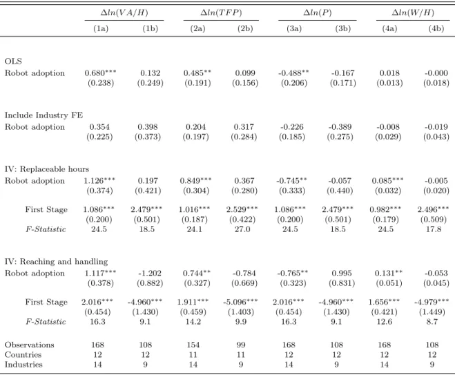
Estimation results are presented in Table 2. Looking at the results of the two productivity measures labor productivity (columns 1a and 1b) and TFP (columns 2a and 2b), we find that the OLS results for the full-sample are largely unchanged in comparison to Table 1, while the coefficients for the manufacturing sample are much larger, with the coefficient for the TFP estimation even being significant at the 10%

level. The inclusion of industry fixed effects, however, still leads to movements in the estimates which are similar to before, suggesting that our expanded set of controls still does not capture the full extend of unobserved industry specific heterogeneity.

6Also, we include initial period skill shares in the wage regression (instead of changes). This is a deviation from G&M (2018) as well as our wage regressions in columns 4a and 4b of Table1. We do this, because the changes in these skill shares are treated explicitly as a separate outcome in other regressions. Therefore, they are to be considered as a ‘bad control’ in the sense ofAngrist and Pischke (2008).

(19)

Table2:FullSample(a)vs.Manufacturing-onlySample(b)-IncludingAdditionalControlVariables: ShareinHoursWorkedbySkillGroup ∆ln(VA/H)∆ln(TFP)∆ln(P)∆ln(W/H)HighMiddleLow (1a)(1b)(2a)(2b)(3a)(3b)(4a)(4b)(5a)(5b)(6a)(6b)(7a)(7b) OLS Robotadoption0.650∗∗∗0.2670.442∗∗0.270∗-0.487∗∗-0.290∗0.035∗-0.0043.362∗∗∗1.0833.539∗-1.278∗∗-6.901∗∗∗0.195 (0.241)(0.202)(0.186)(0.160)(0.197)(0.151)(0.019)(0.026)(1.215)(0.898)(2.070)(0.625)(1.942)(0.952) IncludeIndustryFE Robotadoption0.3210.4520.1950.413-0.211-0.4300.008-0.0092.6401.8962.447-2.032∗∗-5.087∗0.136 (0.223)(0.356)(0.192)(0.312)(0.186)(0.267)(0.036)(0.056)(1.820)(1.622)(2.619)(0.918)(2.951)(0.960) IV:Replaceablehours Robotadoption1.203∗∗∗0.616∗∗0.909∗∗∗0.668∗∗∗-0.876∗∗∗-0.4110.088∗∗-0.022∗4.333∗∗0.4889.376-0.789-13.709∗∗∗0.301 (0.309)(0.295)(0.216)(0.250)(0.287)(0.344)(0.036)(0.013)(2.124)(0.711)(5.937)(1.198)(4.874)(1.160) FirstStage1.258∗∗∗2.297∗∗∗1.202∗∗∗2.260∗∗∗1.258∗∗∗2.297∗∗∗1.345∗∗∗2.195∗∗∗1.225∗∗∗2.236∗∗∗1.225∗∗∗2.236∗∗∗1.225∗∗∗2.236∗∗∗ (0.199)(0.453)(0.196)(0.487)(0.199)(0.453)(0.206)(0.451)(0.214)(0.414)(0.214)(0.414)(0.214)(0.414) F-Statistic32.518.830.315.632.518.833.916.726.421.126.421.126.421.1 IV:Reachingandhandling Robotadoption1.290∗∗∗-0.6370.906∗∗∗-0.755-0.926∗∗∗0.4910.133∗∗∗0.0096.904∗∗∗1.588∗∗6.271-4.271∗∗-13.176∗∗2.683∗∗ (0.335)(0.713)(0.257)(1.170)(0.274)(0.657)(0.036)(0.046)(2.498)(0.743)(6.010)(1.758)(5.445)(1.239) FirstStage2.162∗∗∗-4.522∗∗∗2.060∗∗∗-3.176∗∗∗2.162∗∗∗-4.522∗∗∗2.017∗∗∗-5.721∗∗∗2.062∗∗∗-5.786∗∗∗2.062∗∗∗-5.786∗∗∗2.062∗∗∗-5.786∗∗∗ (0.402)(1.185)(0.392)(0.873)(0.402)(1.185)(0.467)(1.575)(0.436)(1.460)(0.436)(1.460)(0.436)(1.460) F-Statistic23.510.622.19.623.510.614.99.318.111.418.111.418.111.4 Observations16810815499168108168108168108168108168108 Countries1212111112121212121212121212 Industries149149149149149149149 Note:∗<0.10,∗∗<0.05,∗∗∗<0.01.Robuststandarderrorsgroupedbycountryandeconomicsectorareshowninbrackets.Allvariablesarespecifiedingrowthratesorthepercentileof growth(robotdensity).Allspecificationscontaincountryfixedeffects,aswellasallcontrolvariablesfromGraetzandMichaels(2018).Additionally,allestimationscontrolforthe demographicstructureoftheworkforce.Allregressionsareweightedbythecountryspecificshareofsectoralemploymentintheinitialperiod(1993).

(20)

Also for the 2SLS estimations using the replaceable hours instrument, we find that estimates for the full sample are of comparable magnitude to before, while in the manufacturing sample estimates drastically increase in size and precision. These estimates are now both sizable and significant, indicating a positive impact of robotization on labor productivity and TFP.⁷ This also supports the results from G&M (2018), who also conclude that robotization leads to increases in productivity.

The results for output prices are very similar to those in Table 1, with the full sample results being largely unchanged and the estimates for the manufacturing sample pointing in the same direction, but lacking statistical significance.

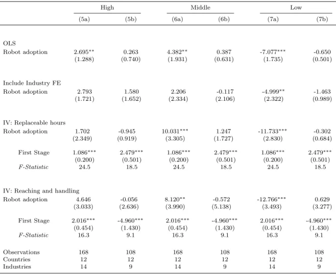
We next turn to the discussion of labor market outcomes. Again the results for wages in the full sample are largely the same as before, indicating positive wage effects of robotization. Looking at the manufacturing sample, we again find a negative coefficient, which is insignificant in the OLS and FE estimations, but is significant at the 10% level in the 2SLS estimation. With regard to the skill-composition of the labor force we find a clearly different picture to before. While the results for the full sample still indicate a decline in the share of low skilled workers, the manufacturing sample gives a different picture. Here the OLS and industry FE estimations yield statistically significant, negative estimates in the middle of the skill distribution, while at the top and bottom we find positive, albeit insignificant coefficients. This pattern resembles the well established result of job polarization that has been found by numerous studies examining the labor market impacts of automation.⁸ While the estimates for 2SLS

7To be sure that this result is not driven by the reduction in sample size, due to the limited availability of the demographic control variables, Online Appendix B re-estimates the results from Table1using only observations that can be used for the estimations in Table2.

8See for example Goos and Manning(2007),Autor, Katz, and Kearney(2008), Dustmann, Lud- steck, and Sch¨onberg(2009),Autor and Dorn(2013), orGoos, Manning, and Salomons(2014)

(21)

using the replaceable hours instrument do point in the same direction, these estimates are no longer significant. Therefore we have to regard this result as inconclusive. How- ever, we do not find evidence supporting employment losses at the bottom of the skill distribution.

To summarize, the inclusion of demographic controls yields positive effects of robotization on productivity, also when exclusively focusing on manufacturing sectors. With regard to labor market outcomes, we conclude that we are not able to detect positive wage effects and employment reductions for low-skilled workers as in G&M (2018). If anything, the data suggest the opposite. Our estimates point in the direction of negative effects on wages and job polarization (i.e. employment declines in the middle of the skill distribution).

Furthermore, while controlling for the demographic composition of the workforce yields significantly positive effects of robotization on both productivity measures, the coefficient movements resulting from the inclusion of industry fixed effects raise concerns that we still face some degree of unobserved heterogeneity, which biases the estimates.

This would not be a problem for the 2SLS estimation, if the instrument is exogenous to remaining unobserved confounders. However, the strong coefficient movements in the 2SLS estimation between Table1 and Table 2casts some doubt on whether this is the case. Rather, this picture is consistent with the view expressed in Altonji, Elder, and Taber(2005) andOster(2019), who state that coefficient movements, which are caused by the inclusion of observed control variables, hint at the importance of unobserved variables. They stress the fact that this is of particular importance, if the included measures are imperfect proxies, which might capture only part of the relevant process.

This is very likely the case with the included shares of middle-aged and old workers, as, following Acemoglu and Restrepo (2018), it is not the age composition per se that influences automation, but rather the more frequent prevalence of automatable skills

(22)

in middle-aged workers. Clearly this is imperfectly captured by the (rather crude) measures of age composition in the EU-KLEMS data. So while the inclusion of these additional controls should somewhat reduce endogeneity concerns, it is very likely not sufficient to fully eliminate them.

3.3 Extended Period: 2008-2015

In this section we present results for the period 2008-2015. Since all variables re- lating to workforce characteristics (i.e. skill-, age-, or gender-shares) only vary on the 1-digit industry level in the EU-KLEMS September 2017 release, we are not able to run regressions examining the impact of robotization on the skill-composition of the workforce, as these variables show no variation in the manufacturing sample. Furthermore, we are not able to additionally control for the skill-shares in the wage regression, or run additional regressions controlling for the demographic structure of the workforce.

Table 3shows our estimation results. Again we report estimates for the full sample in columns indicated with (a), and estimates for the manufacturing sample in columns indicated with (b). Comparing these results to the period 1993-2007 in Table 1 shows that all estimates are considerably smaller in the 2008-2015 sample. The OLS estimates and the industry fixed effects estimations are across the board very small, and generally much closer to zero than in the 1993-2007 estimations.

The 2SLS estimation, using the replaceable hours instrument, for labor productivity (columns 1a and 1b) and TFP (columns 2a and 2b) demonstrates that also in the full- industry sample estimates are very small and statistically insignificant. As before, the size of these estimates is even further reduced, when restricting to the manufacturing sample. In any case, we find no evidence for positive effects of robotization on productivity. For the change in output prices (columns 3a and 3b), the 2SLS estimates using the replaceable hours instrument point in the same direction as for the 1993-2007 sam-

(23)

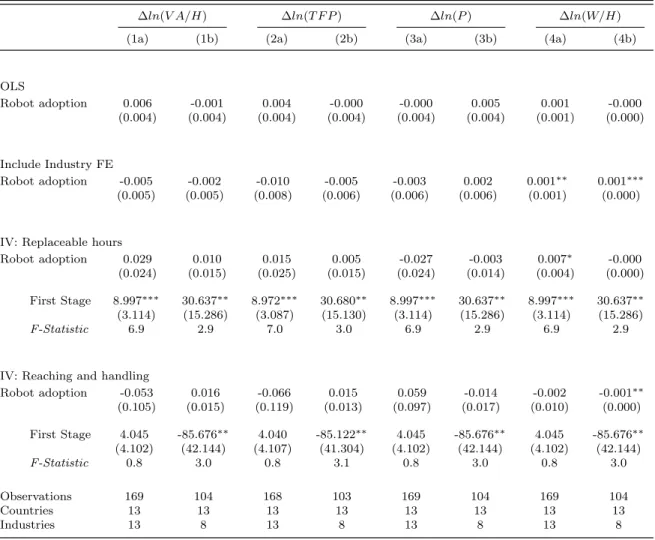
Table 3: Full Industry Sample (a) vs. Manufacturing-only (b) - Estimates for the Period 2008-2015

∆ln(V A/H) ∆ln(T F P) ∆ln(P) ∆ln(W/H)

(1a) (1b) (2a) (2b) (3a) (3b) (4a) (4b)

OLS

Robot adoption 0.006 0.017 -0.037 0.018 -0.023 -0.000 0.015^∗ -0.004

(0.109) (0.061) (0.126) (0.068) (0.068) (0.074) (0.008) (0.004)

Include Industry FE

Robot adoption -0.089 0.029 -0.129 0.022 0.010 -0.054 0.010 -0.002

(0.078) (0.074) (0.082) (0.061) (0.038) (0.081) (0.007) (0.002)

IV: Replaceable hours

Robot adoption 0.189 0.085 0.096 0.043 -0.175 -0.029 0.043^∗ -0.002

(0.169) (0.131) (0.171) (0.131) (0.153) (0.117) (0.024) (0.002)

First Stage 1.399^∗∗∗ 3.538^∗∗∗ 1.402^∗∗∗ 3.540^∗∗∗ 1.399^∗∗∗ 3.538^∗∗∗ 1.399^∗∗∗ 3.538^∗∗∗

(0.232) (0.893) (0.227) (0.881) (0.232) (0.893) (0.232) (0.893)

F-Statistic 30.2 11.5 31.6 11.8 30.2 11.5 30.2 11.5

IV: Reaching and handling

Robot adoption -0.082 0.191 -0.103 0.170 0.092 -0.164 -0.003 -0.007^∗

(0.153) (0.146) (0.184) (0.130) (0.125) (0.170) (0.017) (0.004)

First Stage 2.606^∗∗∗ -7.295^∗∗∗ 2.607^∗∗∗ -7.269^∗∗∗ 2.606^∗∗∗ -7.295^∗∗∗ 2.606^∗∗∗ -7.295^∗∗∗

(0.423) (2.114) (0.422) (2.084) (0.423) (2.114) (0.423) (2.114)

F-Statistic 31.5 8.7 31.6 8.9 31.5 8.7 31.5 8.7

Observations 169 104 168 103 169 104 169 104

Countries 13 13 13 13 13 13 13 13

Industries 13 8 13 8 13 8 13 8

Note: ∗<0.10,∗∗<0.05,∗ ∗ ∗<0.01. Robust standard errors grouped by country and economic sector are shown in brackets. All variables are specified in growth rates or the percentile of growth (robot density). All specifications

contain country fixed effects, as well as all control variables fromGraetz and Michaels(2018). All regressions are

weighted by the country specific share of sectoral employment in the initial period (2008).

ple, with both coefficients being negative. The estimate for the manufacturing sample is however less than half as big as in table1 and statistically not distinguishable from zero. The only significant estimate in the full sample is found for changes in average wages, where the 2SLS estimation indicates a positive relationship between robotization and average wages. When restricting the sample to manufacturing industries, this positive coefficient again turns negative, and lacks statistical significance. Hence, when

(24)

applying the setting of G&M (2018) on the period 2008-2015, we are not able to detect any impact of robotization on productivity, prices or wages. This could be interpreted as an indication that the main impacts of robotization, at least on an aggregate industry level, have already taken place by 2008.

Looking closer at the two instruments that are used, we see that the replaceable hours instrument is weaker, when applied to the 2008-2015 period, but still exceeds the commonly used threshold of an F-statistic greater 10. For the reaching and handling instrument we find the same reversal of direction in the first-stage coefficient as in the 1993-2007 sample, indicating again towards a violation of the monotonicity assumption.

Therefore, we regard this as further evidence that the reaching and handling instrument should not be regarded as reliable, and therefore future research should refrain from using it.

4 Discussion and Conclusion

This paper reveals pitfalls in the use of the IFR robot data at the industry level, which is currently the most prominent source for automation research in economics. In doing so, we reassessed the effects of robotization on productivity, prices, wages and the skill-composition of the workforce. We thereby restricted the sample of used country- industry observations to manufacturing industries only, motivated by the fact that these sectors are almost exclusively affected by robotization. This restriction results in insignificant estimates across the board. In an effort to control more thoroughly for unobserved industry level heterogeneity, we include the demographic composition of the workforce into our regressions. Doing this leads to sizable and significant effects of robotization on productivity.

However, regarding the remaining outcomes, we have to reject the hypothesis that

(25)

robotization causes skill-biased technological change or positive wage effects. Rather the opposite, falling wages and job polarization, is the case. Our analyses provide clues in this direction, but we do not get robust results across all specifications. Our results support the idea that the aging process is closely connected to automation, as put forward byAcemoglu and Restrepo(2018) orDauth et al.(2021). In a further step, we repeated all estimations for the extended period 2008-2015, where we are again unable to detect any significant effects of robotization on productivity, prices, or wages.⁹ We interpret this as an indication that the effects of robotization weaken over time, at least at the aggregate level. Current research at the firm level (e.g. Koch, Manuylov, and Smolka(2019),Acemoglu, Lelarge, and Restrepo(2020) orBonfiglioli et al.(2020)) still shows considerable positive economic outcomes for robotizing firms as well as negative spillovers for non-adopters in recent periods. However, if one takes into account the low prevalence of robotizing firms across all industries,¹⁰ there are not necessarily any substantial positive or negative effects for the economy as a whole. Additionally, a critical appraisal of the actual, disruptive potential of current robot technology is also helpful in interpreting our findings. It is an open question whether the currently existing robot technology actually represents a break with known automation technologies or is not rather an iteration of the same, the greatest impact of which has already taken place long ago (Fernandez-Macias, Klenert, and Anton, 2020). Accordingly, by following the benchmarking procedure of G&M (2018) we estimate that in the absence of changes

9Unfortunately, EU-KLEMS as an important source of data on productivity and employment, no longer allows to control for demographic factor at the current data edge and thus these extended results suffer from unobserved heterogeneity.

10Deng, Pl¨umpe, and Stegmaier(2020) show for Germany, one of the most robotized countries, that overall only 1.55% of all plants use robots. While this figure rises to 8.22% for manufacturing, even in the most robot-intensive manufacturing industries (motor vehicles and plastics) three-quarters of plants do not use any robots.

(26)

in robotiziation, productivity in the overall economy would have been only around 2%

lower in 2007, compared to an estimated productivity effect of 5% in G&M (2018).¹¹ Finally, an important result concerns the validity of one of instruments used to study automation. G&M (2018) proposed one instrument based on the prevalence of reaching and handling tasks in an industry. Here, we find a concerning reversal of the sign of the first-stage coefficient for this ‘reaching and handling’ instrument, when restricting the sample to manufacturing industries only. In our view, this provides evidence that this instrument does not satisfy the monotonicity assumption. We therefore advise caution when using this instrument, as it potentially distorts results leading to questionable inference. This point is of particular importance, as several papers have already used this instrument in various contexts.

11For this benchmark we followed the procedure described in the Online-Appendix of Graetz and Michaels(2018). This procedure is based on a coefficient from an OLS estimation controlling only for country and industry specific trends. Using the manufacturing only sample, this estimated coefficient is 0.358, which implies a productivity increase in the overall economy of around 2% between 1993 and 2007. If we use our preferred estimate of 0.616 from table2, column 1b (using the replaceable hours instrument and a full set of controls), we estimate that productivity in the overall economy would have been approximately 4% lower in the absence of robotization. We want to note here, that including low-robotization probability industries in the 2SLS estimation with all controls used by G&M (2018) (which results in an estimate of 1.051 - see table1, column 1a) implies an unreasonably high impact of robotization on the average level of productivity in the overall economy of around 12%. We regard this as further evidence, that low-robotization probability sectors should be excluded, when conducting this type of analysis.

(27)

References

Acemoglu, Daron, Claire Lelarge, and Pascual Restrepo. 2020. “Competing with Robots: Firm-Level Evidence from France.” AEA Papers and Proceedings 110:383–

88.

Acemoglu, Daron and Pascual Restrepo. 2018. “Demographics and Automation.” Tech.

rep., National Bureau of Economic Research, Cambridge, MA.

———. 2020. “Robots and Jobs: Evidence from US Labor Markets.” Journal of Political Economy 128 (6):2188–2244.

Aksoy, Cevat Giray, Berkay ¨Ozcan, and Julia Philipp. 2020. “Robots and the Gender Pay Gap in Europe.” IZA Discussion Paper 13482.

Altonji, Joseph G., Todd E. Elder, and Christopher R. Taber. 2005. “Selection on Observed and Unobserved Variables: Assessing the Effectiveness of Catholic Schools.”

Journal of Political Economy 113 (1):151–184.

Angrist, Joshua D. and J¨orn-Steffen Pischke. 2008. Mostly Harmless Econometrics: An Empiricist’s Companion. Princeton University Press.

Autor, David H. and David Dorn. 2013. “The Growth of Low-Skill Service Jobs and the Polarization of the US Labor Market.” American Economic Review 103 (5):1553–

1597.

Autor, David H., Lawrence F. Katz, and Melissa S. Kearney. 2008. “Trends in U.S.

Wage Inequality: Revising the Revisionists.” The Review of Economics and Statistics 90 (2):300–323.