Decision Maps for Bivariate Time Series with Potential Threshold Cointegration

IHS Economics Series Working Paper 121

September 2002

Decision Maps for Bivariate Time Series with Potential Threshold Cointegration

Robert M. Kunst

Impressum Author(s):

Robert M. Kunst Title:

Decision Maps for Bivariate Time Series with Potential Threshold Cointegration ISSN: Unspecified

2002 Institut für Höhere Studien - Institute for Advanced Studies (IHS) Josefstädter Straße 39, A-1080 Wien

E-Mail: o ce@ihs.ac.atffi Web: ww w .ihs.ac. a t

All IHS Working Papers are available online: http://irihs. ihs. ac.at/view/ihs_series/

Decision Maps for Bivariate Time Series with Potential Threshold Cointegration

Robert M. Kunst

121

Reihe Ökonomie

Economics Series

121 Reihe Ökonomie Economics Series

Decision Maps for Bivariate Time Series with Potential Threshold Cointegration

Robert M. Kunst

September 2002

Contact:

Robert M. Kunst University of Vienna and

Institute for Advanced Studies Department of Economics

Stumpergasse 56, A-1060 Vienna, Austria (: +43/1/599 91-255

email: kunst@ihs.ac.at

Founded in 1963 by two prominent Austrians living in exile – the sociologist Paul F. Lazarsfeld and the economist Oskar Morgenstern – with the financial support from the Ford Foundation, the Austrian Federal Ministry of Education and the City of Vienna, the Institute for Advanced Studies (IHS) is the first institution for postgraduate education and research in economics and the social sciences in Austria.

The Economics Series presents research done at the Department of Economics and Finance and aims to share “work in progress” in a timely way before formal publication. As usual, authors bear full responsibility for the content of their contributions.

Das Institut für Höhere Studien (IHS) wurde im Jahr 1963 von zwei prominenten Exilösterreichern – dem Soziologen Paul F. Lazarsfeld und dem Ökonomen Oskar Morgenstern – mit Hilfe der Ford- Stiftung, des Österreichischen Bundesministeriums für Unterricht und der Stadt Wien gegründet und ist somit die erste nachuniversitäre Lehr- und Forschungsstätte für die Sozial- und Wirtschafts - wissenschaften in Österreich. Die Reihe Ökonomie bietet Einblick in die Forschungsarbeit der Abteilung für Ökonomie und Finanzwirtschaft und verfolgt das Ziel, abteilungsinterne Diskussionsbeiträge einer breiteren fachinternen Öffentlichkeit zugänglich zu machen. Die inhaltliche

Abstract

Bivariate time series data often show strong relationships between the two components, while both individual variables can be approximated by random walks in the short run and are obviously bounded in the long run. Three model classes are considered for a time-series model selection problem: stable vector autoregressions, cointegrated models, and globally stable threshold models. It is demonstrated how simulated decision maps help in classifying observed time series. The maps process the joint evidence of two test statistics: a canonical root and an LR--type specification statistic for threshold effects.

Keywords

Model selection, Bayes testing, nonlinear time series models

JEL Classifications

C11, C15, C32

Comments

The data on U.S. interest rates are taken from the International Financial Statistics database. The

Contents

1 Introduction 1

2 Designing the simulation 4

2.1 Decision maps ...4

2.2 The model hypotheses ...6

2.3 The discriminatory statistics... 10

2.4 Smoothing ... 11

3 Simulation results: the maps 12

4 Summary and conclusion 21

Appendix:

Geometric ergodicity of threshold cointegrated models 23

References 25

1 Introduction

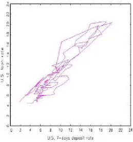
Bivariate time series data often exhibit features like the pair of retail interest rates in Figure 1. The two component series appear to be closely linked such that deviations from each other are relatively small. For long time spans, the variables move up or down the positive diagonal, with very little memory with respect to this motion. Individually, the series appear to be well described as random walks or at least as …rst-order integrated processes with low autocorrelation in the di¤erences. Eventually, however, the upward or downward motion seemingly hits upon some outer boundary and is reversed, such that all observations are contained in a bounded interval, in the long run. The bounds of the interval are assumed as unknown. A good example for such pairs of time series data are interest rates, such as saving and loan rates or bill and bond rates, though a deep economic analysis of interest rates is outside the scope of this paper. We just observe that they attain their maximum in phases of high in‡ation and that their minimum is usually strictly positive.

Figure 1: Time-series scatter plot of monthly data on U.S. interest rates on loans and 7-days deposits, 1963–2002.

This paper is concerned with selecting an appropriate time series model

for data such as the depicted series, if the set of available classes is given by

the three following ideas. Firstly, the observed reversion to some distribu- tional center may suggest a linear stable vector autoregression. This model class has the drawback that the autoregression is unable to re‡ect the random movement in the short run. Secondly, this movement and the obvious link between the components may suggest a cointegrated vector autoregression.

Particularly for interest rates of di¤erent maturity, this is an idea that ap- pears in the econometric literature, see for example Campbell and Shiller (1987), Hall et al. (1992), or Johansen and Juselius (1992). Enders and Siklos (2001) even state that “it is generally agreed that interest-rate series are I(1) variables that should be cointegrated”. The drawback of this model class is that it is unable to match the long-run boundedness condi- tion. The model contains a unit root, is non-ergodic and inappropriate from a longer-run perspective (see Weidmann, 1999, for a similar argument in economics). Thirdly, one may consider a mixture of the two models, with cointegration prevailing in a ‘normal’ regime and global mean reversion in an ‘outer’ regime. This idea yields a threshold cointegration speci…cation, as it was used by Jumah and Kunst (2002), again for interest rates. The drawback of the model is that it is nonlinear and that it contains some poorly identi…ed parameters.

The concept of threshold cointegration is due to Balke and Fomby (1997, henceforth BF) who assumed a version with cointegration in the outer regime and an integrated process without cointegration in an inner regime.

Jumah and Kunst (2002) suggested a modi…cation of BF’s model that

is in focus here. Threshold cointegration models were also considered by

Enders and Granger (1998), Enders and Falk (1998), and Enders

and Siklos (2001). These contributions focus on asymmetric adjustment

to disequilibrium and hence they mainly use two-regime or single-threshold

models. Hansen and Seo (2002) analyze hypothesis testing for single-

threshold cointegration models and assume cointegration in both regimes,

though with di¤erent cointegrating vectors. Like BF, Lo and Zivot (2001)

consider the case of three regimes, with cointegration in the lower and upper

regimes and no cointegration in the central regime. While these authors allow

for asymmetric reaction or di¤erent cointegrating structures across regimes,

only symmetric reaction outside the band will be considered here, due to

the limited information that is provided by the few observations in the outer

region of our models. Weidmann (1999) analyzed bivariate time series of

an in‡ation index and an interest rates and suggested a three-regimes model

that is close to the one used here. Whereas his model assumes di¤erent

cointegration structures across regimes and achieves global stability by the choice of cointegrating vectors in the outer regimes, we impose local stability in the outer regimes. Tsay (1998) considered related models in a more general framework. His example of ‡ow data for two Icelandic rivers may also conform to the pattern of Figure 1, as the ‡ow is bounded from below by zero and from above by some natural maximum.

Threshold cointegration models are particular threshold vector autore- gressions of the SETAR (self-exciting threshold autoregression) type that was considered by Chan et al. (1985), Tong (1990), Chan (1993), and Chan and Tsay (1998). Particularly Chan et al. (1985) found that stability in the outer regimes is su¢cient, though not necessary, for global stability and geometric ergodicity. It follows that the models suggested here are globally stable and geometrically ergodic. To the author’s knowledge, the proof of this important property has not been given explicitly in the literature. It has been added to this paper as an appendix.

Each of the three outlined model classes deserves attention as a possi- ble data-generating mechanism. It is therefore interesting to study methods that allow selecting among the classes on the basis of observed data. The decision set consists of three elements: the stable vector autoregression, the linear cointegration model, and the threshold cointegration model. Candi- dates for discriminatory statistics are likelihood ratios for any two of these model classes or approximations thereof. The theory of likelihood ratios be- tween the …rst and the second class has been developed by Johansen (1988), hence it is convenient to include this ratio in the vector statistic. As another statistic, we add an approximation to the likelihood ratio of the …rst and the third class.

Model selection is a …nite-action problem and requires procedures beyond

the dichotomy of the standard Neyman-Pearson framework of null and alter-

native hypotheses. Here, the three competing model classes are modeled as

three alternative Bayes data measures. Each measure can be conditioned on

the values of a vector statistic, such that the probability for each hypothesis

can be evaluated conditional on the given or observed test statistic. The

model or hypothesis with maximum probability is then the suggested choice

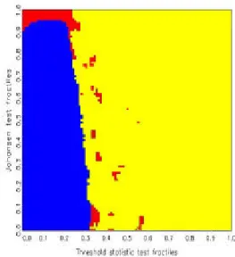
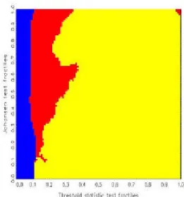
for the observed value of the statistic. In the space of null fractiles of the test

statistics, one obtains ‘decision maps’ that show distinct regions of preference

for each model class. This approach builds on a suggestion by Hatanaka

(1996) and was used by Kunst and Reutter (2002), among others. For

the present problem, non-informative prior distributions are elicited on the

basis of Jordan distributions (see also Kunst, 2002). Discrete uniform priors over the three hypotheses are allotted implicitly. All calculations of decision maps have been conducted by means of simulation. Decision maps are par- ticularly well suited for model selection based on the joint evaluation of two test statistics.

The remainder of this paper is structured as follows. Section 2 explains the decision maps approach and details the properties of the entertained models, including the elicitation of non-informative prior distributions. Sec- tion 3 reports the simulation results, including the maps and their tentative interpretation. Section 4 concludes.

2 Designing the simulation

2.1 Decision maps

The decision maps approach can be applied to all parameterized problems (f

; µ 2 £) for …nite-dimensional £, where a decision is searched among a

…nite number of rival hypotheses (a partition of £), preferably on the basis of a bivariate vector statistic. For a univariate statistic, the maps collapse to intervals on the real line. For vector statistics with a higher dimension, the visual representation of the maps encounters technical di¢culties.

Assume a decision concerns the indexed set of hypotheses f H

= f µ 2 £

g , j = 1; : : : ; h g . Usually, model selection utilizes h ¡ 1 likelihood-ratio statistics S

or approximations thereof, for ‘null’ hypothesis H

and alternative H

, with 1 · j < h, 1(j) 6 = 2(j), and 1(j), 2(j ) 2 f 1; : : : ; h g . For ease of notation, let these statistics be collected in an h ¡ 1–dimensional vector sta- tistic S = (S

; : : : ; S

)

, such that S

and S

can be used equivalently.

The classical approach requires nested hypotheses, such that £

½ £ ¹

, where bars denote topological closure. If parameter sets can be completely ordered, one may write £

½ £ ¹

for 1 · j < h. Then, two typical choices of vector likelihood-ratio statistics are S = (S

; S

; : : : S

)

and S = (S

; S

; : : : ; S

)

.

Let weighting prior distributions be de…ned on each £

, 1 · j · h by their densities ¼

. For any pair (1(j ); 2(j)), 1 · j < h, the collection of distributions ¡

f

; µ 2 £

¢ de…nes a null distribution f

of the statistic S

via the implied p.d.f. of this statistic under µ, denoted as f

by Z

£j1

f

(x)¼

(µ)dµ = f

(x) : (1) Note that it is equally possible to de…ne a null distribution f

of the very same statistic. Let F

denote the c.d.f. that corresponds to f

. Then, the preference area for £

is de…ned by

P A

= f z = (z

; : : : ; z

)

2 (0; 1)

j j = arg max

j

P (H

j S ) ;

z

= F

(S

) g : (2)

The transformation F

serves to represent the preference areas conveniently in a simplex instead of some possibly unbounded subspace of R

. A graph- ical representation of preference areas is called a decision map.

The meaning of (2) can be highlighted by considering its counterpart in classical statistics. Suppose h = 3, and two statistics are evaluated. In a (0; 1)

–diagram for the fractiles of the null distributions for S

and S

, a given sample of observations de…nes a point of realized statistics. Classical statistics would base its decision on rejections in a test sequence, for example starting from the more general decision on S

. If one-sided tests are used that reject for the upper tails of their null distributions, the classical preference area for hypothesis £

or H

is the rectangle A

= (0; 1) £ (0:95; 1). If £

is not rejected, test S

will be applied and separates the preference areas for

£

, A

= (0; 0:95) £ (0; 0:95), and for £

, A

= (0:95; 1) £ (0; 0:95). Classical statistics may face di¢culties in uniquely determining the null distributions, as fractiles usually vary within each collection. The (0; 1)

–chart split into the three rectangles constitutes a classical decision map.

Bayesian decision maps are more complex than classical decision maps, as the boundaries among the preference areas may be general curves. Excepting few simple decision problems, it is di¢cult to calculate the value of a condi- tional probability for a given point of the (0; 1)

–square in the fractile space.

It is more manageable to generate, by numerical simulation, a large number of statistics from the priors with uniform weights across the hypotheses and to collect the observed statistics in a bivariate grid over the fractile space.

Within each ‘bin’, the maximum of the observed values can be evaluated

easily. In computer time, the simulation can be time-consuming but requires

little more storage than hg

, where h is the number of considered hypotheses

and g is the inverse resolution of the grid, i.e., there are g

bins.

In summary, numerical calculation of a decision map consists of the fol- lowing steps: …rst, a conveniently large number of replications for each of the two statistics under their respective null distributions are generated; sec- ond, a grid of fractiles are calculated from the sorted simulated data; third, both statistics are generated from any of the competing hypotheses, i.e., from the prior distributions ¼

. These statistics are allotted into the bins as de-

…ned by the fractiles grid. Finally, each bin is marked as ‘belonging’ to that hypothesis from which it has collected the maximum number of entries.

The simulation of the null fractiles requires a number of replications that is large enough to ensure a useful precision of the fractiles. For the purpose of the graphical map, a high precision may not be required. If the map is intended for usage in later applications, it may also be convenient to replace the exact null distribution by an approximation, particularly if that approx- imation is a standard distribution that allows an evaluation in a closed form.

If the null fractiles indeed have to be simulated, a large number of replica- tions slows down the simulation considerably due to the sorting algorithm that is applied in order to determine empirical fractiles.

By contrast, a fairly large number of replications can be attained for the simulation of statistics conditional on the respective hypotheses. Computer time is limited by the calculation time of the statistics only, which may take time if some iteration or non-linear estimation is required, while only a g £ g matrix of bins for each hypothesis is stored during the simulation. For g = 100, 10

replications yield acceptable maps. For h hypotheses, this gives 10

¢ h replications. It was found that kernel smoothing of the bin entries improves the visual impression of the map more than considerably increasing the number of replications (see Section 2.4).

2.2 The model hypotheses

For model selection, prior distributions with point mass on lower-dimensional parameter sets are required. Then, ‡at or Gaussian distributions are used on the higher-dimensional sets, with respect to a convenient parameterization.

The speci…c requirements of decision map simulations rule out improper or

Je¤reys priors, hence the priors do not coincide with the suggestions for unit-

root test priors in the literature (see Bauwens et al., 1999). They are maybe

closest to the reference priors of Berger and Yang (1994), that peak close

to the lower-dimensional sets and are relatively ‡at elsewhere.

The …rst model H

is the stable vector autoregression µ x

y

¶

= ¹ + X

j=1

©

µ x

y

¶ +

µ "

"

¶

(3) with all zeros of the polynomial Q (z) = det(I ¡ P

j=1

©

z

) outside the unit circle. For p = 1, this condition is equivalent to the condition that all latent values of © = ©

have modulus less than one. This again is equivalent to the property that © has a Jordan decomposition

© = TJT

(4)

with non-singular transformation matrix T and ‘small’ Jordan matrix J. If one restricts attention to real roots and to non-derogatory Jordan forms, the matrix J is diagonal with both diagonal elements in the interval ( ¡ 1; 1).

Therefore, the prior distribution for this model ¼

can be simply taken from the family of Jordan distributions and is de…ned by

t

; t

» N (0; 1) t

= t

= 1

j

; j

» U ( ¡ 1; 1)

"

= ("

; "

)

» N (0; I

); (5) where the notation J = (j

) etc. is used. The concept can be extended easily to the case p > 1 and to non-zero ¹. For the basic experiments, p = 1 and ¹ = 0 is retained. Unless otherwise indicated, all draws are mutually independent. For example, "

and "

are independent for s 6 = t in all experiments, thus assuming strict white noise for error terms.

This prior distribution is not exhaustive on the space of admissible mod- els. It excludes derogatory Jordan forms and complex roots. Derogatory Jordan forms are ‘rare’ in the sense that they occupy a lower-dimensional manifold. Complex roots are covered in an extension that was used for some experiments. In this variant, 50% of the © matrices were drawn from

© = TJ

T

instead of (4), with J

=

µ r cos Á r sin Á

¡ r sin Á r cos Á

¶

: (6)

It is known from matrix algebra that J

is obtained from an original diagonal 2 £ 2–matrix J with conjugate complex elements that is transformed by a complex matrix

T

=

µ 1 + i 1 ¡ i 1 ¡ i 1 + i

¶

(7) such that J

= T

JT

. The prior distribution for J

is constructed by drawing r from a U (0; 1) distribution and Á from a U(0; ¼) distribution. The speci…cation for the priors for T is unchanged. For these experiments with complex roots, also the prior distribution for H

was modi…ed accordingly.

In H

, both variables x and y have a …nite expectation and revert to it geometrically. In geometric terms, the (x; y)–plane has a unique equilibrium point (¹ x; y), which in the case ¹ ¹ = 0 collapses to (0; 0).

The second model class H

consists of cointegrating vector autoregres- sions, with the cointegrating vector de…ned as the di¤erence of the two vari- ables (1; ¡ 1). For interest rates of di¤erent maturity, this di¤erence is the

‘yield spread’. For saving and loan rates, it is the mark-up of banks. For

…rst-order vector autoregressions of this type, a prior distribution is obtained from the error-correction representation

µ ¢x

¢y

¶

= ¹ + ¦

µ x

y

¶ +

µ "

"

¶

(8) with a matrix ¦ of rank one. The matrix ¦ can be represented in the form

¦ = µ ®

®

¶

(1; ¡ 1) : (9)

The elements ®

and ®

are chosen in such a way that explosive modes in the system are avoided. Again, this condition is more readily imposed on the Jordan representation ¦ = TJT

with diagonal matrix J = diag (¸; 0) for

¸ 2 ( ¡ 2; 0). The speci…cation

T =

µ 1 1 a 1

¶

(10) with a » N (0; 1) covers a wide variety of admissible matrices ¦. The implied form of ¦ is

¦ = 1 1 ¡ a

µ ¸ ¡ ¸ a¸ ¡ a¸

¶

(11)

and satis…es the general form (9). The class H

again assumes "

» N (0; 1) for the disturbances and, in the basic speci…cation, ¹ = 0. The thus de…ned prior ¼

is more di¢cult to generalize to higher p than ¼

.

The third model class H

are threshold cointegrating models. The basic form of these models is

µ ¢x

¢y

¶

= ¹ + µ ®

®

¶

(1; ¡ 1)

µ x

y

¶

+ µ ®

®

¶ (1; 0)

µ x

y

¶

I fj x

¡ » j > c g + µ "

"

¶ (12) : The symbol I f : g denotes the indicator function on the set f : g . There are two cointegrating vectors. The …rst one, (1; ¡ 1), is always active whereas the second one, (1; 0), is only activated at ‘large’ values of the trigger variable, in our case x

. An obvious variant is obtained by replacing the second vector by (0; 1) and the trigger variable by y

. We do not focus on the choice of the trigger variable, nor do we consider a variation of the trigger lag (‘delay’), as is common in the literature on threshold time series models.

The model is ergodic and both variables x and y have …nite expectation (see Appendix). The typical behavior is obtained if the mean implied by the

‘outer’ linear regime µ ¢x

¢y

¶

= ¹ +

µ ®

®

®

®

¶ µ 1 ¡ 1 1 0

¶ µ x

y

¶ +

µ "

"

¶

(13) is contained in the set C = fj x

¡ » j < c g . Then, the mean is targeted for ‘large’ values of x and, because of cointegration, also for large values of y, that imply large values of x. If the band C is reached, i.e., if x is

‘small’ again, the ‘outer’ mean is no longer interesting. Instead, the dynamic behavior of the variables resembles cointegrated processes, until the band is left and the cycle starts anew. Whenever the ‘outer’ mean falls outside the band, typical trajectories will remain near the ‘outer’ mean for long time spans. Only atypically large errors will shift them into the band, where cointegrated behavior takes over. In the …rst case, the intersection of C and the generic error-correction vector f (x; x) j x 2 Rg can be regarded as an

‘equilibrium’, with the error-correction vector possibly suitably shifted up or down by restrictions on ¹. In the second case, the implied mean of the outer regime constitutes a further element of the equilibrium or attractor set.

Hence, the threshold model allows for substantial variation in behavior.

In concordance with the other models, we do not elicit informative priors

but rather de…ne non-informative reference structures with stochastic para- meters. To this aim, we adhere to the following basic principle. Suppose we are given the traditional statistical problem of testing a point value against a

…nite interval. In that case, we would assume weights of 0.5 for each hypoth- esis and a uniform prior on the interval for the ‘alternative’. Treating the present problem in an analogous manner, we use a normal distribution for » and a half-normal distribution for c. These laws are su¢ciently ‡at around 0 to mimic the behavior of the typical uniform and normal laws. However, as a consequence of these assumptions, many processes show trajectories with little indication of threshold behavior. In fact, many trajectories closely resemble those drawn from the …rst model. Occasionally, ‘non-revealing’ tra- jectories occur if the threshold criterion is never activated in the assumed sample length. Statistical criteria cannot be expected to classify such cases correctly. In summary, it may be more di¢cult to discriminate H

from H

[ H

than to discriminate between H

and H

.

2.3 The discriminatory statistics

In order to discriminate among the three candidate models, two discrimi- natory statistics were employed. The statistic S

is designed to be power- ful in discriminating H

and H

. In the notation of section 2.1, it would be labelled S

. S

is de…ned as the smaller canonical root for (¢x

; ¢y

) and (x

; y

). As Johansen (1995) pointed out, this root makes part of the likelihood-ratio test for hypotheses that concern the cointegrating rank of vector autoregressions. If the larger canonical root is zero, (x; y) forms a bivariate integrated process without a stable mode. If only the smaller canonical root is zero, (x; y) is a cointegrated process with a stationary lin- ear combination ¯

x + ¯

y. If also the smaller canonical root is non-zero, (x; y) is a stationary process with all modes being stable. It was outlined above why the rank-zero model is not acceptable for interest rates. Hence, the smaller root is in focus.

The statistic to appear on the x–axis, S

, is designed to discriminate

H

and H

, hence in the notation of section 2.1 it would be labelled S

,

though it may also be useful in discriminating H

and H

. S

is an approx-

imate likelihood-ratio test statistic for the stationary vector autoregression

H

versus the quite special threshold-cointegrating model with c and » being

determined over a grid of fractiles of x. In detail, c is varied from the halved

interquartile range to the halved distance between the empirical 0.05 and

0.95 fractiles, with » thus assumed in the center of the range. For assumed models of type (12), the error sum of squares is minimized over a grid with step size of 0.05. As T ! 1 , this grid should be re…ned. Conditional on

» and c, estimating (12) is an ordinary least-squares problem with a corre- sponding residual covariance, whose log determinant can be compared to that of the unrestricted linear autoregression. The residual under the assumption of model class H

is denoted by ^ "

. For j = 1; 2, this residual is calcu- lated using the maximum-likelihood estimator. For j = 3, the approximate maximum likelihood estimator over the outlined grid is used. The residual covariance matrix is denoted by § ^

= T

P

t=1

^ "

^ "

. With this notation, the second statistic is de…ned as S

= ln ³

det ^ §

´ ¡ ln ³ det ^ §

´ .

Note that S

can be positive or negative. S

< 0 for strong nonlinear threshold e¤ects, as H

attains a better …t. S

> 0 for stable autoregres- sions. The hypotheses H

and H

are not nested. The statistic S

uses optimizing the likelihood ratio over a limited range, which is the prevalent approach for nonlinearity testing. An alternative is the semi-parametric test by Tsay (1998) that relies on sorting the observations according to the source of nonlinearity. The fully parametric nature of our decision problem suggests the use of S

, however.

The null fractiles were generated as follows. For S

, Jordan priors were used on a cointegrating autoregression—the classical lower-dimensional ‘null’

hypothesis H

. The cointegrating rank was …xed at one, whereas the cointe- grating vector was not speci…ed in constructing S

. The null fractiles di¤er from those that were tabulated by Johansen (1995), as those were calcu- lated under the hypothesis of multivariate random walks. For S

, Jordan priors on stable vector autoregressions were used, corresponding to the clas- sical ‘null’ hypothesis H

.

2.4 Smoothing

The technique of discretizing the statistics in bins corresponds to a rectangu-

lar smoothing kernel in density estimation. Similarly, simulated boundaries

of the decision areas often have a rough appearance, even for a high number

of replications. It was found that smoothing the original numbers in the bins

across neighboring bins is not so reliable as smoothing approximate poste-

rior probabilities for the hypotheses. This e¤ect is likely due to the scaling

of numbers. As a smoothing kernel, an inverse absolute function w (i; j) = W

1 + j i ¡ i

j + j j ¡ j

j ; i

¡ n

· i · i

+ n

;

j

¡ n

· j · j

+ n

(14) was used over an (2n

+ 1) £ (2n

+ 1) submatrix of the complete matrix of bins. This submatrix is centered at the location (i

; j

), where the value is to be estimated. W is set such that the sum of kernel weights P

w(i; j) over the submatrix equals one. As a general rule, the number n

was selected as the minimum number, at which smooth boundary curves were obtained.

The maps show some deliberate variation of n

, in order to demonstrate its in‡uence on the results.

3 Simulation results: the maps

Figures 2 and 3 show decision maps resulting from 3 £ 10

simulations of process trajectories of length T = 50 with stochastic parameters according to the prior distributions that were described in Section 2.2, i.e., 10

simulations for each model. In Figure 2, no smoothing was performed (n

= 0), while n

= 3 was set in Figure 3. In color coding, the preference area for the stationary autoregression H

is indicated in yellow (light gray), the one for the cointegrated autoregression H

in blue (dark gray), and for the threshold cointegrated model H

in red (medium gray). One sees that the main e¤ect of smoothing is a better separation of the preference areas for H

and H

, which is mainly achieved by eliminating the scattered preference specks for the rather inhomogeneous hypothesis H

. Further increases of n

distort the main boundaries of H

and H

and of H

and H

.

The main features of the decision map are somewhat surprising. The threshold statistic S

appears to be valuable in discriminating cointegrated and stable models, while it was designed to point out threshold structures.

The Johansen-type statistic S

separates linear cointegrated models from

cases of threshold cointegration, while it was designed to test for potential

cointegration in stable vector autoregressions. A closer look reveals that

H

models are indeed characterized by small values of S

, as expected, and

hence are most numerous in the left part of the chart. However, H

models

also incur small values of the statistic S

, as a threshold structure with the

critical value pushed away from the starting values will achieve a better …t

to data than an unrestricted vector autoregression for cointegrated models.

In other words, linear cointegration results as a limiting case of threshold cointegration. The posterior probability for H

is more concentrated than that for H

, hence H

dominates the left part of the diagram. Similarly, rejection of the smaller canonical root being zero may point to a stable linear model without unit roots but it may also point to a threshold model, which is stationary and ergodic though non-linear. The joint evidence of two non-zero canonical roots and a better …t by a restricted structure yields the preference area for H

in the north-west.

The map implies a crude empirical guideline. First, use the threshold statistic S

. For values larger than the 0.3 fractile, a linear stable model is suggested. For smaller values, use the lesser canonical root S

. If this root is ‘signi…cant’ at 0.05, consider the threshold model, otherwise opt for linear cointegration.

Figure 2: Decision map for processes without deterministic part. T = 50, n

= 0. The blue (dark) area prefers H

, the yellow (light) area prefers H

and the red (medium) area prefers H

. The same color code is used for the other …gures.

In Figure 4, the sample size has increased to T = 100, while the other

simulation parameters were retained. The smoothing bandwidth was kept at

Figure 3: Decision map for processes without deterministic part. T = 50, n

= 3.

n

= 3. The nominal signi…cance level of the canonical root has decreased to 0.02, whereas the critical fractile of the threshold statistic decreases to 0.2. These features are in line with expectations regarding large-sample per- formance. There is now more evidence on a preference for threshold models in a wedge between the other two models, i.e., for threshold statistics in the fractile range (0:2; 0:3), particularly if S

is ‘not too small’. The scattered appearance of the H

area re‡ects the varying shape of trajectories of length T = 100, which generally does not permit a safe classi…cation. Many of these H

trajectories are indeed very similar or identical to H

trajectories from the stable model class.

Figure 5 shows the map for T = 200. The critical fractile of S

for H

[ H

versus H

decisions shifts in to 0.12, while the implied signi…cance level of S

for H

versus H

decisions has fallen to 0.01. The boundary is

‡anked by an unconnected preference area for H

. Metaphorically speaking,

it looks as if the dark H

curtain were drawn from a window that reveals a

landscape that is populated by H

as well as H

models. Due to the large

variation in appearance of H

trajectories, the typical shape of the decision

map is likely to persist in even much larger samples. As a consequence, the

empirical guideline for sample sizes around T = 200 is to …rst have a look at

Figure 4: Decision map for processes without deterministic part. T = 100, n

= 3.

the S

statistic. If it is situated between the 0.12 and 0.2 fractiles of its null distribution, H

or H

deserve consideration. Additional information from subject matter theory may help in the decision between these two classes. If S

is larger than its 0.2 null fractile, H

is recommended. If S

is less than its 0.12 null fractile, S

should be consulted. Highly signi…cant values of S

imply a preference for H

, otherwise H

is selected.

For the smallest sample size considered, T = 50, Figure 6 shows the map for a variant with standard normal constants included in the data genera- tion mechanism. The assumption ¹ = 0 in (3), (6), (10) was replaced by

¹~N (0; I

). The existence of a constant was also assumed in calculating the statistics S

and S

. The e¤ects of this intercept are di¤erent for each hy- pothesis. In H

, only the mean is a¤ected. In H

, a linear trend is added.

In H

, a linear trend is generated within the inner regime. These asymmet-

ric e¤ects tend to simplify decisions between the model classes. Hence, the

vertical boundary of the H

preference area is to the left of the comparable

one in Figure 3. The critical fractile for this decision is around 0.1. The

preference area for threshold models H

has grown considerably and shows

a connected pattern in the upper part of the map between the 0.1 and 0.3

Figure 5: Decision map for processes without deterministic part. T = 200, n

= 3.

fractiles of S

. The in‡uence of the canonical root S

on the decision has disappeared with respect to the H

class and is rather secondary for the H

versus H

decision. As a rough guideline, this map suggests that threshold cointegration should be considered whenever S

is between its lower decile and lower quartile and S

is not in its lower tail. It is di¢cult to explain the H

preference in the north-east corner or the S–shape in the right boundary of the main H

preference area. These features may be caused by speci…c properties of the prior distributions or may be artifacts.

If T = 100, the map of Figure 7 is obtained. The critical fractile of S

for the decision H

[ H

versus H

has shifted in to about 0.05. By contrast, the boundary between the preference areas for H

and H

has hardly changed.

The e¤ect of the ‘drawn curtain’ is felt again, such that the H

preference

area stretches down to the x–axis, i.e., to low S

values. The spot in the

north-east persists.The asymptotic behavior suggested by Figure 7 is corrob-

orated for T = 200 in Figure 8. The critical fractile for the S

statistic and

the H

versus H

[ H

areas decreases to 0.03, whereas the boundary be-

tween the hypotheses H

and H

remains in place. In this setup, hypothesis

H

corresponds to the only transient model, which simpli…es its detection in

larger samples. Contrary to what may be an intuitive assumption, discrimi-

Figure 6: Decision map for processes with standard normal constant term.

T = 50, n

= 3.

Figure 7: Decision map for processes with standard normal constant term.

T = 100, n

= 3.

nating threshold structures from linear autoregressions is not automatically simpli…ed as T ! 1 . Note, however, that the resolution of the grid and the range for the grid search were kept constant. For asymptotic properties such as consistency, such parameters should depend on T .

Figure 8: Decision map for processes with standard normal constant term.

T = 200, n

= 3.

These deterministic speci…cations were varied and further variations in the maps were obtained that are not reported here. It was found that the two reported variants—without deterministic part and with constant added to the basic dynamic model—represent important benchmark cases. In the presence of a strong ‘drift’, the decision according to the nonlinearity statistic S

should be regarded as separating H

[ H

from H

and should not be overruled by any value of S

. By contrast, if drifts can be ruled out a priori, a clear vertical boundary separates H

from H

[ H

. This classi…cation rule is con…rmed by a further experiment that is reported in Figure 9. The di¤erence from Figure 6 is that H

processes were generated with a constant that is restricted to a multiple of the loading vector ®. Johansen (1995) showed that this restriction implies the absence of drift, thereby removing a part of the asymmetry among the unstable H

and the stable H

and H

in the experiments 6–8. Note that H

is still the only unstable case, though

the divergence of its probability law as T ! 1 comes at a slower pace.For

restricted constants, the behavior of the decision map for T ! 1 can be

Figure 9: Decision map for processes with standard normal constant term and a no-drift restriction for linear cointegration. T = 50, n

= 4.

guessed from the corresponding map for T = 100, which is shown as Figure 10. The preference area for H

in the northwest corner has shrunk, such that the implicit signi…cance level of S

has decreased to 0.01. Scattered H

preference specks appear across a rather ample area.

The last variant to be reported concerns the complex-roots modi…cation

of the Jordan forms of the priors for H

and the outer regime of H

, which

was mentioned in Section 2.2. 50% of the coe¢cient matrices for hypotheses

H

and the outer regime of H

were drawn from TJ

T

de…ned in (6) and

50% from the hitherto used TJT

with two real roots. For H

and the inner

band of H

, one root is …xed at unity, which implies that the other root is

real. These designs remain unchanged. The deterministic constant ¹ was set

at zero, as in the basic experiments shown as Figures 3–5. The di¤erences

between Figure 11 and the corresponding map with an all-real design in Fig-

ure 4 are due to the cycles caused by the conjugate complex roots in H

and

H

. The main e¤ect appears to be the absence of an extended support area

for H

around the point (0:2 ; 0:9). A tentative explanation is as follows. The

complex roots in H

and H

increase the average ‘distance’ between the coin-

tegrated model H

and the other models. The increased accuracy of decisions

among H

and H

reduces the chance of the ‘compromise’ hypothesis H

to

Figure 10: Decision map for processes with standard normal constant term and a no-drift restriction for linear cointegration. T = 100, n

= 4.

rule areas of con‡ict. As in the other maps for models without a constant, the statistic S

separates the preference areas for H

and H

[ H

, while the statistic S

separates H

and H

, conditional on the …rst-round decision.

Several other experiments were run with minor modi…cations and resulted in only small di¤erences to the reported cases.

For a …nal note, one may return to the empirical example shown in Figure 1. The generating mechanism of this data set does not correspond exactly to the design of the maps, for two reasons. Firstly, the sample size is T = 470, much above the T = 200 that was used as a maximum in this section. Sec- ondly, the autocorrelation function suggests a slightly longer memory in the process than a …rst-order autoregression, even a nonlinear one. A tentative calculation of the null fractiles according to the version with restricted drift constant and of the statistics S

and S

yields the coordinates (0:01; 0:95).

A simulation of the decision map for this large data set yields a leftward

shift of the critical fractile for S

to around 0.02. Therefore, the evidence

favors the model class H

, i.e., the non-ergodic cointegrated models. If this

class is regarded as unacceptable, it may be removed from the set of avail-

able alternatives. In that case, class H

is supported. Even with all caveats,

the exemplary data set con…rms the common observation that the actually

Figure 11: Decision map for processes with zero constant and a 0.5 chance of conjugate complex roots in stable autoregressive coe¢cient matrices. T = 100, n

= 3.

existing boundaries are not hit frequently enough to provide clear evidence of their existence.

4 Summary and conclusion

Decision maps can be useful in their own right. Assuming a researcher an- alyzes a data set and his or her a priori plausible hypotheses correspond to the set-up of the decision map simulation. If the coordinates of the decision map are available, two statistics S

and S

can quickly be calculated from the data and can be encoded as null fractiles. Otherwise, a simulation may be used for performing the encoding. In the map, preference areas for the con‡icting hypotheses are clearly separated by boundaries.

Decision maps are, however, even more important as summary guidelines

for the empirical researcher. Vertical or almost vertical boundaries indicate

that relying on S

is almost as valuable for discriminating the hypotheses as

the joint evaluation of S

and S

. Similarly, horizontal boundaries underscore

the value of S

relative to S

. In the present experiments, it was found that

the main discriminatory power rests on the threshold statistic S

, not only

among hypotheses H

and H

, i.e., stationarity and cointegration. Correct identi…cation of threshold models turned out to be extremely di¢cult even for relatively large samples such as T = 200. This di¢culty is corroborated by tentatively removing H

from the set of available hypotheses. The im- plied map shows that H

and H

approximately dominate the same area, a vertical band, with H

more concentrated there. Formally, the decision maps suggest decisions for H

around the boundary between the preference areas for the other two hypotheses, i.e., for S

values around the ‘critical values’.

Another preference area for H

is the more ‘natural’ one in the northwest corner, where S

is in the upper tail of its null distribution. The empiri- cal recommendation by some authors (see Lo and Zivot, 2001) to test for cointegration in a linear frame …rst and then to check for nonlinearity is not generally con…rmed. Rather, the maps recommend to test for nonlinearity

…rst. Structures with su¢ciently large values of S

are classi…ed as stationary H

models. As a second step, a cointegration test is conducted. If cointegra- tion is rejected for a model classi…ed as ‘nonlinear’, a threshold model H

is indicated. If cointegration cannot be rejected, a cointegrated linear model H

is supported. Traditional simulation with …xed parametric designs could never unveil this general decision pattern.

The unconnected specks of preference for H

reveal that threshold processes generate two species of trajectories: typical trajectories with statistics clus- tered in the northwest region and atypical trajectories with hardly recog- nizable threshold e¤ects and statistics almost anywhere in the left part of thee [0; 1] £ [0; 1]–plane. Most atypical trajectories stem from designs with small values of c and therefore roughly ‘look like’ trajectories from station- ary autoregressions. The high risk of incorrectly classifying the generating processes as H

may incur a relatively modest risk if one proceeds with the incorrect model, as the linear model may be a good workhorse for typical econometric tasks such as prediction. A careful evaluation of this conjecture is a promising task for future work.

Many researchers may be skeptical about the usage of decision maps, par-

ticularly when the dynamic speci…cation of short-run nuisance for H

; j =

1; : : : ; 3 is slightly simpler than time-series structures that prevail in the liter-

ature. In order to counter this argument, more sophisticated priors must be

introduced, which unfortunately entails a considerable increase in computer

time. For an example of higher-order autoregressions and elements of lag or-

der search via information criteria within the decision-maps framework, see

Kunst (2002). Such extensions are possible directions for future research.

Acknowledgments

The data on U.S. interest rates are taken from the International Financial Statistics database. The author thanks Manfred Deistler, Elizaveta Krylova, and Sylvia Kaufmann for helpful comments. The usual proviso applies.

Appendix: Geometric ergodicity of threshold cointegrated models

The recent econometric literature on threshold cointegrated models o¤ers no formal proof of the stability properties of threshold cointegrated models with stable outer regimes. For the variant that is used as hypothesis H

in the paper, such a proof is provided here.

The ‘threshold cointegration model’ is de…ned as the nonlinear …rst-order autoregressive structure

µ ¢x

¢y

¶

= ®¯

µ x

y

¶ +

µ °

°

¶

x

I ( j x

¡ x

j > ±) + "

:

For simplicity, no deterministic terms are used except for the x center x

. The model is equivalent to a stable autoregression for the outer region fj x

¡ x

j > ± g and to a cointegrating partial stable autoregression for the inner region. We assume the following condition:

A1: The polynomial det f I ¡ (I + ®¯

) z g has no roots inside the unit circle or for j z j = 1 but z 6 = 1. The second-order matrix condition for the Granger representation theorem (see Engle and Granger, 1987, and Johansen, 1995) det ®

¯

6 = 0 applies, where the subscript ? denotes the orthogonal complement.

A2: The polynomial det f I ¡ (I + ®¯

+ °e

) g has all roots outside the unit circle.

For the errors "

we assume the regularity condition:

A3: The distribution of the errors "

is absolutely continuous and strictly positive on R

.

Conditions A1 and A2 guarantee that the model corresponds to the above concept, with A1 essentially due to Engle and Granger (1987) and to Johansen (1988) and A2 a standard assumption of time series analysis.

Given A1, note that A2 restricts ° and excludes ¯ = (1; 0)

. A3 implies

irreducibility and aperiodicity for all threshold autoregressive models. With these assumptions, the following result by Tong (1990, p. 457) can be applied:

Theorem 1 (Drift criterion, Tong) Let f Z

g be aperiodic and irreducible.

Suppose there exists a small set C, a non-negative measurable function g, and constants r > 1, ° > 0, and B > 0 such that

Ef rg (Z

) j Z

= z g < g(z) ¡ °; z = 2 C (15) and

Ef g (Z

) j Z

= z g < B; z 2 C: (16) Then, f Z

g is geometrically ergodic.

The small set C is meant to contain the ‘center’ of the stationary dis- tribution, assuming that such a one exists. For a …rst-order autoregression with stable coe¢cient, the condition (15) holds for any subset of R

outside the mean, that is, outside a disk around zero if there are no deterministic terms. For the de…nition of a small set, see Tong (1990, p. 454). A tech- nical complication is to prove that compact sets are small. For all nonlinear autoregressions of the threshold type, this can be shown as in Chan et al.

(1985). This result implies the following.

Theorem 2 Let Z

= (x

; y

)

for t > 0 obey the model (1) with the condi- tions A1–A3 and arbitrary …xed starting conditions. Then, f Z

g is geomet- rically ergodic.

Proof: Decompose the space R

into …ve disjoint areas such that R

= [

A

. We analyze all of them in turn.

1. A

= f x

< x

¡ ± g The process is locally geometric stable and con- dition (2) is ful…lled for many functions g (z), among them all absolute values of linear functions in the arguments x and y, provided that the implied mean of the autoregression Z

= (I + ®¯

+ °e

) Z

+"

is out- side A

. The maximum eigenvalue ¸ of the regressor matrix is less than one in modulus because of A2, hence any value ¸

in the open interval ( j ¸ j ; 1) can be chosen for 1=r. ° can be set to (¸

¡ ¸) min f g(z) j z 2 A

g . If the implied mean ¹ is inside A

, the proof must be formulated with respect to A

= f x

< x

¡ ± g for x

being the x–component of ¹.

The area A

¡ A

is appropriately allotted to A

[ A

[ A

.

2. A

= f x

> x

+ ± g Same as A

. Again, A

may be replaced by A

if necessary.

3. A

= fj x

¡ x

j < ± and j y j < K g with K chosen large enough that the inner equilibrium line segment ¯

(x; y)

is fully contained in A

. Note that this construction assumes that the second element of ¯ is non-zero, which is excluded by assumption A2, as the system given in A2 and de…ned by the ‘outer regime’ cannot become stable if both cointegrating vectors coincide: Clearly, condition (3) is ful…lled. The implication is una¤ected by the change from A

to A

and the implied change of A

to A

. For the fact that A

is small under the assumptions A1–A3, we refer to Tong (1990) who states that, for locally linear models with continuous error distribution, all compact sets are small.

4. A

= fj x

¡ x

j < ± and y > K g . De…ning g(x) as the distance to the equilibrium line segment, for example in the Euclidean metric, yields condition (2) for this area. This function is also valid for A

and A

. The implication is una¤ected by the change from A

to A

for j = 1; : : : ; 5.

5. A

= fj x

¡ x

j < ± and y < K g . Same as A

.

A

is small in the sense of Theorem 1, which completes the proof. ¥ Note that Theorem 2 gives no result for the case that the inner regime does not cointegrate. In fact, then ‘probability mass escapes’, as trajectories may wander in the direction of the unrestricted variable y. The result by Chan et al. (1985) does not generalize to the multivariate case immediately, when the inner area is not completely bounded. A similar observation holds with respect to the degenerate case where the equilibrium line segment is vertical in the sense that ¯ = (1; 0)

. Obviously, the proof is una¤ected by changing the signal variable x to y or even to a linear combination of x and y that is di¤erent from ¯

X.

References

[1] Backus, D.K., and S.E. Zin (1993) ‘Long-Memory In‡ation Uncer-

tainty: Evidence from the Term Structure of Interest Rates’ Journal of

Money, Credit, and Banking 25, 681–700.

[2] Balke, N.S., and T.B. Fomby (1997) ‘Threshold Cointegration’ In- ternational Economic Review 38, 627–645.

[3] Bauwens, L., Lubrano, M., and J.-F. Richard (1999) Bayesian Inference in Dynamic Econometric Models. Oxford University Press.

[4] Berger, J.O., and R.Y. Yang (1994) ‘Non-informative priors and Bayesian testing for the AR(1) model’ Econometric Theory 10, 461–

482.

[5] Campbell, J.Y., Shiller, R.J. (1987) ‘Cointegration and Tests of Present Value Models’ Journal of Political Economy 95, 1062–1088.

[6] Chan, K.S. (1993) ‘Consistency and limiting distribution of the least squares estimator of a threshold autoregressive model’ Annals of Statis- tics 21, 520–533.

[7] Chan, K.S., Petruccelli, J.D., Tong, H., and S.W. Woolford (1985) ‘A multiple threshold AR(1) model’ Annals of Applied Probability 22, 267–279.

[8] Chan, K.S., and R. Tsay (1998) ‘Limiting properties of the least squares estimator of a continuous threshold autoregressive model’ Bio- metrika 85, 413–426.

[9] Enders, W., Falk, B. (1998) ‘Threshold-autoregressive, median- unbiased, and cointegration tests of purchasing power parity’ Interna- tional Journal of Forecasting 14, 171–186.

[10] Enders, W., and C.W.J. Granger (1998) ‘Unit-root tests and asym- metric adjustment with an example using the term structure of interest rates’ Journal of Business and Economic Statistics 16, 304–311.

[11] Enders, W., and P. Siklos (2001) ‘Cointegration and Threshold Adjustment’ Journal of Business and Economic Statistics 19, 166–176.

[12] Engle, R.F. and Granger, C.W.J. (1987) ‘Co-integration and Error

Correction: Representation, Estimation, and Testing’ Econometrica 55,

251–276.