Landau levels in QCD

Landau levels in QCD

F. Bruckmann,¹G. Endrődi,² M. Giordano,^3,4 S. D. Katz,^3,4 T. G. Kovács,⁵ F. Pittler,⁶ and J. Wellnhofer¹

1Institute for Theoretical Physics, Universität Regensburg, D-93040 Regensburg, Germany

2Institute for Theoretical Physics, Goethe Universität Frankfurt, D-60438 Frankfurt am Main, Germany

3Eötvös University, Theoretical Physics, Pázmány P. s. 1/A, H-1117 Budapest, Hungary

4MTA-ELTE Lendület Lattice Gauge Theory Research Group, Pázmány P. s. 1/A, H-1117 Budapest, Hungary

5Institute of Nuclear Research of the Hungarian Academy of Sciences, Bem tér 18/c, H-4026 Debrecen, Hungary

6HISKP(Theory), University of Bonn, Nussallee 14-16, D-53115 Bonn, Germany (Received 14 July 2017; published 18 October 2017)

We present first evidence for the Landau level structure of Dirac eigenmodes in full QCD for nonzero background magnetic fields, based on first principles lattice simulations using staggered quarks. Our approach involves the identification of the lowest Landau level modes in two dimensions, where topological arguments ensure a clear separation of these modes from energetically higher states, and an expansion of the full four-dimensional modes in the basis of these two-dimensional states. We evaluate various fermionic observables including the quark condensate and the spin polarization in this basis to find how much the lowest Landau level contributes to them. The results allow for a deeper insight into the dynamics of quarks and gluons in background magnetic fields and may be directly compared to low-energy models of QCD employing the lowest Landau level approximation.

DOI:10.1103/PhysRevD.96.074506

I. INTRODUCTION

Background magnetic fields give rise to a wide range of exciting phenomena with applications in solid state phys- ics, cosmology, neutron star physics and heavy-ion phe- nomenology, see the recent reviews[1,2]. Our knowledge about these phenomena is guided by the quantum mechan- ics of charged particles exposed to background magnetic fields. The motion in this setup is restricted to circular orbits (or spirals) with quantized radii. These so-called Landau levels (LL) are responsible for various effects in solid state physics that involve the electric conductivity or the magnetic moment of the material: the quantum Hall effect, the de Haas-van Alphen effect or the Shubnikov-de Haas effect (see, e.g., Ref.[3]). The notable features of the Landau spectrum are the separation of the levels propor- tionally to the magnitudeBof the magnetic field, and the degeneracy of the levels, proportional to the magnetic flux Φof the field through the area of the system. In particular, for strong fields the lowest Landau level (LLL) plays the dominant role for macroscopic physics, since higher Landau levels (HLLs) are too energetic to be excited.

An additional consequence of the LL-structure is the dimensional reduction of the theory for strong fields, where the motion is restricted to be parallel to the magnetic field.

IfBis sufficiently large, a weak interaction between the charged particles only perturbs the Landau levels, but leaves the overall hierarchy intact, so that the LLL dominance still holds. In this paper our aim is to investigate whether the concept of Landau levels can also be trans- ferred to strongly interacting quantum field theories and to

what extent the LLL dominance persists in this case. In particular, we are interested in quantum chromodynamics (QCD), which describes the strong (color) interaction between quarks and gluons. While gluons are electrically neutral, quarks possess electric charge and thus couple directly to the background magnetic field. It is worth emphasizing that the composite particles (e.g., charged pions) of QCD have been observed to exhibit Landau levels [4–6]. While this is expected for these weakly coupled particles, such a hierarchy has never been seen on the level of quarks, which interact strongly among each other. The question of what role quark LLs could play is especially interesting around and above the finite temperature cross- over to the quark-gluon plasma, because quark degrees of freedom become more important here.

The most pronounced, magnetic field-induced effect in QCD is the enhancement of dynamical chiral symmetry breaking in the vacuum of the theory[7,8]. This, so-called magnetic catalysis is one of the most important features of the interaction between quarks, gluons and the magnetic field and has a strong impact on the phase structure of QCD. It is widely believed that the Landau level-structure of the theory—in particular, the dimensional reduction for strong fields—is responsible for magnetic catalysis. This expectation is backed up by calculations in various low- energy approximations, effective theories and perturbative approaches to QCD. For recent reviews, we refer the reader to Refs.[2,9,10]. In addition, a convenient approximation exploiting the separation between the LLL and the HLLs is to neglect all higher levels and only keep contributions PHYSICAL REVIEW D96,074506 (2017)

from the LLL. This is the LLL approximation, which is widely employed, see, e.g., Refs. [11–19]. While the approximation may be justified for strong fields, neglecting the contributions from the HLLs results in systematic effects that are difficult to estimate [20–23]. Notice that certain observables are special in this context as only the LLL contributes to them: this is the case for anomalous currents [24,25]and for spin polarizations[26,27](see below).

The Landau level structure has further striking conse- quences: for vector mesons, the LLL carries a negative contribution to the energy that has been speculated to turn the chargedρ meson massless and, accordingly, the QCD vacuum into a superconductor [28]. At high baryonic density and low temperature the gradual enhancement of the Fermi energy results in a consecutive filling of the individual Landau levels and related oscillations. The characteristic filling of the LLL was found to remain stable against color interactions using holography [29].

Yet another motivation to understand the role of Landau levels comes from the structure of the QCD phase diagram for nonzero magnetic fields. Lattice simulations have revealed [4,30,31] (see also Ref. [32]) that around the deconfinement/chiral symmetry restoration transition of QCD, the quark condensate is reduced by the magnetic field (inverse magnetic catalysis)—an unexpected result if we compare it to the discussion above about the robust nature of magnetic catalysis. The impact of the LLL for inverse magnetic catalysis has been addressed, e.g., in Ref. [16]. For a review on approaches to describe this phenomenon, see Refs. [10,33].

In this paper we identify, for the first time, the Landau level-structure of the quark Dirac operator on the lattice.

After defining the Landau levels in detail in Sec. II, we describe our method to separate the lowest Landau level and the higher Landau levels in two and in four dimensions.

In Sec.IIIwe define the LLL-contribution to certain QCD observables including the quark condensate and the spin polarization. This is followed by Sec. IV, where we quantify the difference between the LLL and the full theory for various magnetic fields and temperatures. The observables and their divergences are calculated analyti- cally in the free case in the Appendices. Finally, Sec. V contains our conclusions. Our preliminary results have been published in Ref. [34].

II. LANDAU LEVELS

Let us begin by analyzing the spectral density of the Dirac operator of weakly interacting quantum systems in the presence of constant background magnetic fields.

Landau levels are expected to show up as splittings in the spectrum of the Dirac operator into branches separated by amounts proportional to the magnetic field. In a quantum mechanical picture, the branches correspond to the energies of the charged particle occupying orbits perpendicular to B with different radii. However, since

the momentum parallel to the magnetic field also gives an (arbitrarily large) contribution to the total energy, the energy branches for the individual Landau levels neces- sarily overlap. This is demonstrated in the upper panel of Fig.1, where the spectral densityρof the zero temperature massless continuum Dirac operator (in four-dimensional Euclidean space-time) is plotted in the free case (i.e. for fermions that only interact with the magnetic field). The lowest Landau levels, for example, are clearly spread out all over the spectrum. Higher Landau levels start to contribute to ρ successively at the respective onsets λn¼ ffiffiffiffiffiffiffiffiffiffiffi 2nqB p giving rise to the staircase structure in the spectral density.

More details will be discussed below in Sec.II B.

Just as in the free case, the Landau levels overlap in the spectrum for strongly interacting quarks as well. In addition, FIG. 1. Top: spectral density of the massless continuum Dirac operator for fermions that only interact with the magnetic field.

TheB >0density builds up via the successive onset of Landau levels denoted by the colored areas. We use the mass scale m¼ ffiffiffiffiffiffiffiffiffiffiffi

qB=8

p to make the plotted quantities dimensionless. The B¼0 density (solid line) is also included for comparison.

Bottom: the spectral density for the discretized Dirac operator, measured on16³×4lattices at a temperatureT≈400MeV and various values of the magnetic field.

the steps are also smeared out by the interactions. To demonstrate this, in the bottom panel of Fig. 1 we show the spectral density of the discretized Dirac operator¹ at a high temperature T≈400 MeV for various values of the magnetic field. Evidently,ρðλÞis smooth for all values ofB and differs only slightly from the spectral density atB¼0. In view of the above discussion, this does not imply the complete absence of the Landau structure in the system but just indicates that the levels/branches are mixed to some extent by the strong interactions, so smoothing out the staircase.

Clearly, looking directly at the Dirac spectrum will not shed light on the Landau levels, and we need a more sophisticated approach. Again drawing the analogy with quantum mechanics, where the distinction between the branches is reflected in thestates(i.e., the extension of the orbits in the plane perpendicular toB), it is more likely that we find remnants of the Landau structure in theeigenmodes of the quark Dirac operator. To investigate this we need to define Landau levels more specifically. It is instructive to begin the discussion in two spatial dimensions and then proceed to the physical case of 3þ1 space-time dimen- sions. In addition, for each dimensionality we first describe the levels in the free theory, where quarks only interact with the magnetic field but not with gluons. Then, by switching on the strong interactions we can analyze whether the levels remain intact or if they are mixed.

A. Two dimensions

Let us consider a quark with electric charge q that interacts with a background magnetic field B but is otherwise free. In the following we will refer to this simply as the “free case.” We work with natural units c¼ℏ¼ k_B¼1and assume for simplicityq >0,B >0and that the magnetic field points in thezdirection. In a finite periodic box of area L² in thex-yplane, the flux of the magnetic field is quantized[35,36]so that for the flux quantumN_b the following condition is satisfied:

N_b≡qBL²

2π ∈Z: ð1Þ

The two-dimensional Dirac equation for such a background involves a coupling of B both to the spin σz and to the angular momentumL_zof the quark. These operators have quantized eigenvaluess_z¼ 1=2andL_z¼ ð2lþ1Þwith l∈Z^þ₀. The eigenvalues of the massless Dirac operator (timesi) will be referred to as energy levels. The squared energiesλ²n and their degeneracyνn read

λ²n¼qB·ð2lþ1−2s_zÞ ¼qB·2n;

νn¼N_b·N_c·ð2−δn;0Þ; ð2Þ

where we combined the angular momentum and spin into a single quantum number n∈Z^þ₀ and N_c ¼3 denotes the number of colors. These levels are called Landau levels and nis the Landau index. Notice that since the contribution of the lowest angular momentum is exactly canceled by s_z¼1=2, the energy of the lowest Landau level (LLL) withn¼0is zero independently ofB. In addition, the LLL is the only level that has well-defined spin—for our positively charged quark the spin is aligned with the magnetic field, s_z¼1=2 (and the angular momentum l vanishes). In contrast, higher Landau levels (HLLs) have no definite spin. In the following we will index the eigenm- odes either by the pair ðn;αÞwith nlabeling the Landau levels and0<α≤νnlabeling the degenerate modes within each level, or simply by an integeri running over all the modes (ordered according to the eigenvalues).

Next, we discretize space on a symmetric lattice withN²_s points and a lattice spacing a using the staggered Dirac operator. This formulation entails a twofold doubling of the squared eigenvalues. In addition, the lattice puts an upper limit qB_max¼2π=a² on the allowed maximal magnetic field and the quantization condition(1)becomes

N_b¼qBðaN_sÞ²

2π ¼0;1;…; N²_s: ð3Þ The spectrum in this setting is shown in the upper panel of Fig.2. The discretized system is near the continuum limit if the lattice is sufficiently fine to resolve the magnetic field:

a²qB≪1, i.e. N_b=N²_s ≪1. The lower panel of Fig. 2 shows that this is indeed the case: for low flux quanta the eigenvalues of the lattice Dirac operator are on top of the continuum curves(2). For higher values ofN_b, the Landau level hierarchy is broken by discretization artefacts so that the spectrum spreads around the continuum energies. This spread proceeds in an apparently recursive manner, with the large-scale structure of the spectrum being repeated on ever smaller scales. The so emerging fractal is a well-known object in solid state physics and is called Hofstadter’s butterfly[37].

The butterfly has many spectacular features, some of which also persist (at least partially) if QCD interactions are switched on [38]. Here we concentrate on one of these characteristics: the structure of the gaps in the spectrum.

The color coding of the eigenvalues in the upper panel of Fig. 2 corresponds to the continuum degeneracy (2)—

ordering the eigenvalues according to their magnitude, the firstν0×2¼N_cN_b×2entries are assigned to the lowest (zeroth) LL, the next ν₁×2¼2N_cN_b×2 entries to the first LL and so on. The factor of two is included to take into account the twofold fermion doubling mentioned above.

Interestingly, this classification exactly coincides with the separation in terms of the gaps. Another feature of the lattice spectrum is that the eigenvalues are always below

1We use the staggered discretization of the continuum Dirac operator. The lattice setup is detailed below in Sec.III.

LANDAU LEVELS IN QCD PHYSICAL REVIEW D 96,074506 (2017)

their corresponding continuum Landau levels—with the exception of the zeroth level, see the upper panel of Fig.2.

Next we switch on QCD interactions by taking onex-y slice of a four-dimensional QCD gauge configuration and inserting the links in the two-dimensional staggered Dirac operatorD_xy. Thereby two new scales are introduced in the system: the strong scale ΛQCD and the temperature T. In particular, here we consider a 16³×4 lattice from an ensemble with 2þ1 dynamical flavors with physical masses, generated atB¼0andT≈400 MeV. Notice that the minimal magnetic fields (i.e. smallN_b) are then com- parable toΛ²QCDand to T²so that a nontrivial competition between these scales is expected to take place. The so obtained spectrum is shown in the upper panel of Fig. 3, revealing that—as expected—the butterfly is smeared out by

the color interactions. Nevertheless, two crucial aspects of the lattice spectrum remain unaltered: (a) the distinctpres- ence of the largest gapand (b) the correspondence of the left and right hand sides of the gap to LLL and to HLLs, respectively, based on thecontinuum degeneracies. These two features enable us to unambiguously separate the LLL from HLLs in two-dimensional QCD.

Notice also that the smaller gaps between HLLs are closed by the interactions, such that a similar distinction between, say, the first and the second Landau level is not obvious. The LLL remains separate due to topological reasons. Namely, the topological charge in two dimensions is just the magnetic flux (even in the presence of non-Abelian interactions) FIG. 2. Classification (color coding) of the lattice eigenvalues

according to continuum Landau level degeneracies. The upper panel shows the complete spectra of the free two-dimensional Dirac operator, while in the lower panel we zoom into the region around the origin, where the continuum Landau levels (gray dashed lines) are approached. Note that the latter show up as linear curves because the horizontal axis isðaλÞ².

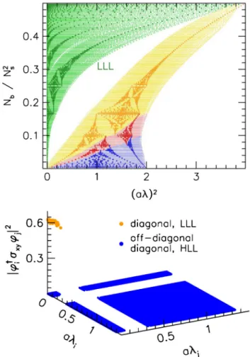
FIG. 3. Top: the spectrum of the two-dimensional staggered Dirac operator in the interacting case—evaluated on one slice of a typical four-dimensional gauge configuration (for details see the text). For comparison, the free-case eigenvalues from Fig.2are also included. Again, the color coding is based on the continuum LL degeneracy as in Fig.2and explained in the text. As it turns out, the LLL eigenvalues are separated from the rest, but HLLs cannot be distinguished in the interacting case. Bottom: the absolute value square of the matrix elements of the relativistic spin operatorσxyin the basis of the two-dimensional eigenmodes.

Notice the separation of the LLL modes from the HLL states by the gap (white region in the bottom plane) and the very different matrix elements ofσxy on the two set of modes.

Q^2D_top¼ 1 2π

Z

d²xF_xy¼ 1

2πL²·qB¼N_b; ð4Þ and the usual four-dimensional notion of handedness is replaced by the spin direction, thus the index theorem entails thatQ^2D_top¼N_↑−N_↓equals the difference of the number of spin-up and spin-down polarized zero modes. In addition, in two dimensions the “vanishing theorem” [39–41]ensures that eitherN_↑orN_↓is zero. Thus, forqB >0the only states in the spectrum with definite spin have spin up and according to Eq.(4)N_b¼N_↑. Indeed, the LLL eigenvalues vanish in the continuum,²and their degeneracy isN_b(for each color).

To demonstrate that even in the presence of color interactions the LLL only accommodates spin-up states, in the lower panel of Fig. 3 we plot the squared matrix elementsjφ^†_iσxyφjj²of the spin operator³σxy¼σz for the down quark at a magnetic flux quantumN_b¼10. Besides the separation of the LLL modes (i≤N_bN_c×2) from the HLL modes (i > N_bN_c×2), the two sets are also clearly distinguished by their spin matrix element. In particular, we find thatσxyis almost perfectly diagonal in the eigenmode basis—the off-diagonal matrix elements are below 10⁻⁴. For the diagonal elements, the HLL entries are also sup- pressed (below 10⁻²), while the LLL entries are much larger, in this case around 0.6. In fact, the spin of the LLL modes approaches unity in the continuum limit. Thus, the classification of the two-dimensional modes based on their mode number (LLL degeneracy) coincides with the clas- sification based on their spin.

It is therefore the index theorem that protects the LLL states from mixing with HLL modes, resulting in the persistence of the gap even in the presence of QCD interactions. To show that the above characteristics remain to hold in the continuum limit, we plot the gap for various lattice spacings in a fixed physical volume L² in the upper panel of Fig.4. The employed QCD configurations are two-dimensional slices of typical high-temperature (T≈400MeV) four-dimensional gauge configurations with aspect ratio N_s=N_t¼4 and N_s¼16…48. The gap is shown this time in physical units: the magnetic flux N_b¼qBL²=ð2πÞ on the horizontal and the eigenvalue in units of the bare quark mass on the vertical axis.⁴ Apparently, the gap edges remain well-defined also in the limita→0(i.e.N_t→∞). To be more specific, in the lower panel of the same figure we plot the widthδλof the

gap as a function of N_b, together with the eigenvalue spacing just above the gap. We see that the gap width always largely exceeds the typical spacing—in other words, the gap at small flux quanta is indeed a well- defined physical structure that survives the continuum limit. Notice moreover that as the continuum limit is approached, the LLL states—while having a fixed multi- plicityN_cN_b—are compressed towards zero, in accordance with their would-be-zero-mode nature.

Moreover, these (near) zero modes are robust with respect to the fermion discretization. We have found the overlap operator to yield the LLL number of zero modes below a gap, too (not shown). Even the Wilson operator, which possesses complex eigenvalues, reproduces these features. Figure 5 shows the spectrum of the Wilson FIG. 4. Top: the gap between the LLL and the HLLs in physical units on two-dimensional slices of full QCD for various lattice spacings (the different eigenvalue sets have been shifted verti- cally for better visibility). Bottom: the width of the gap (solid lines) compared to the typical eigenvalue spacing just above the gap (dotted lines). The color coding of the upper panel matches that of the lower panel.

2In the staggered discretization the LLL modes are not real zero modes but are well separated from the HLL eigenvalues. In the overlap formulation[42,43]these modes become exact zero modes.

3The staggered discretization of the spin operator is detailed in Ref.[27].

4This choice of normalization is dictated by the fact that expressing the eigenvalues in units of the bare quark mass leads to a renormalization-group-invariant spectral density [44], and is thus required to obtain a meaningful continuum limit.

LANDAU LEVELS IN QCD PHYSICAL REVIEW D 96,074506 (2017)

operator on the same background as in Fig.3. Again, (a) a gap in the spectrum is visible and (b) the number of eigenvalues below the gap agrees with the degeneracy of the continuum LLL.⁵This finding confirms once more the power of the index theorem: although it is strictly valid only in the continuum, it governs the low end of (two- dimensional) lattice spectra with magnetic fields.

Finally we remark that above we presented the pronounced features of the spectrum using high-temperature QCD ensembles, but our main conclusions remain unchanged if we use instead gauge configurations in the confined phase.

We like to understand this as follows: Confinement is contained in properties of Polyakov loops, i.e., in temporal links. It is well-known that, on the other hand, the spatial string tension—as a measure for correlations in the spatial links—changes smoothly across the deconfinement transi- tion (see, e.g.,[46]). It is the spatial links in thex-yplane on which the magnetic field acts primarily and from which we measure the two-dimensional spectra. Different temporal links do not modify these effects qualitatively, they“only” change the correlations among differentx-yplanes.

B. Four dimensions

Next, we generalize the concept of Landau levels to four dimensions in Euclidean spacetime, with the magnetic field pointing in the z direction. In the absence of color

interactions, the Dirac equation for thezandtcoordinates decouples from the Landau problem in thex-yplane and has free wave solutions with momenta p_z and p_t. Thus, the eigenmodes factorize asψnαpzpt¼φnα⊗e^ipzz⊗e^iptt, wherenlabels the LL andαthe degenerate modes within each level. The squared eigenvalues and their degeneracies read

λ²npzpt¼qB·2nþp²_zþp²_t; νnpzpt¼2N_b·N_c·ð2−δ_n;0Þ:

ð5Þ (Here we assumed strictly zero temperature, i.e., an infinite size in the temporal direction.) Therefore, each Landau level has become an infinite tower ψ_nαpzpt of states, involving all the allowed momenta in thezandtdirections.

The density of statesρðλÞ—since it is built up by a set of shifted two-dimensional densities—is piecewise linear with jumps at the onsets ffiffiffiffiffiffiffiffiffiffiffi

p2nqB

, as was visualized in the left panel of Fig.1. As a consequence, it is not possible anymore to separate the LLL from the HLLs just by looking at the eigenvalues λnp_zp_t, as we discussed above in Sec.II. Clearly, we need to extract the Landau index n from the eigenmode, or, in other words, work with a projectorPthat projects onto the subspace spanned by the modes with the lowest Landau indexn¼0,

continuum;non-int:∶P¼ X

pz;pt

X

α

ψ0αpzp_tψ^†_0αpzpt

¼X

α

φ_0αφ^†_0α⊗1z⊗1t: ð6Þ On the lattice, the eigenmodes still factorize asψip_zp_t¼ φi⊗ ¹ffiffiffiffi

Ns

p e^ipzz⊗ ¹ffiffiffiffi

Nt

p e^iptt [here i runs over all the two- dimensional modes, see our remark after Eq.(2)]. Instead of using the plane wave basis in thezandtdirections, we can also span the same space by using the coordinate basis consisting of states localized at a single value ofzand oft, ψiztðx; y; z⁰; t⁰Þ ¼φiðx; yÞ⊗δzz⁰ ⊗δtt⁰: ð7Þ After ordering the φi according to their eigenvalues, the first N_cN_b×2 two-dimensional states correspond to the LLL (see Fig.2). Therefore, a valid way to rewrite(6)is to only include these modes,

lattice;non-int:∶ P¼ X

i≤NcNb

X

doublers

X

z;t

ψiztψ^†_izt

¼ X

i≤NcNb

X

doublers

φiφ^†i ⊗1z⊗1t; ð8Þ where the sum over doublers appears due to the twofold doubling of staggered fermions in two dimensions. For a similar definition of the LLL-projector for Wilson quarks in the free case, see Ref.[19].

If QCD interactions are switched on, the components of the four-dimensional Dirac operator D¼D_xyþD_zt in FIG. 5. Spectrum of the two-dimensional Wilson-Dirac oper-

ator with (squared) modulus of the eigenvalues on the horizontal axis. The background configuration and the color coding is the same as in Fig.3. Again, the LLL is separated by a gap in the spectrum and the number of eigenvalues below the gap is consistent with the continuum LLL degeneracy.

5A few remarks are in order here: Since the Wilson-Dirac operator has no doublers unlike the staggered operator, the LLL degeneracy isN_cN_b. The bending of the LLL branch away from aλ¼0 signals additive mass renormalization, see [45]. The closing of the gap at high N_b=N²_s is due to lattice artifacts.

general do not commute, i.e. the eigenmodes do not factorize as in the free case above. Nevertheless, we may still employ the basis of the eigenstates φ^ðz;tÞi of D^ðz;tÞxy for each x-y plane of the lattice, labeled by the coordinatesz,t. The factorized modesψiztare built up from these, similarly as in Eq. (7),

ψiztðx; y; z⁰; t⁰Þ ¼φ^ðz;tÞi ðx; yÞ⊗δzz⁰ ⊗δtt⁰: ð9Þ Thus, the projection in this setting reads

lattice;interacting∶P¼ X

i≤NcN_b

X

doublers

X

z;t

ψiztψ^†_izt: ð10Þ

This is the projector we will use in full four-dimensional QCD to pick out the states corresponding to the LLL. Later we will also use the same construction but composed of the eigenmodesφ~^ðz;tÞ_i of the two-dimensional Dirac operator at vanishing magnetic field. Similarly as above, this uses ψ~iztðx; y; z⁰; t⁰Þ ¼φ~^ðz;tÞi ðx; yÞ⊗δzz⁰ ⊗δtt⁰ and reads

P~ ¼ X

i≤NcNb

X

doublers

X

z;t

ψ~iztψ~^†izt: ð11Þ

Once again, P~ involves the same number N_cN_b×2 of modes as P does, but the modes are eigenstates of the B¼0Dirac operator.

Our numerical results will show that the four-dimensional modes ofDnever correspond purely to the LLL or to a HLL but instead—owing to the mixing between the variousx-y planes via gluon fields in thezandtdirections—have overlap both withPand with its complement1−P. Nevertheless, for typical low-lying four-dimensional modes, there is a distinct jump in the overlap with ψizt betweeni¼N_cN_b×2 and i¼N_cN_b×2þ1i.e. just at the border of the LLL.

This is visualized in the upper panel of Fig. 6 for normalized four-dimensional modesϕfor the down quark (q_d¼−e=3) at T¼400MeV. We define the overlap factor as

W_iðϕÞ ¼ X

doublers

X

z;t

jψ^†_iztϕj²; ð12Þ

where the sum also includes the two two-dimensional doublers and the scalar productψ^†_iztϕinvolves a sum over all lattice points. The completeness of the ψizt modes ensures that the normalization isP

iW_iðϕÞ ¼ϕ^†ϕ¼1. We average over four-dimensional modes in a small spectral interval and over several gauge configurations. The mag- netic flux used here isN_b¼8, leading to a LLL degeneracy of N_cN_b¼24. The upper panel of Fig. 6 reveals that low-lying modesϕ tend to have larger overlap with two- dimensional LLL modes than with HLL states. W_i also remains constant in the LLL region i≤N_bN_c, suggesting

the equivalence of all two-dimensional lowest Landau levels in this respect. This feature, together with the drastic downward jump at the end of the LLL region remains pronounced even in the continuum limit.

In the lower panel of Fig.6 we plot the same quantity, only this timeϕare high-lying four dimensional modes that are expected to have less overlap with the LLL. Indeed, the pronounced downward jump becomes a slight upward jump, so that these modes can be rather thought of as being HLL-dominated. We also mention that the structures visible in Fig. 6 disappear for B¼0 and the overlap becomes a smooth, monotonically decreasing function.

Another important aspect regarding LLL-projected fer- mions is the locality of the fermion action corresponding to the Dirac operator restricted to the LLL subspace. Note that already in the continuum, the lowest Landau level spreads over a rangelB¼1= ffiffiffiffiffiffi

pqB

in the plane perpendicular to the FIG. 6. The overlap(12)of four-dimensional eigenmodes with the two-dimensional modes as a function of the index (in units of N_c¼3) of the latter for a magnetic flux quantumN_b¼8. The upper panel corresponds to low-lying four-dimensional modes (with eigenvalue 220<λ=m <225) while the lower panel represents bulk modes (535<λ=m <545) on configurations generated atT≈400MeV.

LANDAU LEVELS IN QCD PHYSICAL REVIEW D 96,074506 (2017)

magnetic field (see, e.g., Ref. [2]), so that the LLL- projected quark action involves (contrary to usual QCD) the product of quark fields smeared over the range lB. A nontrivial check of our lattice construction is whether this localization range is reproduced. The original Dirac oper- ator without the projection P is ultralocal as it only uses nearest neighbor links. Thus, for LLL-projected fermions we need to check the locality of the projector itself. As can be seen directly from Eqs. (9) and (10), P is ultralocal in thezandtdirections. To discuss locality in thex-yplane,

we consider a source vector ξ localized at the point ðx; y; z; tÞ and the vector ψ ¼Pξ obtained by projecting with P. We measure LðdÞ ¼ h∥ψðx⁰; y⁰; z; tÞ∥i, with d¼ ffiffiffiffiffiffiffiffiffiffiffiffiffiffiffiffiffiffiffiffiffiffiffiffiffiffiffiffiffiffiffiffiffiffiffiffiffiffiffiffi

ðx−x⁰Þ²þ ðy−y⁰Þ²

p the distance from the source

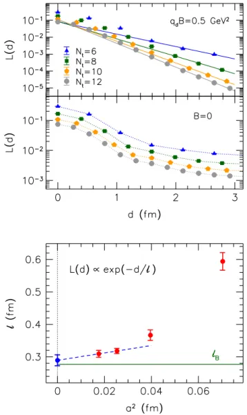
in thex-yplane. As the upper panel of Fig.7reveals, this quantity falls off exponentially with the distance, signaling that interactions between sufficiently separated quark fields are indeed suppressed—once the averaging over gluonic configurations is performed. In the lower panel of Fig.7we perform thea→0 extrapolation of the decay length and find that in the continuum limit it is indeed consistent with the expected value lB≈0.28fm for the magnetic field considered here. We emphasize that the locality ofP(in the sense described above) is a highly nontrivial finding that arises from the interplay of the LLL modes.⁶In general, the projection onto a subset of eigenmodes of the Dirac operator is a highly nonlocal object. We demonstrate this by applying the same construction atB¼0—building the projector P~ of Eq. (11) from the lowest N_bN_c×2 two- dimensional modes at vanishing magnetic field. The so obtained object does not appear to exhibit exponential decay, see the upper panel of Fig.7.

III. OBSERVABLES

Having prescribed the procedure to project an arbitrary four-dimensional mode to the LLL sector, we are in the position to test to what extent certain QCD observables are LLL dominated. We work with three quark flavors indexed byf¼u, d, s. The observables can be derived from the QCD partition function Z, which is written using the Euclidean path integral over gluon A_μ and quark fields Ψ¼ ðψu;ψd;ψsÞ^⊤,

Z ¼ Z

DA_μDΨDΨ¯ e^−SG−SF; ð13Þ S_F ¼Ψ¯MΨ¼ X

f¼u;d;s

¯

ψfM_fψf; ð14Þ

where S_G and S_F are the gluonic and fermionic actions, respectively, and M¼diagðM_u; M_d; M_sÞ with flavor blocks M_f¼D_fþm_f denotes the quark matrix. The Dirac operator is flavor-dependent due to the different electric charges: q_u¼−2q_d¼−2q_s¼2e=3 with e >0 the elementary charge. Integrating out the fermion fields analytically, the expectation values of quark bilinears for the flavorf read

FIG. 7. Top: the expectation valueLðdÞof the modulus of the vector obtained by projecting a localized source on the LLL, as a function of the distancedfrom the source, for a magnetic field q_dB¼0.5GeV². For the proper definition ofLðdÞsee the text.

The exponential decay (solid lines) forB >0in the upper half of the panel demonstrates the locality (in the sense described in the text) of the LLL-projected fermionic action. For theB¼0data shown in the lower half of the panel no such decay is observed.

Bottom: the continuum extrapolation of the decay length based on the two finest lattices, compared to the expected localization lengthlB¼1= ffiffiffiffiffiffiffiffi

q_dB p .

6We mention that the locality of the action inlattice units(i.e., l→0fm for a→0) for usual QCD is a prerequisite for the universality of the continuum limit. For the LLL-projected action the microscopic details of the discretization are damped by the magnetic localization length, present even in the continuum theory. Strictly speaking, the universality argument can therefore only be applied forB→∞wherelB→0.

hψ¯fΓψfi ¼ T 4V

1 Z

Z

DA_μe^−SGdet¹⁼⁴½Mtr½M⁻¹_f Γ: ð15Þ Here, the rooting trick for staggered quarks is employed to reduce the number of flavors to three in the continuum limit and the division by the four-volume V=T renders the observable intensive. The details of our lattice setup, includ- ing the simulation algorithm, the implementation of the magnetic field and the line of constant physics to set the quark massesm_u¼m_d andm_sare described in Refs.[4,47].

To find the LLL contribution to the observable(15), we work with the projector of Eq.(10), which projects onto the subspace spanned by all of the two-dimensional LLL modes (defined on two-dimensional slices corresponding to all values ofzand oft). The projector is a block-diagonal matrix in flavor space, P¼diagðPu; P_d; P_sÞ. The LLL projection amounts essentially to replacing the fermion matrix Mby its projected versionPMP. After integrating out the fermions,Mshows up both in the trace and in the

determinant in Eq.(15). One can then consider the effect of the LLL projection on the valence quarks in the operator in question—represented by the trace—as well as on the sea quarks that characterize the distribution of the gluonic configurations—represented by the determinant. In the present approach, we only insert the projector in the valence sector. The sea contribution is considerably more complicated to implement and we leave it to a forthcoming study.⁷ Similarly, we only insert the magnetic field in the valence Dirac operator and excludeBin the sea sector, i.e., for the generation of the gauge configurations. This implies that valence quarks feel the magnetic field and are projected to the LLL, while virtual sea quarks behave as if they were electrically neutral. We mention that the valence contribu- tion is dominant for, e.g., the quark condensate at low temperatures[48]but not around the QCD transition[49].

This should be kept in mind in the following.

Our definition of the full and the LLL projected quark bilinears (in the valence approximation) thus reads

hψ¯fΓψfi_B¼ T 4V

1 Zð0Þ

Z

DA_μe^−Sgdet¹⁼⁴½Mð0Þtr½M⁻¹f ðBÞΓ;

hψ¯fΓψfi^LLL_B ¼ hψ¯fP_fΓPfψfi_B ¼ T 4V

1 Zð0Þ

Z

DA_μe^−Sgdet¹⁼⁴½Mð0Þtr½M⁻¹_f ðBÞP_fΓPf: ð16Þ The traces are evaluated using noisy estimators ξj. For the LLL projected observable, this amounts to

trðM⁻¹_f P_fΓP_fÞ ¼trðPfM⁻¹_f P_fΓP_fÞ ¼ 1 N_ξ

X^Nξ

j¼1

ξ^†jP_fM⁻¹_f P_fΓP_fξj; ð17Þ

where P_f is taken from Eq. (10)for the flavor f and we used P²_f¼P_f and the cyclicity of the trace. In the following we consider the quark condensate Γ¼1 and the spin polarization Γ¼σxy and refer to these by the superscripts SandT (for scalar and tensor, respectively).

The staggered discretization of the spin operator σxy

involves gauge links lying in thex-yplane and is detailed in Ref. [27].

Besides the representation of the traces using noisy estimators (which we use below to determine the observ- ables), it is instructive to discuss their relation to the overlap W_iðϕkÞ of the four dimensional modes ϕk with the basis modesψiztcarrying the two dimensional indexi, defined in Eq.(12)and visualized in Fig. 6. To see this relation, we use the eigenmode basis of the four-dimensional Dirac operator Dϕk¼iλkϕk. In this representation, the LLL-projected bilinears read

tr½M⁻¹_f ðBÞP_f ¼X

k

m λ²_kðBÞ þm²

X

i≤NcN_b

W_iðϕkÞ;

tr½M⁻¹_f ðBÞPfσxyP_f≃X

k

m λ²_kðBÞ þm²

X

i≤NcNb

X

doublers

X

z;t

jψ^†iztϕkj²· φ^ðz;tÞi

†σ^ðz;tÞxy φ^ðz;tÞi

ψ^†_iztσxyψizt

zfflfflfflfflfflffl}|fflfflfflfflfflffl{

≃X

k

m λ²_kðBÞ þm²

X

i≤NcNb

W_iðϕkÞ·φ^†iσxyφi; ð18Þ

7Here we mention only that if one wants to insertPin the determinant, one should also“quench”the HLL modes, i.e., the correct replacement would beM→PMPþ1−P.

LANDAU LEVELS IN QCD PHYSICAL REVIEW D 96,074506 (2017)

where we used the symmetry of D that its eigenvalues appear in complex conjugate pairs. The spin operatorσxyis diagonal in the zand t coordinates, which allowed us to rewrite the matrix element in the second relation using the two-dimensional modesφiand the blockσ^ðz;tÞxy living on the slice z, t. In the first step of the second relation we used the fact thatσxyis to a good approximation diagonal in the two dimensional modes even in the presence of color interactions, see the lower panel of Fig.3. Moreover, in the second step we approximated the matrix element ofσ^ðz;tÞxy on the two-dimensional modesφ^ðz;tÞ_i to be independent of the coordinatesz,t, which we find to hold if the average over gluon configurations is performed.

In contrast to the LLL-projected observables of Eq.(18), the full observables involve a sum over all values ofi. The upper panel of Fig. 6tells us that the contribution of the overlaps W_i≤NcNbðϕkÞ to the total P

iW_iðϕkÞ is enhanced for low-lying modesϕk. Naively, this works in favor of the LLL dominance of the condensate, however,hψ¯fψfi also contains ultraviolet divergent contributions so that a sen- sible comparison of the LLL-projected and the full observ- ables necessitates renormalization. The situation is similar for the spin polarization. In addition to the overlaps W_i, here the matrix elements φ^†_iσxyφi for i≤N_cN_b are also much larger than for higheri, see the lower panel of Fig.3, which (again, naively) enhances the LLL-dominance for this observable even further. Our next step is therefore the renormalization of both observables, which we discuss in the next subsection.

A. Renormalization

Bothhψ¯fψfi_B andhψ¯fσxyψfi_B contain additive as well as multiplicative divergences. However, it turns out that somewhat different renormalization procedures are required for the condensate and for the spin polarization.

Let us considerhψ¯fψfi_Bfirst. As the analytic calculation in the free case reveals (see Appendix A), the LLL pro- jected and the full condensates contain different divergen- ces (logarithmic for the former and logarithmic plus quadratic divergences in the cutoff for the latter). Thus, simply taking the difference of the two quantities is not sufficient to cancel these terms. Instead, we consider two different routes to deal with these divergences.

First, we use the gradient flow of the gauge fields to make both the LLL projected and the full observables ultraviolet finite. This procedure smears the gluon[50]and the fermion [51] fields over a smearing range R_s and thereby eliminates ultraviolet noise and with that the additive divergent contribution to physical quantities.

The smearing radius is in spirit similar to a momentum cutoffΛ¼1=Rs. We choose the magnetic field to set the smearing range: R_s¼c·ðeBÞ⁻¹⁼² with c≈1 and check that the results depend only mildly onc. Our implementa- tion of the gluonic and fermionic flow for staggered quarks

is detailed in Ref. [52]. The so renormalized observable reads

C^S_f≡hψ¯fψfi^LLL_B ðR_sÞ hψ¯fψfi_BðRsÞ

R_s¼c= ffiffiffiffi

peB: ð19Þ

The second approach does not involve additional ultra- violet cutoffs like the smearing radius above. Instead, the additive divergences are canceled here by taking the difference between the expectation values at B >0 and atB¼0. For the full condensate this is a straightforward procedure that gives the change of the condensate due to the magnetic field,

Δhψ¯fψfi_B¼ hψ¯fψfi_B−hψ¯fψfi_B¼0: ð20Þ For the LLL projected condensate it is somewhat less obvious how to define this difference. The analysis of the free case (see Appendix B) reveals that the divergences can be canceled if one performs a similar projection in the B¼0 term as well, which involves the projector P~ of Eq. (11), built from the eigenmodes of the B¼0 Dirac operator. We then define the subtracted LLL condensate as Δhψ¯fψfi^LLL_B ¼ hψ¯fψfi^LLL_B −hψ¯fP~_fψfi_B¼0: ð21Þ We emphasize that in theB >0term the projector projects on the N_cN_b×2 lowest eigenmodes of the two- dimensional B >0 Dirac operator. In the B¼0 term, P~_fprojects on the same number of modes, but this time of the B¼0 Dirac operator. Using this construction, our second ratio reads⁸

D^S_f≡Δhψ¯fψfi^LLL_B

Δhψ¯fψfi_B : ð22Þ For the spin polarization (superscript T), the ratio C_f can be defined using the same prescription as for the condensate,

C^T_f≡hψ¯fσxyψfi^LLL_B ðRsÞ hψ¯fσxyψfi_BðR_sÞ

Rs¼c= ffiffiffiffi

peB: ð23Þ

The ratioD^T_f must be defined differently, sincehψ¯fσxyψfi_B vanishes identically atB¼0. Namely, in the absence of the magnetic field, there is no preferred direction and the spin polarization averages to zero. However, we can exploit the

8Notice that D^S_f involves the B¼0 projector P, which~ — according to the discussion at the end of Sec.II B—corresponds to a nonlocal operator and might complicate the continuum limit of D^S_f. From this point of view, the first ratio C^S_f is more advantageous. Nevertheless, below in Sec.IVwe will find that bothC^S_f andD^S_f give similar results.

fact that the divergences of the LLL and of the full observable coincide this time. This is supported by the calculation in the free case in AppendixA. This divergent piece, denoted by T^div_f , has been determined⁹ at zero temperature in Ref. [27] using the method summarized in Appendix A. Therefore we have

D^T_f≡hψ¯fσxyψfi^LLL_B −T^div_f

hψ¯fσxyψfi_B−T^div_f : ð24Þ Let us now turn to the multiplicative renormalization.

The renormalization constants are expected to be indepen- dent of the magnetic field, and the LLL-approximation is

assumed to accurately describe strong magnetic fields.

Thus it seems natural to assume that the renormalization constants in the full theory and for the LLL coincide, and ratios of the LLL-projected and the full observables—like C_f andD_f above—are free of multiplicative divergences.

However, since defining the LLL-projection on a finite lattice effectively involves the asymptotic limit B→∞ beforethe continuum limita→0—i.e. with the magnetic field exceeding even the cutoff—the ultraviolet behavior might still be affected. Whether this is the case should be checked in the future. For this reason, in the present paper we do not perform a continuum extrapolation of our results but merely show data obtained using different cutoffs.

IV. RESULTS

We have performed measurements for a range of temper- atures and magnetic fields using four lattice ensembles with N_t¼6, 8, 10, and 12. These serve to approach the continuum limit a→0 at a fixed temperature T owing toT¼1=ðN_taÞ. Thus, the larger N_t, the closer we are to the continuum. The aspect ratios were set toN_s=N_t¼4to keep the physical volume fixed. Throughout the rest of this section we consider the down quark flavorf¼d. Since we FIG. 8. The ratiosC^S_d(left panels) andD^S_d(right panels) for the quark condensate as functions of the magnetic field at a temperature T¼124MeV (upper panels) andT¼170 MeV (lower panels).

9In fact, the determination ofT^div_f in Ref.[27]was carried out with the magnetic field both in the valence and in the sea sector taken into account. This we checked to be a sub-percent effect compared to hψ¯fσxyψfi_B at low temperatures, but becomes increasingly important as T grows and the expectation value reduces. We find that the systematic error in T^div due to neglecting the sea contribution is much smaller than lattice artefacts for our lowest two temperatures T¼124MeV and T¼170MeV so in the following we only consider these simulation points forD^T_f.

LANDAU LEVELS IN QCD PHYSICAL REVIEW D 96,074506 (2017)

only implement the magnetic field and the LLL-projector in the valence sector, for the bilinears for the up quark we identically have hψ¯uΓψui_B ¼ hψ¯dΓψdi_2B (here we also exploited parity symmetry B↔−B).

We begin the presentation of the results with the quark condensate. The two ratiosC^S_dandD^S_dof Eqs.(19)and(22) are plotted in Fig.8for two temperatures, below and above the finite temperature QCD crossover. Both combinations give similar results, rising from about 30% to 60%–80%

within the range 0.4GeV²< eB <1.5GeV². The ratios are expected to approach unity for strong magnetic fields, as the analytic calculation in the free case shows (see Appendix B). In the figures we also include the eB¼3ðπTÞ² vertical line to indicate the point where the magnetic field (times the modulus of the electric charge jq_dj ¼e=3) becomes the largest dimensionful scale in the theory. We measured C^S_d with smearing radii R_s¼1·ðqdBÞ⁻¹⁼²andR_s¼2= ffiffiffi

p3

·ðqdBÞ⁻¹⁼² and found that the systematic effect due to varyingR_sin this range is much smaller than the lattice artefacts.

While for the ratio renormalized through the gradient flow, our N_t¼10 and N_t¼12 results still significantly

differ,D^S_dshows nice scaling towards the continuum limit.

AsBgrows and the magnetic field in lattice units increases, lattice artefacts are expected to become more pronounced, as visible in the right panels of Fig.8. In the following we will take theN_t¼12results forD^S_d as a reference for the validity of the LLL-approximation. The LLL-contribution to this observable reaches 60% at our largest magnetic field and seems to further increase towards unity rather slowly.

This is in agreement with the free case, where the deviation from 1 is of the form1=logðBÞ for largeB, see Eq.(B6).

Next we turn to the spin polarization. The renormalized ratiosC^T_f andD^T_f were defined in Eqs.(23)and(24)above.

We plot both in Fig.9 as functions of the magnetic field for the two temperatures that we considered above. Just as for the condensate, the ratio D^T_d exhibits faster scaling towards the continuum limit. We find thatD^T_d >1i.e., the spin polarization is overestimated by the LLL approxima- tion (for C^T_d this trend is not obvious due to large cutoff effects). This may be understood by noting that σxy is a traceless operator and thatσxyhas matrix elements close to unity on the LLL-modes (see Fig. 3). Thus, the higher modes must have negative matrix elements so that the total FIG. 9. The ratiosC^T_d (left panels) andD^T_d (right panels) for the spin polarization as functions of the magnetic field at a temperature T¼124MeV (upper panels) andT¼170 MeV (lower panels).

trace can vanish and, accordingly, the HLL contribution to

¯

ψσxyψis negative. The deviation ofD^T_d from unity is much milder than for the condensate, remaining below 15% for our finest lattices for the complete range of magnetic fields that we consider here. Notice that the LLL-approximation is expected to work well for this observable since in the free case the HLL-contribution to ψσ¯ xyψ vanishes identically (see Appendix B).

V. SUMMARY

In this paper we investigated the validity of the lowest- Landau-level (LLL) approximation to QCD in the presence of background magnetic fields. In the absence of color interactions, this approximation is based on the structure of the analytically calculable energy levels (the Landau levels) of the quantum system. While the energy of the lowest level is independent ofB, the higher levels have squared energies above B and thus become negligible if the magnetic field is sufficiently strong. Furthermore, the characteristic degeneracy of the Landau levels is proportional to the magnetic flux.

The presence of (nonperturbative) color interactions mixes the levels and therefore complicates this simple picture considerably. In the present paper we demonstrated, for the first time, that the lowest Landau level can nevertheless be defined in a consistent manner even for strongly interacting quarks. The definition of the LLL is based on a two-dimensional topological argument that characterizes the x-y plane (the plane perpendicular to the magnetic field). Namely, the two-dimensional LLL modes have zero energy and their number is a topological invariant fixed by the flux of the magnetic field, independ- ently of the gluonic field configuration. Although these exact zero modes are shifted to nonzero values on a finite lattice, they are still well separated from the rest by a gap in the spectrum. We have shown that this gap is a remnant of the largest gap in the fractal structure usually referred to as Hofstadter’s butterfly in the Hofstadter (lattice) model of solid state physics.

This construction can be performed on eachx-yplane, i.e., for each value of the z and t spacetime-coordinates.

While the two-dimensional modes can be unambiguously classified as belonging or not to the LLL, in four dimensions this is not the case anymore: a general four-dimensional Dirac eigenmode has overlap both in and out of the LLL. We defined the projector Pthat projects the four-dimensional modes onto the subspace of two-dimensional LLL modes for each z and t. Using the projector, we have shown that low-lying four dimensional modes have enhanced overlap with the LLL. For higher four-dimensional modes the overlap with LLL is instead suppressed with respect to HLLs.

Motivated by this, the LLL contribution to standard fermionic observables can be determined. In particular, we concentrated on the quark condensate ψ¯Pψ and the spin

polarizationψ¯PσxyPψ for the down quark. We constructed ratios of the LLL-projected and the full observables that are free of additive divergences (demonstrated in the free case in AppendixA) and that approach unity in theB→∞limit (shown in the free case in AppendixB).

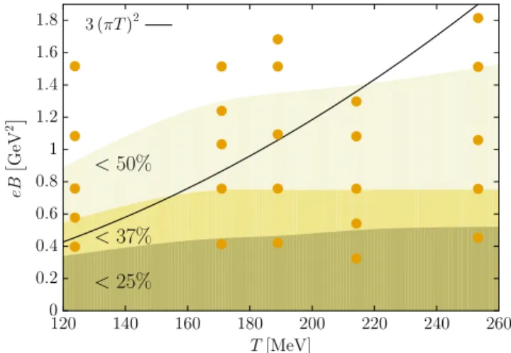
Our results indicate that the LLL approximation under- estimates the quark condensate and overestimates the spin polarization. In addition, the LLL-projected quantities slowly approach the full observables as the magnetic field grows and exceeds further dimensionful scalesΛ²_QCD and ðπTÞ² in the system. Our final results for the condensate (using theN_t¼12data forD^S_d) are visualized for a wide range of temperatures in Fig.10. In this figure the validity of the LLL-approximation is represented in theB-Tplane.

Dark colors stand for regions where the approximation breaks down in the sense that the LLL-projected conden- sate is far away from its full value (so thatD^S_dis less then 25%, 37% or 50%). The white region is where the LLL- contribution to the condensate amounts to more than half of the full condensate. The contours were determined by means of a spline interpolation of D^S_dðBÞ to calculate the magnetic fields where the observable reaches a given percent. Using these threshold magnetic fields for each temperature, a second set of spline interpolations results in continuous T-dependent functions that are shown in the contour plot. The so obtained contours may be compared to the naive expectation q_dB≷ðπTÞ², also indicated in the figure.

Summarizing, we have quantified the systematics of the LLL approximation via first-principle lattice simulations of QCD with background magnetic fields. The results may be compared directly to low-energy models or effective theories employing only the lowest Landau level. We

FIG. 10. Visualization of the validity of the LLL-approximation for the down quark condensate. The lighter the color, the closer the LLL-projected condensate is to the full result. The orange dots denote our simulation points and the solid black line marks q_dB¼ ðπTÞ².

LANDAU LEVELS IN QCD PHYSICAL REVIEW D 96,074506 (2017)