Shared Counters

Lecture 11

Shared Counters

Maybe the most basic operation a computer performs is adding one, i.e., to count. In distributed systems, this can become a non-trivial task. If the events to be counted occur, e.g., at different processors in a multi-core system, deter- mining the total count by querying each processor for its local count is costly.

Hence, in shared memory systems, one may want to maintain a shared counter that permits to determine the count using a single or a few read operations.

11.1 A Simple Shared Counter

If we seek to implement such an object, we need to avoid that increments are

“overwritten,” i.e., two nodes increment the counter, but only one increment is registered. So, the simple approach of using one register and having a node incrementing the counter read the register and write the result plus one to the register is not good enough with atomic read/write registers only. With more powerful registers, things look differently.

Algorithm 25 Shared counter using compare-and-swap, code at node v.

Given: some shared register R, initialized to 0.

Increment:

1: repeat

2: r := R

3: success := compare-and-swap(R, r, r + 1)

4: until success = true Read:

5: return R

11.1.1 Progress Conditions

Basically, this approach ensures that the read-write sequence for incrementing the counter behaves as if we applied mutual exclusion. However, there is a cru- cial difference. Unlike in mutual exclusion, no node obtains a “lock” and needs to release it before other nodes can modify the counter again. The algorithm is lock-free, meaning that it makes progress regardless of the schedule.

143

Definition 11.1 (Lock-Freedom). An operation is lock-free, if whenever any node is executing an operation, some node executing the same operation is guar- anteed to complete it (in a bounded number of steps of the first node). In asyn- chronous systems, this must hold even in (infinite) schedules that are not fair, i.e., if some of the nodes executing the operation may be stalled indefinitely.

Lemma 11.2. The increment operation of Algorithm 25 is lock-free.

Proof. Suppose some node executes the increment code. It obtains some value r from reading the register R. When executing the compare-and-swap, it either increments the counter successfully or the register already contains a different value. In the latter case, some other node must have incremented the counter successfully.

This condition is strong in the sense that the counter will not cease to operate because some nodes crash or are stalled for a long time. Yet, it is pretty weak with respect to read operations: It would admit that a node that just wants to read never completes this operation. However, as the read operations of this algorithm are trivial, they satisfy the strongest possible progress condition.

Definition 11.3 (Wait-Freedom). An operation is wait-free if whenever a node executes an operation, it completes if it is granted a bounded number of steps by the execution. In asynchronous systems, this must hold even in (infinite) schedules that are not fair, i.e., if nodes may be suspended indefinitely.

Remarks:

• Wait-freedom is extremely useful in systems where one cannot guarantee reasonably small response times of other nodes. This is important in multi-core systems, in particular if the system needs to respond to external events with small delay.

• Consequently, wait-freedom is the gold standard in terms of progress. Of course, one cannot always afford gold.

• From the FLP theorem, we know that wait-free consensus is not possible without advanced RMW primitives.

11.1.2 Consistency Conditions

Progress is only a good thing if it goes in the right direction, so we need to figure out the direction we deem right. Even for such a simple thing as a counter, this is not as trivial as it might appear at first glance. If we require that the counter always returns the “true” value when read, i.e., the sum of the local event counts of all nodes, we cannot hope to implement this distributedly in any meaningful fashion: whatever is read at a single location may already be outdated, so we cannot satisfy the “traditional” sequential specification of a counter. Before we proceed to relaxing it, let us first formalize it.

Definition 11.4 (Sequential Object). A sequential object is given by a tuple (S, s

, R, O, t), where

• S is the set of states the object can attain,

11.1. A SIMPLE SHARED COUNTER 145

• s

is its initial state,

• R is the set of values that can be read from the object,

• O is the set of operations that can be performed on the object, and

• t : O × S → S × R is the transition function of the object.

A sequential execution of the object is a sequence of operations o

∈ O and states s

∈ S, where i ∈ N and (s

, r

) = t(o

, s

); operation o

returns value r

∈ R.

Definition 11.5 (Sequential Counter). A counter is the object given by S = N

, s

= 0, R = N

∪ {⊥} , O = { read, increment } , and, for all i ∈ N

, t(read, i) = (i, i) and t(increment, i) = (i + 1, ⊥ ).

We could now “manually” define a distributed variant of a counter that we can implement. Typically, it is better to apply a generic consistency condition.

In order to do this, we first need “something distributed” we can relate the sequential object to.

Definition 11.6 (Implementation) . A (distributed) implementation of a se- quential object is an algorithm

that enables each node to access the object using the operations from O. A node completing an operation obtains a return value from the set of possible return values for that operation.

So far, this does not say anything about whether the returned values make any sense in terms of the behavior of the sequential object; this is addressed by the following definitions.

Definition 11.7 (Precedence). Operation o precedes operation o

if o completes before o

begins.

Definition 11.8 (Linearizability). An execution of an implementation of an object is linearizable, if there is a sequential execution of the object such that

• there is a one-to-one correspondence between the performed operations,

• if o precedes o

in execution of the implementation, the same is true for their counterparts in the sequential execution, and

• the return values of corresponding operations are identical.

An implementation of an object is linearizable if all its executions are lineariz- able.

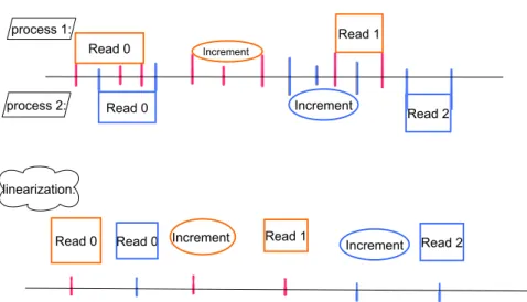
Theorem 11.9. Algorithm 25 is a linearizable counter implementation. Its read operations are wait-free and its increment operations are lock-free.

Proof. All claims but linearizability are easily verified from the definitions and the algorithm. For linearizability, note that read operations are atomic, so we only need to worry about when we let a write operation take place in the linearization. This is easy, too: we choose the point in time when the successful compare-and-swap actually incrementing the value stored by R occurs.

1

Or rather a suite of subroutines that can be called, one for each possible operation.

Figure 11.1: Top: An execution of a distributed counter implementation. Each mark is one atomic step of the respective node. Bottom: A valid linearization of the execution. Note that if the second read of node 1 would have returned 2, it would be ordered behind the increment by node 2. If it had returned 0, the execution would not be linearizable.

Remarks:

• Linearizability is extremely useful. It means that we can treat a (possibly horribly complicated) distributed implementation of an object as if it was accessed atomically.

• This makes linearizability the gold standard in consistency conditions.

Unfortunately, also this gold has its price.

• Put simply, linearizability means “simulating sequential behavior,” but not just any behavior – if some operation completed in the past, it should not have any late side effects.

• There are many equivalent ways of defining linearizability:

– Extend the partial “precedes” order to a total order such that the resulting list of operation/return value pairs is a (correct) sequential execution of the object.

– Assign strictly increasing times to the (atomic) steps of the execution of the implementation. Now each operation is associated with a time interval spanned by its first and last step. Assign to each operation a linearization point from its interval (such that no two linearization points are identical). This induces a total order on the operations.

If this can be done in a way consistent with the specification of the object, the execution is linearizable.

• One can enforce linearizability using mutual exclusion.

11.2. NO CHEAP WAIT-FREE LINEARIZABLE COUNTERS 147

• In the store & collect problem, we required that the “precedes” relation is respected. However, our algorithms/implementations were not lineariz- able. Can you see why?

• Coming up with a linearizable, wait-free, and efficient implementation of an object can be seen as creating a more powerful shared register out of existing ones.

• Shared registers are linearizable implementations of conventional registers.

• There are many weaker consistency conditions. For example one may just ask that the implementation behaves like its sequential counterpart only during times when a single node is accessing it.

11.2 No Cheap Wait-Free Linearizable Counters

There’s a straightforward wait-free, linearizable shared counter using atomic read/write registers only: for each node, there’s a shared register to which it applies increments locally; a read operation consists of reading all n registers and summing up the result.

This clearly is wait-free. To see that it is linearizable, observe that local increments require only a single write operation (as the node knows its local count), making the choice of the linearization point of the operation obvious.

For each read, there must be a point in time between when it started and when it completes at which the sum of all registers equals the result of the read; this is a valid linearization point for the read operation.

Here’s the problem: this seems very inefficient. It requires n − 1 accesses to shared registers just to read the counter, and it also requires n registers. We start with the bad news. Even with the following substantially weaker progress condition, this is optimal.

Definition 11.10 (Solo-Termination). An operation is solo-terminating if it completes in finitely many steps provided that only the calling node takes steps (regardless of what happened before).

Note that wait-freedom implies lock-freedom and that lock-freedom implies solo-termination.

Theorem 11.11. Any linearizable deterministic implementation of a counter that (i) guarantees solo-termination of all operations and (ii) uses only atomic read/write shared registers requires at least n − 1 registers and has step complexity at least n − 1 for read operations.

Proof. We construct a sequence of executions E

= I

W

R

, i ∈ { 0, . . . , n − 1 } , where E

is the concatenation of I

, W

, and R

. In each execution, the nodes are { 1, . . . , n } , and execution E

is going to require i distinct registers; node n is the one reading the counter.

1. In I

, nodes j ∈ { 1, . . . , i } increment the counter (some of these increments

may be incomplete).

2. In W

, nodes j ∈ { 1, . . . , i } each write to a different register R

once and no other steps are taken.

3. In R

, node n reads the registers R

, . . . , R

as part of a (single) read operation on the counter.

As in E

node n accesses n − 1 different registers, this shows the claim.

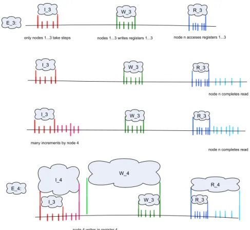
The general idea is to have nodes j ∈ { 1, . . . , i } each perform increments until they finally are forced to write to a new register; we then “freeze” them just before they write to their registers R

. The induction step then argues that

Figure 11.2: Example for the induction step from 3 to 4. Top: Execution E

. Second: We extend E

by letting node n complete its read operation. Third:

We consider the execution where we insert many increment operations by some

unused node between I

and W

. This might change how node n completes its

read operation. However, if node n would not read a register not overwritten

by W

to which the new node writes, the two new executions would be indis-

tinguishable to node n and its read would return a wrong (i.e., not linearizable)

value in at least one of the them. Bottom: We let the new node execute until

it writes the new register first and node n perform its read until it accesses the

register first, yielding E

.

11.2. NO CHEAP WAIT-FREE LINEARIZABLE COUNTERS 149 node i + 1 needs to write to another register than its predecessors if it wants to complete many increments (which wait-freedom enforces) in a way that is not overwritten when we let nodes 1, . . . , i perform their stalled write steps. This is necessary for node n to be able to complete a read operation without waiting for nodes 1, . . . , i; otherwise n wouldn’t be able to distinguish between E

and E

, which require different outputs if i + 1 completed more increments than have been started in E

.

The induction is trivially anchored at i = 0 by defining E

as the empty execution. Now suppose we are given E

for i < n − 1. We claim that node n must access some new register R

before completing a read operation (its single task in all executions we construct).

Assuming otherwise, first consider the following execution. We execute E

and then let node n complete its read operation. As the implementation is solo-terminating, this must happen in finitely many steps of n, and, by lineariz- ability, the read operation must return at most the number k of increments that have been started in E

; otherwise, we reach a contradiction by letting these operations complete (one by one, using solo-termination) and observing that there is no valid linearization.

Now consider the execution in which we run I

, then let some node j ∈ { i+1, . . . , n − 1 } complete k+1 increments running alone (again possible by solo- termination), append W

, and let node n complete its read operation. Observe that the state of all registers R

, . . . , R

before node n takes any steps is the same as after I

W

, as any possible changes by node j were overwritten. Consequently, as n does not access any other registers, it cannot distinguish this execution from the previous run and thus must return a value of at most k. However, this contradicts linearizability of the new execution, in which already k + 1 increments are complete. We conclude that when extending E

by letting node n run alone, n will eventually access some new register R

.

Define R

as the sequence of steps n takes in this setting up to and in- cluding the first access to register R

. W.l.o.g., assume that there exists an extension of I

in which only nodes i + 1, . . . , n − 1 take steps and eventually some j ∈ { i + 1, . . . , n − 1 } writes to R

. Otherwise, R

is never going to be written (by a node different from n) in any of the executions we con- struct, i.e., node n cannot distinguish any of the executions we construct by reading R

; hence it must read another register by repetition of the above argument. Eventually, there must be a register it reads that is written by some node i + 1 ≤ j ≤ n − 1 (if we extend I

such that only node j takes steps), and we can apply the reasoning that follows.

W.l.o.g., assume that j = i+1 (otherwise we just switch the indices of nodes j and i+1 for the purpose of this proof) and denote by I

w

such an extension of I

, where w

is the write of j = i + 1 to R

. Setting W

:= w

W

and E

:= I

W

R

completes the induction and therefore the proof.

Remarks:

• There was some slight cheating, as the above reasoning applies only to un- bounded counters, which we can’t have in practice anyway. Arguing more carefully, one can bound the number of increment operations required in the construction by 2

.

• The technique is far more general:

– It works for many other problems, such as modulo counters, fetch- and-add, or compare-and-swap. In other words, using powerful RMW registers just shifts the problem.

– This can also seen by using reductions. Algorithm 25 shows that compare-and-swap cannot be easy to implement, and load-link/store- conditional can be used in the very same way. A fetch-and-add reg- ister is even better: it trivially implements a wait-free linearizable counter.

– The technique works if one uses historyless objects in the implemen- tation, not just RW registers. An object is historyless, if the resulting state of any operation that is not just a read (i.e., does never affect the state) does not depend on the current state of the object.

– For instance, test-and-set registers are historyless, or even registers that can hold arbitrary values and return their previous state upon being written.

– It also works for resettable consensus objects. These support the operations propose(i), i ∈ N, reset, and read, and are initiated in state ⊥ . A propose(i) operation will result in state i if the object is in state ⊥ and otherwise not affect the state. The reset operation brings the state back to ⊥ . This means that the hardness of the problem is not originating in an inability to solve consensus!

– The space bound also applies to randomized implementations. Basi- cally, the same construction shows that there is a positive probability that node n accesses n − 1 registers, so these registers must exist.

However, one can hope to achieve a small step complexity (in expec- tation or w.h.p.), as the probability that such an execution occurs may be very small.

• By now you might already expect that we’re going to “beat” the lower bound. However, we’re not going to use randomization, but rather exploit another loophole: the lower bound crucially relies on the fact that the counter values can become very large.

11.3 Efficient Linearizable Counter from RW Reg- isters

Before we can construct a linearizable counter, we first need to better understand linearizability.

11.3.1 Linearizability “=” Atomicity

As mentioned earlier, a key feature of linearizability is that we can pretend that linearizable objects are atomic. In fact, this is the reason why it is standard procedure to assume that atomic shared registers are available: one simply uses a linearizable implementation from simpler registers. Let’s make this more clear.

Definition 11.12 (Base objects). The base objects of an implementation of an

object O are all the registers and (implementations of ) objects that nodes may

access when executing any operations of O.

11.3. EFFICIENT LINEARIZABLE COUNTER FROM RW REGISTERS151

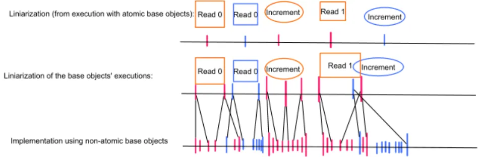
Figure 11.3: Bottom: An execution of an implementation using linearizable base objects. Center: Exploiting linearizability of each base object, we obtain an execution of a corresponding implementation from atomic base objects. Top:

By linearizability of the assumed implementation from atomic base objects, this execution can be linearized, yielding a linearization of the original execution at the bottom.

Lemma 11.13. Suppose some object O has a linearizable implementation us- ing atomic base objects. Then replacing any atomic base object by a linearizable implementation (where each atomic access is replaced by calling the respective operation and waiting for it to complete) results in another linearizable imple- mentation of O.

Proof. Consider an execution E of the constructed implementation of O from linearizable implementations of its base objects. By definition of linearizability, we can map the (sub)executions comprised of the accesses to (base objects of) the implementations of base objects to sequential executions of the base objects that preserve the partial order given by the “precedes” relation.

We claim that doing this for all of the implementations of base objects of O yields a valid execution E

of the given implementation of O from atomic base objects. To see this, observe that the view of a node in (a prefix of) E is given by its initial state and the sequence of return values from its previous calls to the atomic base objects. In E , the node calls an operation once all its preceding calls to operations are complete. As, by definition of linearizability, the respective return values are identical, the claim holds true.

The rest is simple. We apply linearizability to E

, yielding a sequential exe- cution E

of O that preserves the “precedes” relation on E

. Now, if operation o precedes o

in E , the same holds for their counterparts in E

, and consequently for their counterparts in E

; likewise, the return values of corresponding operations match. Hence E

is a valid linearization of E .

Remarks:

• Beware side effects, as they break this reasoning! If a call to an operation affects the state of the node (or anything else) beyond the return value, this can mess things up.

• For instance, one can easily extend this reasoning to randomized imple-

mentations. However, in practical systems, randomness is usually not

“true” randomness, and the resulting dependencies can be. . . interesting.

• Lemma 11.13 permits to abstract away the implementation details of more involved objects, so we can reason hierarchically. This will make our live much, much easier!

• This result is the reason why it is common lingo to use the terms “atomic”

and “linearizable” interchangeably.

• We’re going to exploit this to the extreme now. Recursion time!

11.3.2 Counters from Max Registers

We will construct our shared counter using another, simpler object.

Definition 11.14 (Max Register). A max register is the object given by S = N

, s

= 0 , R = N

∪ {⊥} , O = { read , write (i) | i ∈ N

} , and, for all i, j ∈ N

, t( read , i) = (i, i) and t( write (i), j) = (max { i, j } , ⊥ ) . In words, the register always returns the maximum previously written value on a read.

Max registers are not going to help us, as the lower bound applies when con- structing them. We need a twist, and that’s requiring a bound on the maximum value the counter – and thus the max registers – can attain.

Definition 11.15 (Bounded Max Register). A max register over V ∈ N val- ues is the object given by S = { 0, . . . , V − 1 } , s

= 0, R = S ∪ {⊥} , O = { read, write(i) | i ∈ S } , and, for all i, j ∈ S, t(read, i) = (i, i) and t(write(i), j) = (max { i, j } , ⊥ ).

Definition 11.16 (Bounded Counter). A counter over V ∈ N values is the object given by S = { 0, . . . , V − 1 } , s

= 0, R = S ∪{⊥} , O = { read, increment } , and, for all i ∈ S, t(read, i) = (i, i) and t(increment, i) = (min { i + 1, V − 1 } , ⊥ ).

Before discussing how to implement bounded max registers, let’s see how we obtain an efficient wait-free linearizable bounded counter from them.

Lemma 11.17. Suppose we are given two atomic counters over V values that support k incrementing nodes (i.e., no more than k different nodes have the ability to use the increment operation) and an atomic max register over V values.

Then we can implement a counter over V values and the following properties.

• It supports 2k incrementing nodes.

• It is linearizable.

• All operations are wait-free.

• The step complexity of reads is 1, a read of a max register.

• The step complexity of increments is 4, where only one of the steps is a counter increment.

Proof. Denote the counters by C

and C

and assign k nodes to each of them.

Denote by R the max register. To read the new counter C, one simply reads R.

To increment C, a node increments its assigned counter, reads both counters,

11.3. EFFICIENT LINEARIZABLE COUNTER FROM RW REGISTERS153

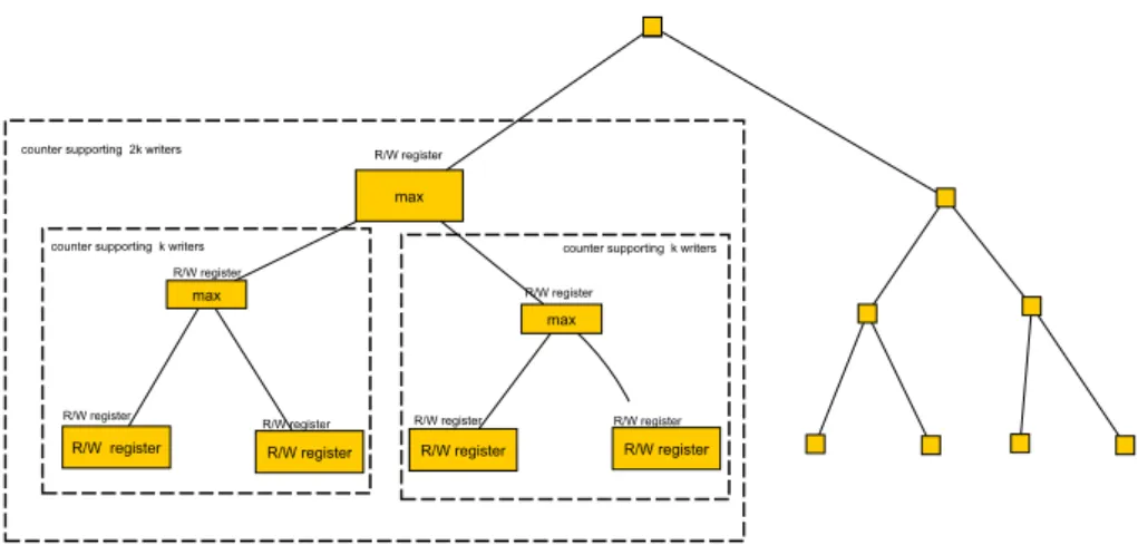
Figure 11.4: The recursive construction from Corollary 11.18, resulting in a tree. The leaves are simple read/write registers, which can be used as atomic counters with a single writer. A subtree of depth d implements a linearizable counter supporting 2

writers, and by Lemma 11.13 it can be treated as atomic.

Using a single additional max register, Lemma 11.19 shows how construct a counter supporting 2

writers using 2 counters supporting 2

writers.

and writes the sum to R. Obviously, we now support 2k incrementing nodes, all operations are wait-free, and their step complexity is as claimed. Hence, it remains to show that the counter is linearizable.

Fix an execution of this implementation of C. We need to construct a corresponding execution of a counter over V values. At each point in time, we rule that the state of C is the state of R.

Thus, we can map the sequence of read operations to the same sequence of read operations; all that remains is to handle increments consistently. Suppose a node applies an increment. Denote by σ the sum of the two counter values right after it incremented its assigned counter. At this point, r < σ, where r denotes the value stored in R, as no node ever writes a value larger than the sum it read from the two counters to R. As the node reads C

and C

after incrementing its assigned counter, it will read a sum of at least σ and subsequently write it to R. We conclude that at some point during the increment operation the node performs on C, R will attain a value of at least σ, while before it was smaller than σ. We map the increment of the node to this step.

To complete the proof, we need to check that the result is a valid lineariza- tion. For each operation o, we have chosen a linearization point l(o) during the part of the execution in which the operation is performed. Thus, if o precedes o

, we trivially have that l(o) < l(o

). As only reads have return values different from ⊥ and clearly their return values match the ones they should have for a max register whose state is given by R, we have indeed constructed a valid linearization.

2

This is a slight abuse of notation, as it means that multiple increments may take effect at

the same instant of time. Formally, this can be handled by splitting them up into individual

increments that happen right after each other.

Corollary 11.18. We can implement a counter over V values and the following properties.

• It is linearizable.

• All operations are wait-free.

• The step complexity of reads is 1.

• The step complexity of each increment operation is 3 d log n e + 1.

• Its base objects are O (n) atomic read/write registers and max registers over V values.

Proof. W.l.o.g., suppose n = 2

for some i ∈ N

. We show the claim by induction on i, where the bound on the step complexity of increments is 3i + 1. For the base case, observe that a linearizable wait-free counter with a single node that may increment it is given by a read/write register that is written by that node only, and it has step complexity 1 for all operations.

Now assume that the claim holds for some i ∈ N

. By the induction hypoth- esis, we have linearizable wait-free counters supporting 2

incrementing nodes (with the “right” step complexities and numbers of registers). If these were atomic, Lemma 11.17 would immediately complete the induction step. Apply- ing Lemma 11.13, it suffices that they are linearizable implementations, i.e., the induction step succeeds.

Remarks:

• This is an application of a reliable recipe: Construct something linearizable out of atomic base objects, “forget” that it’s an implementation, pretend its atomic, rinse and repeat.

• Doing it without Lemma 11.13 would have meant to unroll the argument for the entire tree construction of Corollary 11.18, which would have been cumbersome and error-prone at best.

11.3.3 Max Registers from RW Registers

The construction of max registers over V values from basic RW registers is structurally similar.

Lemma 11.19. Suppose we are given two atomic max registers over V values and an atomic read/write register. Then we can implement a max register over 2V values and the following properties from these.

• It is linearizable.

• All operations are wait-free.

• Each read operation consists of one read of the RW register and reading one of the max registers.

• Each write operation consists of at most one read of the RW register and

writing to one of the max registers.

11.3. EFFICIENT LINEARIZABLE COUNTER FROM RW REGISTERS155 Algorithm 26 Recursive construction of a max register over 2V values from two max registers over V values and a read/write register.

Given: max registers R

and R

over V values, and RW register switch, all initialized to 0.

read

1: if switch = 0 then

2: return R

.read

3: else

4: return V + R

.read

5: end if write(i)

6: if i < V then

7: if switch = 0 then

8: R

.write(i)

9: end if

10: else

11: R

.write(i − V )

12: switch := 1

13: end if

14: return ⊥

The construction is given in Algorithm 26. The proof of linearizability is left for the exercises.

Corollary 11.20. We can implement a max register over V values and the following properties.

• It is linearizable.

• All operations are wait-free.

• The step complexity of all operations is O (log V ).

• Its base objects are O (V ) atomic read/write registers.

Proof sketch. Like in Corollary 11.18, we use Lemmas 11.13 and 11.19 induc- tively, where in each step of the induction the maximum value of the register is doubled. The base case of V = 1 is given by a hard-wired zero: writes do nothing, as they can only write 0; and reads always return 0. More intuitively, the case V = 2 can be seen as the base case, given by a read/write register ini- tialized to 0: writing 0 requires no action, and writing 1 can be safely done, since no other value is ever (explicitly) written to the register; since both reads and writes require at most one step, the implementation is trivially linearizable.

Theorem 11.21. We can implement a counter over V values and the following properties.

• It is linearizable.

• All operations are wait-free.

• The step complexity of reads is O (log V ).

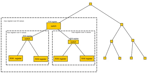
Figure 11.5: The recursive construction from Corollary 11.20, resulting in a tree.

The leaves are empty, which can be used as atomic max registers over 1 value.

A subtree of depth d implements a linearizable max register over 2

values, and by Lemma 11.13 it can be treated as atomic. Using a single read/write register

“switch,” Lemma 11.19 shows how to control access to two max registers over 2

values to construct one that goes over 2

values.

• The step complexity of each increment operation is O (log V log n).

• Its base objects are O (nV ) atomic read/write registers.

Proof. We apply Lemmas 11.13 and 11.18 to the implementations of max reg- isters over V values given by Corollary 11.20. The step complexities follow, as we need to replace each access to a max register by the step complexity of the implementation. Similarly, the total number of registers is the number of read/write registers per max register times the number of used max registers (plus an additive O (n) read/write registers for the counter implementation that gets absorbed in the constants of the O -notation).

Remarks:

• As you will show in the exercises, writing to R

only if switch reads 0 is crucial for linearizability.

• If V is n

, reads and writes have step complexities of O (log n) and O (log

n), respectively, and the total number of registers is n

. As for many algorithms and data structures only polynomially many increments happen, this is a huge improvement compared to the linear step complexity the lower bound seems to imply!

• If one has individual caps c

on the number of increments a node may per- form, one can use respectively smaller registers. This improves the space complexity to O (log n P

i=1

c

), as on each of the d log n e hierarchy levels (read: levels of the tree) of the counter construction, the max registers must be able to hold P

i=1

c

in total, but not individually.

BIBLIOGRAPHY 157

• For instance, if one wants to know the number of nodes participating in some algorithm or subroutine, this becomes O (n log n).

• One can generalize the construction to cap the step complexity at n. How- ever, at this point the space complexity is already exponential.

What to take Home

• This is another example demonstrating how lower bounds do more than just giving us a good feeling about what we’ve done. The lower bound was an essential guideline for the max register and counter constructions, as it told us that the bottleneck was the possibility of a very large number of increments!

• Advanced RMW registers are very powerful. At the same time, this means they are very expensive.

• Understanding and proving consistency for objects that should behave like they are accessed sequentially is challenging. One may speculate that we’re not seeing the additional computational power of multi-processor systems with many cores effectively used in practice, due to the difficulty of developing scalable parallel software.

Bibliographic Notes

This lecture is based largely on two papers: Jayanti et al. [JTT00] proved the lower bounds on the space and step complexity of counters and, as discussed in the remarks, many other shared data structures. The presented counter imple- mentation was developed by Aspnes et al. [AACH12]. In this paper, it is also shown how to use the technique to implement general monotone circuits (i.e., things only “increase,” like for a counter), though the result is not linearizable, but satisfies a weaker consistency condition. Moreover, the authors show that randomized implementations of max registers with maximum value n must have step complexity Ω(log n/ log log n) for read operations, assuming that write op- erations take log

n steps. In this sense their deterministic implementation is almost optimal!

Randomization [AC13] or using (deterministic) linearizable snapshots that support only polynomially many write operations of the underlying data struc- ture [AACHE12] are other ways to circumvent the linear step complexity lower bound. Finally, any implementation of a max register over V values from his- toryless objects requires Ω(min { V, n } ) space [AACHH12].

Bibliography

[AACH12] James Aspnes, Hagit Attiya, and Keren Censor-Hillel. Polyloga-

rithmic concurrent data structures from monotone circuits. Jour-

nal of the ACM, 59(1):2:1–2:24, 2012.

[AACHE12] James Aspnes, Hagit Attiya, Keren Censor-Hillel, and Faith Ellen.

Faster Than Optimal Snapshots (for a While): Preliminary Ver- sion. In Proceedings of the 2012 ACM Symposium on Principles of Distributed Computing, pages 375–384, 2012. Journal preprint at http://cs-www.cs.yale.edu/homes/aspnes/papers/limited-use- snapshots-abstract.html.

[AACHH12] James Aspnes, Hagit Attiya, Keren Censor-Hillel, and Danny Hendler. Lower bounds for restricted-use objects. In Twenty- Fourth ACM Symposium on Parallel Algorithms and Architectures, pages 172–181, 2012.

[AC13] James Aspnes and Keren Censor-Hillel. Atomic Snapshots in O(log

n) Steps Using Randomized Helping. In Distributed Com- puting - 27th International Symposium, DISC 2013, Jerusalem, Israel, October 14-18, 2013. Proceedings, pages 254–268, 2013.

[JTT00] P. Jayanti, K. Tan, and S. Toueg. Time and Space Lower Bounds

for Nonblocking Implementations. SIAM Journal on Computing,

30(2):438–456, 2000.