Dr.JavierRedondo Max-Planck-InstitutfürPhysik,München Prof.Dr.AlejandroIbarra HendrikVogelFebruar2013 Diplomarbeit DarkRadiationfromaHiddenU(1) TechnischeUniversitätMünchenPhysik-Department

(1)

Technische Universit¨at M¨ unchen Physik-Department

Dark Radiation from a Hidden U(1)

Diplomarbeit

von

Hendrik Vogel

Februar 2013

Durchgef¨ uhrt bei

Prof. Dr. Alejandro Ibarra

am

Max-Planck-Institut f¨ ur Physik, M¨ unchen

unter Betreuung von

Dr. Javier Redondo

(2)

ii

(3)

Abstract

We study the contribution of a hidden sector to the effective number of neutrinos Neff during Big Bang nucleosynthesis and the formation of the cosmic microwave background. The hidden sector consists of a massless photon, corresponding to a new U(1) gauge group, and a massive fermion charged under this U(1). Interactions of the hidden sector with the Standard Model particles are mediated via kinetic mixing.

We computeNeff for scenarios where (1) the hidden sector is tightly coupled to the Standard Model particles, and (2) the coupling is very weak and the hidden sector is produced during the evolution of the universe. We extend an existing formalism in the first case and develop a new method in the second case to compute the energy transferred into the hidden sector.

We scan the parameter space to find possible realizations of this model consistent with observations. We point out important parameter regions for further experimental searches in case of a confirmation of an excess in Neff. In the case of a null result, our calculations are useful to constrain models with a minicharged particle and a massless photon.

iii

(4)

Zusammenfassung

Wir untersuchen in dieser Diplomarbeit den Beitrag eines versteckten Sektors zur ef- fektiven NeutrinoanzahlNeff w¨ahrend der Big Bang Nukleosynthese und der Entste- hung des kosmischen Mikrowellenhintergrunds. Der versteckte Sektor besteht aus einem masselosen Photon, welches durch eine zus¨atzliche U(1) Eichgruppe entsteht, und einem massiven Fermion, welches unter dieser neuen U(1) geladen ist. Die Wech- selwirkungen des versteckten Sektors mit den Standardmodellteilchen wird durch kinetisches Mischen erzeugt.

Wir berechnenNeff f¨ur Szenarios, in denen (1) der versteckte Sektor sehr eng an die Standardmodellteilchen gekoppelt ist und (2) die Kopplung sehr schwach ist und der versteckte Sektor w¨ahrend der Evolution des Universums erzeugt wird. Im ersten Fall erweitern wir einen bestehenden Formalismus. Im zweiten Fall entwickeln wir eine neue Methode, um den Energieinhalt des versteckten Sektor zu berechnen.

Wir untersuchen den Parameterraum, um mögliche, mit experimentellen Daten vere- inbare Realisationen dieses Models zu finden. Außerdem nennen wir wichtige Pa- rameterregionen, die für weitere experimentelle Untersuchungen interessant sind, sollte die Existenz eines erhöhten Neff bestätigt werden. Sollte dies widerlegt werden, sind unsere Ergebnisse nützlich, um Modelle mit einem minigeladenen Teilchen und einem masselosen Photon einzuschränken.

iv

(5)

List of Figures

2.1 Relativistic Degrees of Freedom g∗ and Entropy Degrees of Freedom

g∗S . . . 9

2.2 g∗ for Electrons and Positrons . . . 10

3.1 Big Bang Nucleosynthesis . . . 15

3.2 Abundances from BBN . . . 17

3.3 CMB Sky Image . . . 18

3.4 CMB Power Spectrum . . . 20

3.5 Influence of ∆Neff >0 on the CMB spectrum . . . 21

4.1 Rotation Curve of the Galaxy NGC 6503 . . . 24

5.1 Kinetic Mixing Vertices . . . 31

5.2 Hidden Fermion Vertices . . . 32

6.1 Bounds on Minicharged Particles . . . 35

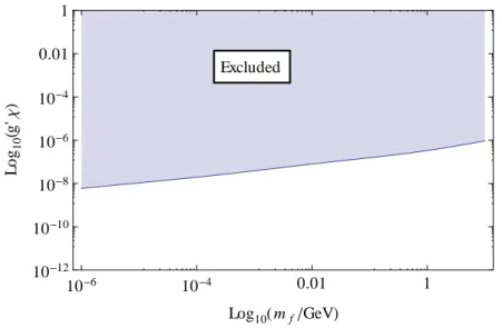
6.2 Exclusion Plot for Minicharged Particles from CMB . . . 37

6.3 Annihilation Diagram . . . 39

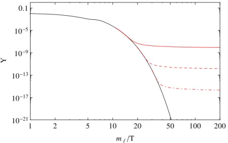
6.4 Examples for the Calculation of Relic Densities . . . 41

6.5 Relic Density of the Hidden Fermion . . . 44

7.1 Comparison of Compton Scattering and Vector Fusion . . . 47

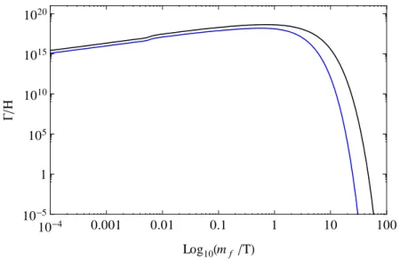
7.2 Γ/H of Compton Scattering γf →γ⁰f . . . 50

7.3 Γ/H of Vector Fusion γγ⁰ →ff¯ . . . 51

7.4 Isotemperature Curves of the Decoupling Temperature T^d . . . 52

7.5 Result forNeff at 3 MeV for a Dark Sector in Equilibrium . . . 53

7.6 Illustration of Important Regions for BBN in Equilibrium . . . 54 viii

(9)

7.7 Result forNeff at CMB for a Dark Sector in Equilibrium . . . 56

7.8 Contribution of Neutrinos and the Hidden Photon toNeff(Equilibrium) 57 7.9 Cuts Through Figure 7.7 . . . 57

7.10 Illustration of Important Regions for CMB in Equilibrium . . . 58

8.1 Illustration of the Sectors . . . 61

8.2 Schematic Illustration of Simulation . . . 61

8.3 Pressure for Different Masses . . . 65

8.4 Energy Transport for e⁺e⁻↔ff¯ . . . 73

8.5 Plasma Frequency . . . 75

8.6 Plasmon Decay . . . 76

8.7 Energy Transport for γf ↔γ⁰f . . . 79

8.8 Result forNeff at BBN (non-equilibrium) . . . 81

8.9 Region A & B for BBN . . . 82

8.10 Region C & D for BBN . . . 82

8.11 Region E & F for BBN . . . 83

8.12 Cuts Through Figure 8.8 . . . 84

8.13 Result for Neff at BBN without Scattering . . . 85

8.14 Result for Neff at CMB (non-equilibrium) . . . 87

8.15 Contribution of Neutrinos and Hidden Photons to the CMB Result forNeff . . . 88

8.16 Region A & B for CMB . . . 88

8.17 Region C & D for CMB . . . 89

8.18 Region E & F for CMB . . . 90

8.19 Region G for CMB . . . 91

8.20 Comparison of Equilibrium and Non-Equilibrium Results for BBN . . 92

8.21 Comparison of Equilibrium and Non-Equilibrium Results for CMB . 93 8.22 Result for Neff at Deuterium Bottleneck . . . 94

8.23 Result for Neff at Deuterium Bottleneck without Scattering . . . 95

ix

(10)

List of Tables

5.1 Summary of the Considered Model . . . 30

8.1 Numerical Test of the Initial Conditions . . . 63

8.2 Initial Conditions for the Dark Sector . . . 63

8.3 Particles Considered in Our Simulation . . . 74

8.4 Parameters Chosen for Plasmon Decay . . . 76

8.5 Goodness of Scaling for Compton Scattering . . . 78

8.6 Parameter Regions for Scattering . . . 79

x

(11)

xi

(12)

Chapter 1 Introduction

Our understanding of the fundamental constituents of nature is incomplete. Al- though our currently best model, the Standard Model of particle physics (SM) [1–3], describes most high-energy phenomena with remarkable accuracy, the SM fails to explain apparent physical phenomena like gravity or dark matter (DM). Especially, the need for DM in cosmology and its easiest theoretical explanation in terms of a particle call for an extension of the SM [4, 5].

Many well motivated models incorporate DM (see [4, 5] and references therein) and the theoretical nature of DM is well understood. Moreover, a variety of complementary experiments exist, ranging from collider searches [6,7] over direct detection measurements (e.g. [8–10]) to indirect searches (e.g. [11,12]). So far, no reproducible DM signal has been measured, and none of the theoretical models have been proven to be realized in nature.

Cosmological observations point towards even more physics beyond the SM, besides DM. Satellites and telescopes, like the Wilkinson Microwave Anisotropy Probe (WMAP) [13], the South Pole Telescope (SPT) [14], and the Atacama Cosmology Telescope (ACT) [15], measure the anisotropy spectrum of the cosmic microwave background (CMB) with great accuracy. They find that our models of the early universe fit the CMB spectrum to a higher precision, if they include some new relativistic particles with very weak interactions [16–18].

The CMB spectrum is not the only cosmological observation hinting at new physics.

In fact, the theoretical predictions of Big Bang nucleosynthesis (BBN) fit observations of the abundances of light elements in the universe more accurately if additional particles are added [19]. Again these particles should be relativistic during BBN and hardly interact with the SM particles and nuclei. This additional component of the universe has been dubbed dark radiation (DR) due to its relativistic nature and since its interactions must be so weak. It is intriguing to develop predictive models incorporating DR to simultaneously improve our predictions for BBN and CMB.

The existence of DR is not fully established since the uncertainties on the measure- 1

(13)

2

ments by WMAP, SPT and ACT are large. Their results are still consistent with an SM cosmology at the 95% confidence level (CL) [16–18]. This also holds for the comparison of the abundances of light elements and the theoretical predictions of BBN [19]. Nevertheless, the fact that a number of experiments independently favor DR makes it worth studying what extensions of the SM could explain these observations. Additionally, the data of the Planck satellite will be published soon [20].

The Planck collaboration is expected to give results for DR with an unprecedented accuracy [21]. With their data, we might be able to confirm the existence of DR.

With BBN and CMB measurements, we can also quantify the amount of DR. Since the effect of DR on BBN and the CMB is equivalent to the effect of neutrinos, it is common to express the amount of DR in terms of its equivalent of SM neutrinos Neff. Neff is also called the effective number of neutrinos.

If DR exists, it should be consistently embedded into an extension of the SM. Pos- sible extensions that explain DR include, e.g., sterile neutrinos [22] and axions [23].

This thesis looks at the implications for DR of a minimal hidden sector extending the SM. This sector is called hidden because the interactions between the hidden sector and the SM particles are very weak. We will frequently call this hidden sector a dark sector (DS).

The DS is realized by adding another local U(1)h group to the SM gauge groups, SU(3)c×SU(2)L×U(1)Y, and introducing particles charged under this U(1)h. Fol- lowing the spirit of a hidden sector, the SM particles are not charged under this U(1)h. Such an additional gauge group is a common feature of extensions of the SM like string theory (e.g. [24]).

The field content of our DS is minimal. The local U(1)h generically introduces a hidden photon (HP) into the theory. We keep the U(1)h unbroken so that the HP is massless. The HP mixes with the SM photon throughkinetic mixing. For a massless hidden photon, this kinetic mixing can be rotated away so that the HP decouples completely from the SM [26]. This fact leads some authors to break U(1)h to obtain a massive HP [26]. In this work, we follow a different approach. We add to the theory a dirac fermion, a hidden fermion (HF), which is only charged under the U(1)h and has strong gauge interactions with the hidden photon. After the kinetic mixing is rotated away, the hidden fermion obtains a small electric charge. It is then called aminicharged particle [26, 27].

Since the hidden photon is always relativistic and does not have tree-level interactions with the SM particles, it is an ideal candidate for DR. The hidden fermion is taken to be massive. Depending on its mass, it either contributes to Neff or the amount of DM in the universe. Its most important role, however, is to act as a bridge between the SM and the DS since it interacts with both, photons and HPs.

It can, therefore, transport energy from one sector to another.

The goal of this work is to find realizations of this dark sector model, in which we are able to obtain the amount of dark radiation favored by BBN and CMB observa-

(14)

3

tions. For this, we study the thermalization of the DS in the early universe. If the coupling is very large, this problem can be solved by applying entropy conservation at decoupling. If the sectors couple very weakly, we need a full calculation solving Boltzmann equations. For the first case, we extend the current formalism. For the second case, we develop a new method to compute the amount of DR.

We also look at constraints that arise due to the minicharge of the hidden fermion.

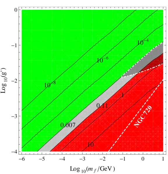
Sub-MeV minicharged fermions are experimentally heavily constrained. For higher masses (MeV-GeV) constraints come from the fact that the HFs form a charged component of DM. We point out the parameter space where HFs are excluded, and where they could be detected in the future. We then indicate parameter regions that are worth exploring in case of a positive result for Neff of the Planck collaboration.

Even if the Planck collaboration should not find any evidence for DR, our results are still useful to constrain hidden particles in this minimal scenario.

The structure of this thesis is the following: In chapter 2 we introduce basic notions of cosmology and introduce the definition of the quantity Neff. In chapter 3 we explain the hints for DR in more detail. Chapter 4 introduces the concept of DM and the calculation of relic densities. We define our model in chapter 5. Constraints on minicharged particles are the topic of chapter 6. In chapter 7, we present our results for the scenario where the DS is coupled strongly to the SM sector. The results for the scenario with weaker couplings are shown in chapter 8. Chapter 9 contains an outlook. We conclude in chapter 10.

(15)

Chapter 2 Cosmology

Cosmology is the study of the origin, structure and expansion of the universe. It includes the investigation of the large-scale structure of the universe, the origin of the elements during BBN, and the CMB.

The simplest model accurately describing our knowledge of the evolution of the universe is the ΛCDM model, in which Λ denotes a cosmological constant and CDM stands for cold dark matter. This model is often referred to as the standard model of cosmology. It assumes that the universe originated from the Big Bang, a very hot and dense initial condition, and expanded according to the laws of general relativity.

Expansion caused the universe to cool down, allowing light elements to form in BBN.

When the temperature fell to 0.26 eV [28], photons decoupled from electrons and nuclei, and the radiation we see today as the CMB was released. Small density fluctuations that were present in the universe acted as seeds to structure formation;

galaxies formed in overdense regions and voids developed in underdense regions.

Today the universe is expanding at an accelerated rate due to the cosmological constant Λ [16].

The most defining features of our universe are that it appears to be homogenous and isotropic [29]. Moreover, it has been expanding for a long time, as observed by [30]. The metric that describes our universe should, therefore, incorporate this homogeneity, isotropy, and expansion.

These three properties can be conveniently described in the Friedmann-Lemaˆıtre- Robertson-Walker metric (FLRW metric):

ds² = dt²−a(t)²

dr²

1−kr² +r²dθ²+r²sin²(θ) dφ²

, (2.1)

where t denotes physical time, a(t) is the scaling factor, r, θ, and φ are comoving spatial coordinates,k is the curvature constant, and we use natural units c=~= 1.

The coordinates r, θ, and φ are called comoving because the expansion of the universe has been factored out into the scaling factor a(t). Comoving distances do

4

(16)

CHAPTER 2. COSMOLOGY 5

not change when the universe expands. Physical coordinates X are obtained by multiplying the comoving coordinates by the scale factor, X(t) = a(t)r. When the universe expands, the scale factor increases. The concept of homogeneity and isotropy are incorporated by making a(t) a function of time only.

The curvature constantk describes the spatial curvature of the metric. By rescaling r, we can normalize it to +1,−1, or 0, corresponding to positive, negative, and zero spatial curvature. In the following, we always setk= 0, which means a flat universe in agreement with experimental observations [16].

The FLRW metric is often cast into a form where the scale factor multiplies the whole metric

ds² =a²(η) dη²−dr²−r²dθ²−r²sin²(θ) dφ²

. (2.2)

In this formula, η is conformal time, defined as dη = dt/a(t). The metric now resembles the Minkowski metric times a conformal scale factor.

One consequence of the expansion of the universe is the redshift of the wavelength of photons. The wavelength λ stretches due to the expansion of space itself [29].

The cosmological redshift z is defined as 1 +z = λ0

λ1

= a(t0)

a(t1). (2.3)

The subscript 0 denotes present values, and the subscript 1 denotes values at some earlier time. One can show [29] that the four momenta p^µ of relativistic particles scale like a⁻¹ and, therefore, decrease with the expansion of the universe.

2.1 The Friedmann Equations

The dynamics of the expansion are governed by Einstein’s equations Rµν −1

2gµνR= 8πGNTµν+ Λgµν. (2.4) Here Rµν is the Ricci curvature tensor, R the scalar curvature, GN = 6.72 × 10⁻³⁹GeV² Newton’s gravitational constant, Tµν the stress-energy tensor, and we have adopted the sign conventions of [29]. In the following, we ignore a cosmological constant since we are mainly looking at epochs in which it is subdominant.

For an isotropic and homogeneous universe, the simplest form of the stress-energy tensor is that of a perfect fluid,

T^µ_ν = diag(ρ,−P,−P,−P), (2.5) where ρ is the energy density, and P is the pressure.

(17)

6 2.1. THE FRIEDMANN EQUATIONS

In the FLRW metric, energy conservation (T^µν_;ν = 0) then leads to a useful equation governing the evolution of ρ:

˙

ρ=−3H(ρ+P), (2.6)

where the dot denotes the time derivative d/dt, and H is the Hubble parameter, defined as

H ≡ a˙

a. (2.7)

From the Einstein equation, one can derive a relation betweenH and ρ, H² =

a˙ a

2

= 8πGN

3 ρ. (2.8)

The universe expands faster when its energy density is larger. Equations (2.6) and (2.8) are two of three equations known as the Friedmann equations. The present value of the Hubble parameter is H0 = 73.8±2.4 km s⁻¹Mpc⁻¹ [31] from measurements of supernovae. The prediction from nine years of WMAP alone is smaller H0 = 70.0 ±2.2 km s⁻¹Mpc⁻¹ [16] but compatible with the former. H0 is often parametrized as H0 = 100hkm s⁻¹ Mpc⁻¹, whereh is the scale factor for the Hub- ble expansion rate.

To solve the Friedmann equations, we must express P as a function of ρ. This equation of state is generally formulated as

P =ωρ, (2.9)

where ω is a proportionality constant. We can solve equation (2.6) for the energy density ρ using equation (2.9). This gives the relation ρ ∝ a^−3(1+ω). Spatial expansion leads to a scaling of space proportional toa³. The energy density of non- relativistic matter, therefore, scales like a⁻³ (ω = 0 ⇒ P = 0). Using ρ∝ a^−3(1+ω) and equation (2.8), one obtains a(t)∝t^2/3 and H = 2/(3t). The Hubble parameter thus decreases with time, i.e., the expansion slows down.

For relativistic particles (radiation), we can neglect masses in computing the energy density. Radiation then scales like ∝ a⁻⁴ (ω = ¹₃ ⇒ P = ¹₃ρ) because, in addition to the volume, the energy decreases as a⁻¹. So, the energy in radiation is redshifted faster than that in matter. For the proportionality of the scale factor a with time, one obtains a∝t^1/2, and the Hubble parameter during radiation domination (RD) scales asH = 1/(2t).

In standard cosmology, the different scaling behavior of matter and radiation divides the history of the universe into two epochs. In the first epoch, that of radiation domination, most of the energy was stored in relativistic particles. The energy density of radiation eventually depletes so much that the energy in matter becomes more important. This epoch is known as matter domination (MD).

(18)

At present, we are in a period where the energy content of the universe is dominated by a cosmological constant with an equation of state compatible with ω =−1 [16].

Since BBN occured during RD, and since the formation of the CMB is notably influenced by DM and DR originating from RD, we focus on RD in this work.

2.2 Thermodynamics of the Early Universe

In the ΛCDM model, after the Big Bang, the universe was initially very hot and dense. For high temperatures, all SM particles were present in the plasma, and their interactions were strong enough to keep them in equilibrium.

Every particle species is described by its phase-space distribution function f(~p, t).

In an isotropic and homogeneous universe, f only depends on the magnitude of the momentum |~p|. In equilibrium, the distribution function is

f(E, t) = 1

exp[(E −µ)/T]±1, (2.10)

whereE =p

|p|²+m² is the energy of the particle andmits mass. The plus sign in the denominator is for the Fermi-Dirac distribution of fermions and the minus sign for the Bose-Einstein distribution of bosons. Chemical potentials µ are extremely small and negligible for our purposes. Consequently, the distribution function for particles and antiparticles are equal. If the particle species is in equilibrium with itself, T denotes the temperature of the particle species. It can happen that this temperature differs from the temperature of the photons if the interactions with the electromagnetic sector become too small. This is the fate of the neutrinos, which decouple from the plasma at T ∼2 MeV.

For largeE/T, the distribution function (2.10) can be approximated by a Boltzmann distribution

f(E, t) = exp

−E T

. (2.11)

This approximation will be used very frequently in the following chapters since it usually changes thermally averaged quantities only by a few percent.

One calculates the number densityn of a particle species in a nondegenerate plasma by integrating over phase space,

n=g

Z d³p

(2π)³ f(~p). (2.12)

Here g is the number of internal degrees of freedom. We calculate g by adding up all combinations of spin states, color degrees of freedom, etc. Hence, for an electron, g = 2; for a massive Z boson, g = 3; and for a quark,g = 6.

(19)

8 2.2. THERMODYNAMICS OF THE EARLY UNIVERSE

Similarly, we calculate the energy density of a particle species by weighting the distribution function with its energy

ρ=g

Z d³p

(2π)³ E(~p)f(~p). (2.13) We can also compute the pressure

P =g

Z d³p (2π)³

|~p|²

3E(~p)f(~p). (2.14)

For relativistic particles, this formula reproduces the equation of state for radiation P = ¹₃ρ. In this limit, ρ and n take the forms [29]

n =gζ(3)

π² T³ and (2.15a)

ρ=gπ²

30T⁴ (2.15b)

for bosons, and

n=g3 4

ζ(3)

π² T³ and (2.16a)

ρ=g7 8

π²

30T⁴ (2.16b)

for fermions. Here ζ(3)≈1.202 is the Riemann zeta function.

We can express the equation for the energy density (2.13) in terms of the energy, ρ= g

2π² Z ∞

m

dE E² (E²−m²)¹²

exp(E/T)±1. (2.17)

Factorizing outT, and introducing new variablesy=E/T andx=m/T, we rewrite this equation as

ρ=T⁴ g 2π²

Z ∞ x

dy y² [y²−x²]¹²

exp(y)±1. (2.18)

For non-relativistic particles, we must account for masses so that the energy and number densities are

ρ≈mn, and (2.19a)

n ≈g mT

2π ³₂

exp

−m T

. (2.19b)

(20)

-5 -4 -3 -2 -1 0 1 2 2

5 10 20 50 100

Log₁₀HTGeVL

g*

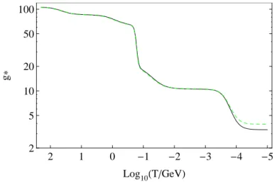
Figure 2.1: Relativistic degrees of freedom g∗ (black) and entropy degrees of freedom g∗S

(dashed green) as a function of the temperature of the universeT. For the fit see appendix A of [32].

The early universe was a plasma of many different particle species with possibly different temperatures. To express the total energy density in terms of one temperature, that of the photons Tγ, it is convenient to introduce a counter for the relativistic degrees of freedom g∗,

g∗ = X

i=bosons

gi

Ti

T 4

+7 8

X

i=fermions

gi

Ti

T 4

. (2.20)

The factor 7/8 corrects for the different statistics of bosons and fermions. The ratios (Ti/T)⁴ accounts for the case when some particles have decoupled from the rest and maintain their own temperature Ti.

We can express the energy density of radiation as ρR = π²

30g∗T⁴. (2.21)

We can now write the Hubble parameter in equation (2.8) as a function of the temperature

H =

r8π³GN

90 g∗¹²T² ≈1.66g∗¹²

T² mP

, (2.22)

wheremP= 1/√

GN≈1.22×10¹⁹GeV is the Planck mass. Hence, the Hubble rate during RD scales as T² if g∗ is constant.

Figure 2.1 shows the evolution of g∗ during RD. Its form has been taken from appendix A of [32]. For highT, all the SM particles are in equilibrium with each other and are relativistic. As the universe expands, it cools down. When the temperature T falls below the mass threshold of a particle species, it is statistically disfavored to

(21)

-3 -2

-1 0

1 2

3 0.0 0.5 1.0 1.5 2.0 2.5 3.0 3.5

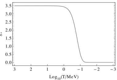
Lo g₁₀HTMeVL g*

Figure 2.2: Contribution of electrons and positrons to the relativistic degrees of freedom g∗ as a function of the temperature of the universe T.

still populate these high mass states. This leads to a reorganization of these states into statistically less suppressed states of lower energy, i.e. the particle species anni- hilates or decays into lighter particles thereby practically vanishing from the plasma.

It can be seen from (2.19) that the suppression of abundances is exponential.

When particles annihilate, they transfers their energy into the rest of the plasma.

When this happens, the universe cools down slower than if g∗ is constant. Usually, the temperature scales as a⁻¹ but during these annihilation the scaling is altered.

Figure 2.2 shows the isolatedg∗ ofe⁺e⁻. The maximum lies at 4(7/8) = 3.5. As the temperature approaches the mass of the electron (511 keV) the curve goes smoothly down to zero.

In figure 2.1, important transitions include the QCD phase transition at around 180 MeV and the e⁺e⁻ → γγ annihilation at around 500 keV due to particles becoming non-relativistic. At the QCD phase transition, the gluons, up- and down quarks are confined into mesons and baryons. By this, the relativistic degrees of freedom g∗ drop by approximately 40 (16 gluonic and 24 quark degrees).

In local thermodynamical equilibrium, entropy is conserved. This also holds when a particle species becomes non-relativistic [29]. The entropy density of the universe s is defined as

s≡ S

V = ρ+P

T , (2.23)

where S is the entropy, and V is a volume element.

With equations (2.13) and (2.14) we can express this as s= 2π²

45 g∗ST³, (2.24)

(22)

where the contribution of non-relativistic particles has been neglected andg∗S is the number of the entropy degrees of freedom, which is defined similar to g∗,

g∗S = X

i=bosons

gi

Ti

T 3

+ 7 8

X

i=fermions

gi

Ti

T 3

. (2.25)

The evolution of g∗S with the expansion of the universe can be seen in figure 2.1.

Conservation of entropy implies that the entropy density fulfills

sa³ = const., (2.26)

so the temperature scales like

a g^1/3_∗S T = const. (2.27)

Entropy conservation plays a very important role to predict how the temperature of a thermalized sector behaves with the scale factor. Moreover, it enables us to compute temperature ratios, after two sectors decoupled from each other. In the SM universe such a decoupling happened for example for the three neutrino species.

After their decoupling, the neutrino energy density scaled like a⁻⁴ due to redshift;

the energy density of the electromagnetic sector did not scale like a⁻⁴ when e⁺e⁻ annihilated. By imposing entropy conservation, we can calculate the temperature ratio Tν/Tγ. One obtains [29]

Tν

Tγ

=

g∗Sν(T^d) g∗Sν

g∗Sγ

g∗Sγ(T^d) ^1/3

=

1× 2

2 + 3.5 1/3

= 4

11 1/3

, (2.28)

whereT^dis the decoupling temperature of the neutrinos. Competing with cosmological redshift parametrized throughH, this decoupling happens when the interaction rate Γ stops being fast enough to maintain the equilibrium distribution of the neutrinos with the rest of the plasma. The approximate temperature of decoupling T^d can be found by solving for T^d in

Γ(T^d)

H(T^d) = 1, (2.29)

where Γ = hσvin is the interaction rate, in which v is the relative velocity of the interacting particles and σ is the cross section; the brackets h i denote the thermal average (see section 4.3),ndenotes the number density of the particle species interacting with the neutrinos. Γ is defined in a similar way for other particles.

Thus, entropy conservation is a convenient way to calculate temperature ratios of two decoupled sectors once T^d has been obtained. For an extension of (2.28) for additional degrees of freedom see [33]. A more general formula for the case of a third sector coupling to the photon will be introduced in chapter 7.3.

(23)

2.2.1 Effective Neutrino Degrees of Freedom N

eff

Additional relativistic particles, like the hidden photon considered in this work, can significantly contribute to the energy density of the universe. This increase in H leads to a faster expansion of the universe. The contribution toH can be significant if the energy density in the dark sector is of the same order as the SM energy density.

Interestingly, such a contribution would influence cosmological observables like the amount of helium ⁴He and deuterium D from BBN. Put in a different way, we are able to predict the existence of additional particles. In chapter 3, we will explain why such a component is favored by BBN.

Complementary to BBN, we can fit the measured CMB spectrum in a better way, if we add additional particles contributing to the energy density of radiation. These particles are not allowed to interact with photons too strongly. Since both results can be explained in terms of the same framework, it is useful to look for extra radiation during both BBN and the formation of the CMB. As the coupling of this extra radiation cannot be too strong, it is often called dark radiation.

We would expect such DR to behave in a similar way as neutrinos. Neutrinos are relativistic during all primordial phases of the universe. They also decouple before BBN and form some interactionless radiation themselves. Unfortunately, the neutrino background is out of our reach by direct detection [34], so we cannot measure its energy content as we can do with the CMB photons. However, the energy density of radiation contributes to the expansion of the universe and controls many dynamical processes in the early universe (BBN and CMB). This makes it possible to measure the total energy of radiation. It is useful to parametrize the amount of radiation in terms of an effective number of neutrinos Neff

ρR = π² 30

"

g∗p+ 27 8Neff

Tν

Tγ

4#

T_γ⁴, (2.30)

where g∗p denotes all relativistic degrees of freedom in thermal equilibrium with photons and the quantity Neff contains all other particles. It contains the SM neutrinos, but can also include contributions from any relativistic particle beyond the SM.Tν/Tγis set to one beforee⁺e⁻ annihilation and to 4/11 aftere⁺e⁻annihilation (see (2.28)). Using only the field content of the SM and assuming instant neutrino decoupling, the value for Neff is

Neff = 3 (ΛCDM). (2.31)

A slightly higher amount of Neff = 3.04 is found if a small heat transfer after the decoupling of the neutrinos is included [35]. Note that although we call Neff

a number, it is generally non-integer. It represents the amount of energy density decoupled from photons. It is just normalized in an illustrative way.

(24)

If we express the energy density of one neutrino species as ρ1ν, equation (2.30) is equivalent to

Neff= ρ3ν +ρDR

ρ1ν

=Nν +NDR, (2.32)

where ρ3ν is the energy density of all SM neutrinos and ρDR is the energy of any dark radiation from an extension of the SM, Nν is the neutrino contribution to Neff

and NDR is the contribution of the DR to Neff.

If the extra radiation decouples from the plasma before neutrino decoupling,Nν = 3 still holds, and it is useful to define ∆Neff as

∆Neff = ρDR

ρ1ν ∝ TDR

Tν

4

, (2.33)

whereTDR is the temperature of the DR andTν is the temperature of the neutrinos.

This can be expressed in terms of the measurable photon energy density

∆Neff =τ8 7

ρDR π²

30T_γ⁴ ∝τ TDR

Tγ

4

, (2.34)

where τ = 1 before e⁺e⁻ annihilation and τ = (11/4)^4/3 after e⁺e⁻ annihilation.

The crucial aspect of this equation is the proportionality∝(TDR/Tγ)⁴. For a sizable

∆Neff, TDR has to be of the order of Tγ. Otherwise, the exponent suppresses ∆Neff

so much that the contribution to DR becomes negligible.

If extra radiation decouples form the plasma after neutrino decoupling. Nν = 3 must not hold anymore if the standard temperature ratioTν/Tγ = 4/11 is changed.

In this case it only makes sense to quote the total Neff. For a formula for Neff with a sector decoupling after e⁺e⁻ annihilation see [33] or section 7.3. One finds that in this scenario, the temperature ratios Tν/Tγ and TDR/Tγ are crucial.

(25)

Chapter 3 Dark Radiation

The ΛCDM model can be tested by looking at the universe as it appears today. Many very precise predictions come from BBN and the CMB spectrum. BBN explains the abundances of light elements. This mechanism will be introduced in section 3.1. The CMB anisotropy spectrum is probably the most accurate way to test the ΛCDM model and can be used to constrain a plethora of cosmological parameters. It will be introduced in section 3.3.

The physics of BBN and the CMB are altered if one changes the particle content of the cosmological theory. A very important example is that extra relativistic particles enhance the expansion rate of the universe with respect to ΛCDM. Indeed, this additional component, dark radiation, is favored by experiments as we will discuss in section 3.4. How the BBN predictions are changed by introducing more relativistic particles is explained in section 3.2. The influence of enhanced expansion on the CMB today is explained in section 3.4.

3.1 Standard BBN

During BBN, the primordial light elements are formed. Figure 3.1 presents the evolution of different elements during this epoch.

The initial abundance of protons and neutrons is crucial as they eventually form all the elements. Protons and neutrons originate during the QCD phase transition. Thereafter, they are kept in thermal equilibrium through the weak interaction reactions

p+e⁻ ↔n+νe,

p+ ¯νe ↔n+e⁺. (3.1)

The mass difference of neutrons and protons is Q= 1.293 MeV. A difference in the abundances of these particles can only arise as soon as the temperature T of the

14

(26)

CHAPTER 3. DARK RADIATION 15

p n

2H

3H

3He

4He

7Li

7Be

1 10 100 1000 10⁴

10^-12 10^-10 10^-8 10^-6 10^-4 0.01 1

0.01 0.03

0.1 0.3

1.

10^-12 10^-10 10^-8 10^-6 10^-4 0.01 1

time@sD

Yields

Temperature@MeVD

Figure 3.1: Evolution of the primordial abundances of elements. Plot by Cadamuro [36]

made with PArthENoPE [37]. The baryon-to-photon ratio is set toη= 6.23×10⁻¹⁰ and the effective neutrino degrees of freedom N_eff= 3. Protons and ⁴He are normalized to the baryon number density nB. All other curves are normalized to the hydrogen density.

universe becomes of the same order. In equilibrium the ratio of abundances is nn

np

eq

= exp

−Q T

, (3.2)

where nn and np are the neutron and proton number density respectively.

The neutron abundance will eventually be suppressed with respect to the proton abundance because of its higher mass. However, this exponential suppression stops when the weak interaction freezes out and the neutron decouples from the proton.

This happens at around t'1 s or T^d ' MeV. Now the ratio of neutron density to proton density ⁿ_nⁿ

p would essentially be fixed at the value nn

np

freeze-out

= exp

−Q T^d

≈ 1

6 (3.3)

This value can be seen as the initial condition on the left-hand side of figure 3.1.

Decoupled from the proton, theβ -decay channel of the neutron becomes important

n →p+e⁻+ ¯νe. (3.4)

(27)

16 3.2. HINTS FOR ∆NEFF >0IN BBN

Via this channel the abundance of neutrons is continuously reduced until they are bound into stable nuclei like deuterium or ⁴He.

The production of nuclei heavier than deuterium mainly occurs through deuterium collisions. Therefore, the production rate of, for example, ⁴He depends on the deuterium abundance. Deuterium is produced via proton-neutron collisions

p+n ↔D+γ (3.5)

where the γ radiates off the binding energy of the deuterium BD = 2.22 MeV. As long as there are enough photons with at least the energy ofBD, the backreaction is very efficient as well. In fact, at high temperatures most of the produced deuterium is again dissociated by such photons. The production of heavier elements is, therefore, suppressed as well. This is referred to as the deuterium bottleneck.

As the universe expands the temperature of the photons drops and only photons in the exponentially suppressed tail of the Maxwell-Boltzmann distribution can disso- ciate deuterium. At around 0.1 MeV the bottleneck opens and isotopes heavier than deuterium are produced.

The final amount of all nuclei is determined by essentially two parameters, the baryon-to-photon ratio η and the number of effective neutrinos Neff. Observations and theoretical predictions agree in the range 5.1×10⁻¹⁰≤η ≤6.5×10⁻¹⁰ at 95%

CL [38] (but for Lithium).

3.2 Hints for ∆N

eff

> 0 in BBN

BBN is sensitive to the expansion rate of the universe while the light elements are formed. This sensitivity is twofold.

First, the neutron to proton ratio is fixed by decoupling, so when _H^Γ = 1. Since the effective weak interaction cross section scales like T², Γ scales like T⁵, while H scales like T². This means that _H^Γ grows with T. When we increase g∗, the Hubble parameter is increased, which then leads to higher T^d to enforce _H^Γ = 1 again. Consequently, an increase in H leads to an increase in the temperature of decoupling T^d, i.e. to an earlier freeze out. Looking at equation (3.3), we see that this leads to a higher abundance of neutrons compared to protons. This will eventually lift the amount of primordial ⁴He.

Another effect stems from the instability of the neutron. Before decoupling, the decay of the neutron does not play an important role since a defect of neutrons is rapidly repopulated. Also the lifetime is larger than the age of the universe at that time. After decoupling, however, decaying neutrons are not replaced and the total amount of neutrons is reduced. How many neutrons decay depends on the lifetime of the neutron and the time between decoupling and becoming bound into stable elements likeDand eventually⁴He. The time between decoupling and the deuterium

(28)

Figure 3.2: Abundances of deuterium and ⁴He in BBN as a function of Neff with η = 6.2×10⁻¹⁰[39]. Measured abundances are indicated with horizontal bars for Helium (blue) and deuterium (green) taken from [19] and [40]. Lines denote computed values. The red region corresponds roughly to the 2σ interval of [19]. This graph has been kindly supplied by Dr. Javier Redondo.

bottleneck is again given by the value of the Hubble parameter H. The larger H the faster drops the temperature of the universe T and the faster the bottleneck is reached. Hence, less neutrons can decay and moreD and ⁴He is produced.

Nowadays, the deuterium abundance is a very important tracer of Neff. Before precise CMB measurements, deuterium was used to measureη, and⁴He could then be used to obtain a value for Neff. Today, a very precise value for η can be taken from CMB measurements so that BBN only depends on Neff.

In figure 3.2 we show the abundances of D and ⁴He from BBN as a function of Neff

with η= 6.2×10⁻¹⁰ from [39]. Measured abundances are indicated with horizontal bars while the computed outcome of BBN is denoted with lines. Measurements have been taken from [19] and [40]. One can see that the predictions agree with the measurements for ∆Neff >0.

The primordial helium abundance has been determined by [19], which also used η from CMB to studyNeff. They find a higher value than the Standard BBN predicts.

Their analysis gives

Neff = 3.68^+0.80_−0.70 95% CL (τn= 885.4±0.9s),

Neff = 3.80^+0.80_−0.70 95% CL (τn= 878.5±0.8s), (3.6)

(29)

18 3.3. THE PHYSICS OF THE CMB

Figure 3.3: Image of the Cosmic Microwave Background anisotropies from seven years of data by the Wilkinson Microwave Anisotropy Probe. The image was taken from http://map.gsfc.nasa.gov/ .

whereτn is the lifetime of the neutron, which has been determined by [41] and [42].

Due to the discrepancy in the result of [41] and [42], the authors of [19] cite two different values forNeff. Note, however, that the PDG has updated its mean lifetime to the lower value τn = 880.1±1.1s [38] and also the authors of [41] have lowered their value to τn = 881.6±2.1 s in 2012 [43]. Such a decrease in τn would favor higher values inNeff. As a consequence, the ΛCDM value of Neff = 3 might be close to being excluded by 2σ. This hints towards extra radiation.

3.3 The Physics of the CMB

Besides BBN, the cosmic microwave background is an observable which can be used to put strict constraints on a variety of cosmological parameters. This background is a relic from the decoupling of the photons from the electrons at a redshift of zdec = 1091 (T = 0.26 eV) [28]. These photons were then redshifted by cosmological expansion and can now be measured by us as a microwave background.

At first glance, the CMB spectrum resembles a perfect blackbody spectrum with T = 2.72548±0.00057 K [44], once the dipole anisotropy from the motion of the earth with respect to the comoving frame has been subtracted. However, one finds deviations from this perfect spectrum of the order of ^δT_T ∼ 10⁻⁵. An image of the anisotropies in the sky can be found in figure 3.3.

In the interpretation of the CMB spectrum, these anisotropies are formed by oscillations in the primordial plasma. In the early epochs of the universe, the photons were tightly coupled to the baryons. In this plasma, gravitational forces tended to compress the plasma whereas radiation pressure tended to push the plasma apart.

These forces caused small primordial perturbations to evolve into acoustic density oscillations. When the electrons and protons combined into hydrogen, the photons stopped interacting and started free-streaming. We can measure these photons

(30)

and their temperature fluctuations to obtain information about the baryon-photon plasma and the expansion of the universe.

These temperature fluctuationsδT(θ, φ) can be expanded in terms of spherical har- monics

δT(θ, φ) =X

`m

a`mY`m(θ, φ), (3.7)

where Y`m is the spherical harmonic of multipole `, a`m is the amplitude of such a fluctuation. This temperature fluctuations can be cast into a power spectrum using C`=h|a`m|²i. Figure 3.4 shows this power spectrum of the CMB anisotropies.

In general, the physics of the CMB is very complex. The cosmological parameters are often highly degenerate. Nevertheless, a plethora of cosmological parameters can be extracted from the anisotropies like the amount of DM or the amount of extra radiation.

3.4 Hints for ∆ N

eff

> 0 in CMB

Extra radiation changes the spectrum of the CMB anisotropies. CMB is sensitive to the time difference between matter-radiation equality and CMB decoupling since only after matter-radiation equality the density perturbations can start to grow.

Decoupling happens at a fixed temperature. Matter-radiation equality, however, depends on the amount of radiation in the universe. Adding more radiation, i.e., increasing Neff, shifts this equality to later times and the span between matter- radiation equality and decoupling is shortened.

There are more effects of ∆Neff on the CMB spectrum. A full treatment, however, is out of the scope of this work. For details to the CMB physics we refer to the literature [16, 50]. For a visualization of how the CMB spectrum changes due to

∆Neff>0 see figure 3.5.

Various experiments measured the CMB anisotropies. These include the Wilkin- son Microwave Anisotropy Probe, the South Pole Telescope, the Atacama Cosmol- ogy Telescope, QUaD and the Arcminute Cosmology Bolometer Array Receiver (ACBAR). The measured spectrum is then measured with higly complex fitting procedures. To break parameter degeneracy, they use complementary observables like the measurement of the present Hubble constantH0 [31] and observations from Baryon Accoustic Oscillation (BAO) [52, 53].

The recently published nine-year analysis of WMAP (WMAP9) [16] shows a 2.0σ excess in Neff in comparison to the value Neff = 3.046 obtained by [35]:

Neff = 3.84±0.8 95% CL (WMAP9+SPT+ACT+BAO+H0), (3.8) using ACT data of [54] and SPT data [49].

(31)

20 3.4. HINTS FOR ∆NEFF >0IN CMB

Multipole ( + 1)C /2π [µK2 ]

1^o 10’ 5’

2000 3000

0 1000 4000 5000 6000

0 500 1000 1500 2000 2500

WMAP ACBAR ACT QUAD SPT Angular scale

Figure 3.4: Upper: Power spectrum of the CMB anisotropies taken from [38]. Experimen- tal results from WMAP [45], ACBAR [46], ACT [47], QUaD [48], SPT [49] are clearly visible. For higher multipoles (` > 1000) the damping tail can be seen. Lower: Power spectrum of the CMB anisotropies from the WMAP collaboration [45], logarithmic in multipole. For small` the Sachs-Wolfe plateau can be seen. For higher multipoles` >100the accoustic peaks appear.

(32)

0 500 1000 1500 2000

0 1000 2000 3000 4000 5000 6000 7000

Delta Delta Delta

∆N_eff= 0

∆Neff= 1

∆N_eff= 2

l(l+1)Cl/2π(µK2 )

l

Figure 3.5: Influence of ∆N_eff >0 on the spectrum of the CMB. The solid black curve presents the expectation if all the radiation in the universe is made of SM neutrinos and SM photons. The red (green) dashed lines indicate the new spectrum with ∆Neff= 1(∆Neff= 2). The plot has been kindly supplied by Peter Graf and was made with CAMB [51]. It serves for illustrative purposes only as CAMB is not optimized for large values of ∆N_eff.

(33)

22 3.4. HINTS FOR ∆NEFF >0IN CMB

Recent SPT data shows [17]

Neff = 3.62±0.48 95% CL (SPT+WMAP7),

Neff = 3.71±0.35 95% CL (SPT+WMAP7+BAO+H0). (3.9) finding a 1.9σ deviation from Neff = 3.046, while recent ACT analyses find [18]

Neff = 2.79±0.56 95% CL (WMAP7+ACT),

Neff = 3.50±0.42 95% CL (WMAP7+ACT+BAO+H0), (3.10) In contrast to their earlier findings [54]

Neff= 5.3±2.6 95% c.l. (ACT)

Neff= 4.6±1.6 95% c.l. (ACT+BAO+H0). (3.11) Except for the recent ACT result, all central values suggest more relativistic particles around the epoch of the CMB than the ΛCDM neutrinos. However, the uncertainties are still very large and in many cases the values forNeffare consistent withNeff = 3 at a 95% CL. In two cases ,(3.8) and (3.9), the results exclude three effective neutrinos by 2σ (less if one corrects for non-instantaneous decoupling [35]).

The 1σ uncertainties might be reduced to 0.26 [21], when the Planck collaboration [20] publishes its analysis of CMB data in April 2013. They will be the first to measure all scales of the CMB spectrum with one experiment. With this small expected uncertainty, we might be able to distinguish between a model with or without additional relativistic particles.

(34)

Chapter 4 Dark Matter

Dark matter is the most compelling evidence for physics beyond the Standard Model.

It denotes a component of the universe that does not have any apparent interactions with the SM particles except for gravitational interactions. It is, hence, called dark. Still, this component dominates the energy density in matter and has strong influence on many astrophysical observables of our universe.

In this work, DM will be of interest because hidden fermions contribute to the DM density of the universe. It is, therefore, interesting to ask, if the HF can explain DM simultaneously with DR, and how properties of the hidden fermion can be constrained from DM observations.

Some experimental evidence for DM will be introduced in section 4.1. In section 4.2 we explain how particle physics welcomes an additional particle and how they can explain DM. In section 4.3 we review the standard relic density calculation to obtain the right amount of DM in the universe. For more complete introductions into DM physics see, e.g., [4, 5, 55].

4.1 Experimental Evidence

Evidence for DM is very convincing and by now the existence of DM is well established. Although the name DM suggests a particle nature of this component, its observational facts do not come from laboratory or collider experiments but from astrophysical observations.

Historically, the first hint for DM was found by Fritz Zwicky in 1933 [57]. Zwicky observed that the velocity dispersion of galaxies in the Coma cluster would suggest that the mass-to-light ratio of the cluster was much higher than the ratio in the solar neighborhood. This would mean that either the physics in the cluster is fundamentally different or that there is additional non-luminous matter.

23

(35)

24 4.1. EXPERIMENTAL EVIDENCE

Figure 4.1: Rotation curve of the galaxy NGC 6503 from [56]. The figure depicts the measured and expected circular velocities of stars and gas as a function of the distance from the center of the galaxy.

After Zwicky’s observation, hints for DM were also found on smaller scales. Bege- man et al. [56] measured the rotation of stars and hydrogen gas around the center of the galaxy. Figure 4.1 presents one example of their findings. It depicts the measurements for the rotational velocity of stars and hydrogen gas as a function of the distance from the center of the galaxy. Assuming spherically symmetric mass distri- butions, the circular velocities trace the mass content inside their orbitM according to

v² =GN

M

r , (4.1)

where v is the circular velocity. If the galaxy was only made of luminous matter, the equality of centrifugal and gravitational forces imply a decrease of the circular velocity like 1/√

r when the visible part of the galaxy ends at around 1 kpc. Then, the mass M stays constant and equals the total mass of the galaxy. However, the measured rotation curve (solid, measured points with error bars) shows constant circular velocities, which means that the mass increases ∝ r. This observation suggests another component of the galaxies which stretches out far beyond the visible edge of the galaxy and which hardly emits any light. This component is called the dark halo. It is supposed to be made of DM and dominates the matter content of the galaxy at the outer parts. Not only NGC 6503 shows this flat behavior. The dark halo seems to be a general feature of galaxies [56].

Rotation curves might also be explained in terms of modified gravity [56] (see also [55] and references therein). However, modified gravity cannot explain additional evidence from, e.g., CMB measurements so easily. From the CMB anisotropy

(36)

CHAPTER 4. DARK MATTER 25

spectrum, we can even predict the precise amount of DM in the universe.

This amount of DM ΩDM is measured in terms of the energy density in DM today compared to the critical energy density ρc

ΩDMh² = ρDM

ρc

, (4.2)

where ρc= _8πG^3H⁰²

N.

From the CMB spectrum separate predictions can be inferred for the total mass density ΩMh²and the baryon density Ωbh² of the universe. Matter density and baryon density differ by a factor of 6. This establishes the existence of dark matter since the extra component has to be massive and cannot be baryons, i.e., cannot interact too strongly with photons. The values for the dark matter density Ωch² and the baryon density Ωbh² determined with WMAP9 data alone are [16]

Ωbh² = 0.02264±0.00050,

Ωch² = 0.1138±0.0045. (4.3)

If one combines the data with the ACT, SPT, BAO, and separateH0 measurements the obtained values are

Ωbh² = 0.02266±0.00043,

Ωch² = 0.1157±0.0023. (4.4)

The baryonic value also agrees with the bounds obtained from BBN [58]

0.018<Ωbh² <0.023. (4.5) Although the existence of DM is by now established, its particle nature is still unknown. Various searches are performed ranging from collider searches [6, 7] over direct detection measurements (e.g. [8–10]) to indirect searches (e.g. [11, 12]). Nu- merous tentative signals have been found (e.g. [59–61]), but the experimental situ- ation does not allow to confirm the detection of dark matter.

4.2 Particle Physic’s Perspective

The particle nature of DM is still unknown. This leads to a playground for model building, and a plethora of well motivated dark matter candidates exist (see [4, 5]

and references therein). Nevertheless, there are some common features, which every good DM candidate must exhibit to comply with observations.

First of all, the coupling of the DM candidate to the SM particles cannot be very strong. Reasons for this range from non-detection in colliders [6, 7] and direct detection experiments [62] to the observed spectrum of the CMB [16]. Additionally,

(37)

26 4.3. CALCULATION OF RELIC DENSITIES

long-range self-interactions are strongly constrained [63] in order to explain the structure of elliptical galaxies and the bullet cluster [64–66].

Structure formation demands the DM candidate to be sufficiently non-relativistic today. This rules out neutrinos as the only DM candidate (see [4] and references therein), and it leads to very massive DM candidates in many models. Note that also a light particle like the axion [67,68] can be DM if it is produced non-thermally [69–

71].

DM still dominates the matter density of galaxies at large distances today. Addi- tionally, indirect searches show no evidence for decaying particles beyond the SM in the universe [12]. This means that any DM has to be eitherstable or verylong-lived.

If it is metastable its lifetime has to be longer than the present age of the universe.

Eventually, the amount of DM has to coincide with the precise measurements from CMB [16]: Ωch² = 0.1142. This value is obtained in the simplest way if DM is a thermal relic. This means that the DM candidate was in equilibrium with the SM plasma during the evolution of the universe. At some point, however, its interactions were not efficient enough to keep up equilibrium with the plasma. At that point, the comoving DM particle froze out. How to compute the amount of DM obtained in this way, is the topic of the next section.

4.3 Calculation of Relic Densities

The standard calculation of relic densities assumes a particle species in equilibrium with the primordial plasma. This equilibrium is obtained roughly until the condition (2.29)

Γ(T^d)

H(T^d) = 1 (4.6)

is fulfilled, where Γ is the annihilation rate of the particle species. By then the particle densities are diluted so much that the interactions occur rarely and the particle in question decouples from the plasma. It is then neither produced in notable quantities any more nor can it annihilate efficiently. If the particle is stable, the number of particles of the decoupled species stays constant during the rest of the evolution of the universe. Since the only DM candidate of our model is the hidden fermion, we will focus on this particle in the following. The results are, however, completely general.

To obtain the exact number density of hidden fermions, one has to solve the Boltz- man equation (for a textbook treatment see, e.g., Kolb & Turner [29])

L[f] =C[f], (4.7)

where f is the phase space distribution function, L is the Liouville operator and C[f] is the collision term.