Research Collection
Master Thesis
Borehole Indicators of In Situ Stress Field Heterogeneity at the Bedretto Underground Laboratory
Author(s):
van Limborgh, Rutger Publication Date:
2020-08
Permanent Link:
https://doi.org/10.3929/ethz-b-000445987
Rights / License:
In Copyright - Non-Commercial Use Permitted
This page was generated automatically upon download from the ETH Zurich Research Collection. For more information please consult the Terms of use.
ETH Library
Borehole Indicators of In Situ Stress Field Heterogeneity at the Bedretto Underground Laboratory
Master of Science in Applied Geophysics
Rutger van Limborgh
B OREHOLE I NDICATORS OF I N S ITU S TRESS F IELD H ETEROGENEITY AT THE
B EDRET TO U NDERGROUND L ABORATORY
M ASTER OF S CIENCE IN A PPLIED G EOPHYSICS
by
Rutger van Limborgh
IDEA LEAGUE
JOINT MASTER’S IN APPLIED GEOPHYSICS
Delft University of Technology, The Netherlands ETH Zürich, Switzerland
RWTH Aachen, Germany
To be defended publicly on August 18, 2020 at 09:00
Student: Rutger van Limborgh
Thesis committee: Dr. Xiaodong Ma ETH Zürich, committee chairman Dr. Shihuai Zhang ETH Zürich, committee member Dr. Marian Hertrich ETH Zürich, committee member Dr. Anne Pluymakers TU Delft, committee member
A BSTRACT
This study investigates the in situ stress and its variations around two deviated boreholes at the Bedretto Underground Laboratory for Geosciences (BULG), in Switzerland. The research is based on the presence, orientation, and shape of breakouts, in combination with the presence of natural fractures and the borehole shape. Breakouts are found to concentrate in a fracture zone. Based on breakout properties fracture zone geometry and its influence on the in situ stress are determined.
A method, based on borehole ellipticity, is proposed to investigate the in situ stress in regions around the borehole that lack breakout presence. The fracture zone is identified as the major cause of in situ stress variation causing rotation that reaches a maximum at the fracture zone core. The fracture zone can be divided in different intervals that show a relation between fracture density, breakout density and breakout width. Based on breakout width variations in UCS of the rock mass are determined. It is shown that when using high quality data, borehole ellipticity can be used as a clear indicator of the orientation ofShmi nin this geology. Careful study of breakouts gives information on the in situ stress, its variations, and the causes of this variation. Extending the theory behind the formation of breakouts to analyse the borehole ellipticity over intervals that lack breakout presence, has proven to be applicable to the geology at BULG and increases our knowledge of the in situ stress considerably.
iii
A CKNOWLEDGEMENTS
In challenging times teams are tested on their ability to adapt quickly and continue working in the best way possible. Xiaodong, Shihuai, I think we passed our test with honours, and want to thank you for this. Although not located in the same country for most of the time, the supervision could not have been more personal and helpful; all our online discussions were a joy to participate in.
Thanks for offering advise and new insights to me each time. Marian, I want to thank you for the head start in WellCAD you offered me, as well as for continuously supplying me with new facts and data about BULG if needed.
A final word of thanks goes out to the Swiss Association of Energy Geoscientists (SASEG), who supported this project with their Student Grant.
Rutger van Limborgh Zürich, August 2020
v
C ONTENTS
List of Figures ix
1 Introduction 1
1.1 In situ stress. . . 1
1.2 In situ stress in boreholes. . . 2
1.3 Borehole breakouts. . . 2
1.4 Borehole breakout heterogeneity. . . 3
1.5 Objective of study. . . 3
2 Site description and test boreholes 5 2.1 Bedretto Underground Laboratory for Geosciences. . . 5
2.2 Regional geology and in situ state of stress . . . 5
2.3 Boreholes and data acquisition. . . 7
3 Breakout analysis 9 3.1 Breakout observations . . . 9
3.1.1 Methods. . . 9
3.1.2 Results. . . 10
3.2 Breakout shape analysis. . . 12
3.2.1 Methods. . . 12
3.2.2 Results. . . 12
3.3 Breakout correlation with presence of natural fractures and fracture zones. . . 13
3.3.1 Methods. . . 13
3.3.2 Results. . . 14
3.4 Breakout correlation with borehole trajectory. . . 16
3.4.1 Methods. . . 16
3.4.2 Results. . . 16
3.5 Rock strength inversion from breakout presence . . . 17
3.5.1 Methods. . . 17
3.5.2 Results. . . 18
3.6 Discussion . . . 19
4 Borehole ellipticity analysis 21 4.1 Methods . . . 21
4.2 Results . . . 22
4.3 Discussion . . . 25
5 Conclusion and outlook 27
Bibliography 29
A Figures with respect to magnetic North 33
B Supplementary figures 37
vii
L IST OF F IGURES
1.1 The relation between stress around a borehole and breakout orientation.. . . 2
2.1 The location and geological setting of BULG.. . . 6
2.2 Available stress data for the larger Central Alpine region.. . . 6
2.3 Location and trajectory of the CB boreholes and BULG. . . 7
3.1 Breakout presence on ATV amplitude log and caliper log. . . 10
3.2 Breakout azimuth and width inC B1 andC B2.. . . 11
3.3 Schematic overview of borehole with heterogeneous breakouts. . . 12
3.4 Orientation and width deviation of breakout pairs inC B1 andC B2. . . 12
3.5 Fracture presence on ATV log and OTV log. . . 13
3.6 Fracture presence, properties and statistics inC B1 andC B2. . . 15
3.7 Fracture density compared with breakout properties inC B1 andC B2. . . 15
3.8 Breakout azimuth, borehole azimuth, tilt and rate of change forC B1 andC B2. . . . 16
3.9 Orientation of effective normal stresses with respect to borehole. . . 17
3.10 Estimated breakout width calculated for different magnitudes ofC0 forC B1 andC B2. 18 3.11 Magnitude ofC0 forC B1 andC B2, based on breakout width.. . . 19
4.1 Expected shape of borehole with respect to in situ stress. . . 22
4.2 Calculated cross section together with determined azimuth of the ellipse long axis.. 22
4.3 Breakout azimuth and ellipse long axis azimuth forC B1 andC B2. . . 23
4.4 Azimuth of ellipse long axis and ellipticity ratio forC B1. . . 24
4.5 Azimuth of ellipse long axis and ellipticity ratio forC B2. . . 25
A.1 Breakout azimuth inC B1 andC B2 with respect to magnetic North. . . 33
A.2 Fracture presence, properties and statistics inC B1 andC B2 in true dip direction and true dipping angle. . . 34
A.3 Breakout (BO) azimuth and ellipse long axis (b0) azimuth forC B1 andC B2. . . 35
B.1 Picked breakouts based on different picking intervals. . . 37
B.2 Cross section ofC B1 based on centralized and original data. . . . 38
B.3 Azimuth of ellipse long axis ofC B1 based on centralized and original data.. . . 38
B.4 Ellipticity ratio displayed with full x-axis forC B1 andC B2. . . 39
B.5 Presence of washouts/ zones of borehole failure inC B1 andC B2. . . 40
B.6 Inconsistencies in ATV travel time data. . . 40
ix
1
I NTRODUCTION
Stress is present everywhere in the subsurface and knowledge of the orientation and magnitude of stress in the subsurface can make, or break, subsurface operations. In a world with an ever- increasing energy demand, one of the operations in which a lot of research is done is the use of geothermal energy. Knowledge of the local stress system in the subsurface, the in situ stress, allows us to ensure borehole stability (Zoback et al.,2003). Analysing boreholes allows us to gain more knowledge on the local variations of the in situ stress (Moos et al.,2003). Understanding the cause of these variations will in the end help with developing and delivering a successful reservoir (Zoback,2007). In this study, we analyse the local stress field and its variations based on data from two 300mlong boreholes at the Bedretto Underground Laboratory for Geosciences (BULG), in Switzerland.
1.1. I
N SITU STRESSStress in general can be described as a tensor containing six variables. When rotated correctly only three variables have nonzero values;S1≥S2≥S3. These are respectively called the greatest, intermediate, and least principal stress and act perpendicular to each other. In the Earth’s upper crust one of the principal stresses is acting normal to the Earth’s surface; the vertical stressSv which corresponds to the weight of overburden (Zoback,2007;Mastin,1988). Because of the per- pendicular nature of principal stresses the in situ stress can thus be described by the magnitude ofSv, the magnitude of the minimum horizontal stressShmi n, and the magnitude and orientation of the maximum horizontal stressSH max.
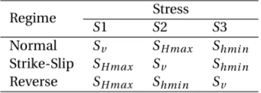
The relative magnitudes ofSv,SH max,Shmi n, determine the faulting regime in a stress system.
Anderson(1905) proposed a method to linkS1,S2,S3toSv,SH max,Shmi nand determine the local faulting regime, which is given in Table1.1.
1
2 1.INTRODUCTION Table 1.1: Anderson’s faulting theory linking magnitudes of in situ stress to principal stresses and faulting regimes.
Regime Stress
S1 S2 S3
Normal Sv SH max Shmi n Strike-Slip SH max Sv Shmi n Reverse SH max Shmi n Sv
1.2. I
N SITU STRESS IN BOREHOLESDrilling a borehole in the subsurface forces the stress trajectories to bend in such a way as to be parallel and perpendicular to the borehole wall (Kirsch,1898). Part of the rock mass is re- moved when a borehole is drilled, which is causing stress to concentrate around the borehole wall (Zoback,2007). Due to both processes, the ’hoop stress’ (σθθ), the stress acting circumferentially around the borehole, therefore bunches up in the direction of minimum stress at the borehole wall (Smi n) and spreads out in the direction of maximum stress at borehole wall (Smax), as can be seen in Figure1.1a. The hoop stress has extreme values at the borehole wall and stabilises rapidly with distance. In vertical boreholes,Smi nequalsShmi nandSmaxequalsSH max, in devi- ated boreholes this direct relationship does not hold, butSmi nandSmax are rotated variants of Shmi n,ShmaxandSv.
(a) Schematic overview of borehole with orientation ofSmi nand Smax, and the hoop stress (σθθ) acting around the borehole (after Zoback et al.(2003)).
(b) Breakout formation around borehole with respect to the orientation ofSmi nandSmax.
Figure 1.1: The relation between stress around a borehole and breakout orientation.
1.3. B
OREHOLE BREAKOUTSCompressive failure of the rock mass occurs at locations where the hoop stress exceeds the rock strength (Zoback et al.,1985). This is most likely to happen in the direction of minimum stress and therefore the regions where compressive failure occurs can be used as indicators for the di- rection ofSmi n andSmax. The regions where compressive failure occurs are called ’breakouts’
and are defined as cross-sectional elongations in the minimum stress direction, which are caused by localised failure around a borehole due to stress concentrations (Zoback et al.,1985). The re- lation between breakout location and stress direction is visualised in Figure1.1b. Breakouts are expected to extend along the borehole axis over depth and to form on opposite sides of the bore- hole, lining up withSmi n. Their width is related to the magnitude of the in situ stress (Zoback et al.,2003). For both vertical and deviated boreholes breakouts are used as indicators of the in
1.4.BOREHOLE BREAKOUT HETEROGENEITY 3
situ stress (Zoback,2007).
1.4. B
OREHOLE BREAKOUT HETEROGENEITYData from many wells shows that the presence, orientation, and shape of breakouts vary per loca- tion and over depth. Several mechanisms that cause breakout heterogeneity have been identified.
Shamir and Zoback(1992) found that the variations in breakout orientation can reflect stress fluc- tuations associated with active faults penetrated by the borehole. Breakout shape and orientation are systematically affected by the presence of natural fractures and fracture zones because the mechanical properties of the rock mass change in the surrounding rock (Sahara et al.,2014). The presence of natural fractures also suppresses or initiates breakouts to form, and influences the orientation of the breakouts (Lin et al.,2010). Mastin(1988) found that breakout orientation is influenced by the deviation of the drilled borehole from the vertical.
1.5. O
BJECTIVE OF STUDYThe objective of this study is to investigate the in situ stress and its variations around two deviated boreholes at BULG using the properties of breakouts present. By analysing breakout heterogene- ity we want to get a better idea about the causes of in situ stress variation. Knowledge gained on the section of the boreholes where breakouts are present will be used to extend our idea of the in situ stress and its variations in the vicinity of the boreholes and over their complete length. Since more boreholes will be drilled at BULG in the near future, the workflow used is designed to be applicable to data from other boreholes with varying properties.
Chapter2provides more information on the regional geology and the in situ stress in the prox- imity of BULG. Next to this we will introduce the geometry of BULG and the design of the bore- holes and measurement campaign. In Chapter3the presence of breakouts in the boreholes is analysed. This knowledge is used to identify patterns in breakout presence and breakout shape heterogeneity. Afterwards breakout presence will be related with the presence of natural fractures and fracture zones and borehole trajectories. Rock strength over depth is inverted based on ob- served breakout width. In Chapter4the theory behind breakout formation is extended over the whole length of the boreholes and the elliptical shape of the boreholes is used to gain knowledge on stress variations along the boreholes in zones that lack breakout presence.
2
S ITE DESCRIPTION AND TEST BOREHOLES
2.1. B
EDRETTOU
NDERGROUNDL
ABORATORY FORG
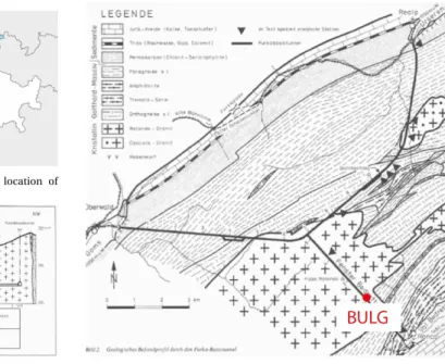
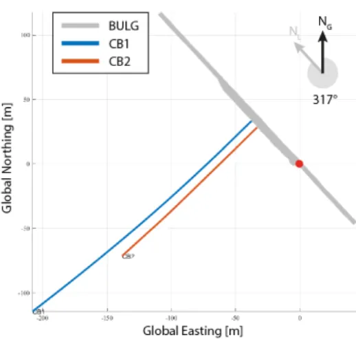
EOSCIENCES All data used for this thesis is obtained at the Bedretto Underground Laboratory for Geosciences (BULG). Figure2.1displays the location and geological setting of BULG. The laboratory is located in the Bedretto valley in the Swiss Central Alpine region, 10 km South-East of the town of Airolo, Ticino, Switzerland. It is located in an abandoned side access tunnel (the Bedretto Tunnel) to the Furka Base Railway Tunnel. The Bedretto tunnel has a total length of 5.2km, and has its own local distance ’tunnel meter’ (T M), which is set to zero at the South entrance of the tunnel. The BULG can be found in an enlarged cavern in betweenT M2000 andT M2100. The tunnel’s axis roughly follows the orientation of the mountain ridge above, trending in a NW-SE direction (317◦). A local coordinate system with origin at the southern start of the BULG (T M2000) is used next to the global coordinate system, and the local North (NL) is oriented parallel to the tunnel’s axis.The origin of the local coordinate system and the orientation ofNLare indicated in Figure2.3b.
The South entrance of the Bedretto tunnel has an altitude of 1480.5mabove sea level, and the overburden reaches a maximum of 1650munderneath the top of the Pizzo Rotondo (TM3100), the highest mountain of the Gotthard Massif. Above BULG the overburden has a thickness of 1000−1030m.
2.2. R
EGIONAL GEOLOGY AND IN SITU STATE OF STRESSThe stress regime in the larger Central Alpine region has been the subject of several studies, of which the results are displayed in Figure2.2. Figures2.2aand2.2bshow that bothHeidbach et al.
(2016) andKastrup et al.(2004) indicate a constrained, but non-uniform stress regime in the Cen- tral Alpine region. SH maxhas a general SE azimuth, but follows a progressive counterclockwise rotation from NE (Zürich) to SW (Geneva).Kastrup et al.(2004) show that the stress regime under- goes a transformation from a slight predominance of a strike-slip faulting regime in the foreland to a strong predominance of a normal faulting regime in the high parts of the Alps; the area where BULG is located.
5
6 2.SITE DESCRIPTION AND TEST BOREHOLES
BULG is located in the Gotthard Massif, and the local geology is dominated by Rotondo Granite.
Rotondo Granite is a relatively homogeneous massive light gray intrusion dating from the late phase of the Variscan Orogeny (Lützenkirchen and Loew,2011). During the Variscan methamor- phosis, the Rotondo Granite received its sub-vertical foliation, which has a NE azimuth (Lützenkirchen and Loew,2011). The orientation and dipping angle of the foliation match with fault zones in- tersecting the Bedretto tunnel perpendicularly. Research done at the nearby Gotthard pass area shows that the orientation of the fault zones is consistent over the larger area (Zangerl et al.,2006).
(a) Map of Switzerland with indicated location of BULG.
(b) Cross section of the Bedretto tunnel with indicated location of BULG.
(c) Geological map of Bedretto tunnel with indicated location of BULG.
Figure 2.1: The location and geological setting of BULG. Modified fromKeller and Schneider(1982).
(a) World Stress Map (WSM) data available of the Central Alps (Heidbach et al.,2016).
(b) Compiled stress data inverted from earthquake focal mechanisms (Kastrup et al.,2004).
Figure 2.2: Available stress data for the larger Central Alpine region.
To obtain an estimation of the magnitude of the in situ stresses at BULG, three vertical bore- holes of 30mlength have been drilled and were logged and analysed by Ma et al.(2019) and Broeker(2019). After running mini-frac tests in the boreholes, induced hydraulic fractures dip- ping approximately 80◦were visible on image logs, suggesting that the assumption of overbur- den stress being vertical is practically sufficient (Ma et al.,2019). Using the density of Rotondo
2.3.BOREHOLES AND DATA ACQUISITION 7
Granite and the average overburden thickness at BULG,Sv is estimated at 26.5M P a, and using tensile fractures the orientation ofSH maxis estimated at 100◦. Based on mini-frac experiments, Broeker(2019) estimated rangesShmi n=12.6−15.2M P a,SH max=17.8−23.8M P aand addition- allyPp=2.4−5.3M P a.
2.3. B
OREHOLES AND DATA ACQUISITIONIn September 2019 three 97mm diameter boreholes were completed at BULG;C B1,C B2, and C B3. This study focuses on boreholeC B1 andC B2 only, since both have been logged using an Acoustic Televiewer (ATV) tool. Properties of both boreholes are given in Table2.1and the trajec- tory of both boreholes is displayed in Figure2.3. The ATV probe emits an acoustic signal towards the borehole wall and provides a detailed image of the borehole wall based on the amplitude and travel time of the reflected signal. The data sets gathered contain amplitude and travel time data in the angular resolution for each depth in vertical resolution. Two ATV logs were obtained for C B1 and one ATV log was obtained forC B2. Information on all ATV logs can be found in Ta- ble2.2. During the acquisition of each ATV log an azimuth log, tilt log, and caliper log were also obtained. The azimuth log measures the exact orientation of the borehole over depth, the tilt log measures the deviation of the borehole from the vertical axis over depth, and the caliper log records the maximum and minimum diameter of the borehole over depth.
(a) Side view of CB boreholes and BULG plotted in local coordinate system.
(b) Top view of CB boreholes and BULG plotted in global coor- dinate system. The magnetic North is indicated as NGand the local North is indicated as NL. The origin of the local coordi- nate system is indicated by the red dot.
Figure 2.3: Location and trajectory of the CB boreholes and BULG.
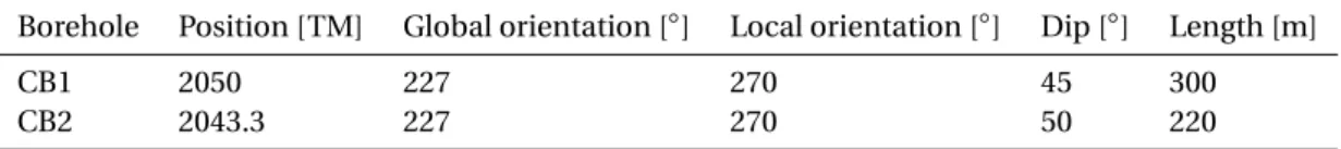
8 2.SITE DESCRIPTION AND TEST BOREHOLES Table 2.1: Properties of used boreholes.
Borehole Position [TM] Global orientation [◦] Local orientation [◦] Dip [◦] Length [m]
CB1 2050 227 270 45 300
CB2 2043.3 227 270 50 220
Table 2.2: Properties for used ATV logs.
Name Borehole Logging date Vertical resolution [m] Angular resolution [◦]
ATVCB1.1 CB1 2019.12.11 0.01 2.5
ATVCB1.2 CB1 2020.05.13 0.01 1
ATVCB2.1 CB2 2019.12.11 0.01 2.5
3
B REAKOUT ANALYSIS
In this Chapter we discuss variations in breakout presence, orientation and shape, and the un- derlying processes that cause these variations. Because breakouts are indicators of the in situ stress, we can infer from them what variations of the in situ stress are present in the subsurface.
Breakout and fracture interpretation was done in borehole logging software WellCAD, statistical analysis and modeling was performed in MATLAB. Several plots in this Chapter display results based on orientation. One should note that in this Chapter 0◦, or North, refers to the top of the borehole when looking downhole. The abbreviation used to indicate this coordinate system is
’HS’. In AppendixAthe same plots are displayed but with 0◦, or North, referring to the magnetic North, for which the abbreviation ’NM’ is used. The depth indicated in all plots is borehole depth (BHD). Several plots show ’average’ data. This means that the data visualised is treated with an average filter with a moving window of 2m, which was done to smooth profiles.
3.1. B
REAKOUT OBSERVATIONSAs discussed in Section1.3, breakout orientation corresponds to the direction ofSmi n, and break- out width corresponds to the magnitude of the in situ stresses. By analysing trends in breakout orientation and width over depth we get an image of variations of the in situ stress over depth.
3.1.1. M
ETHODSBreakouts are identified based on Acoustic Televiewer (ATV) logs ran over the whole length of the boreholes. The ATV logs were acquired several months after the drilling had finished, therefore the effect of time-dependent breakout widening is no longer significant, but an increase in depth is possible (Schoenball et al.,2014). The breakouts are picked manually based on the amplitude response of the ATV log, where breakouts show up as zones of low amplitude, as can be seen in Figure3.1. The azimuth of the breakout’s centre and breakout widths were picked every 20cm over the borehole length. This approach enables us to examine different breakout properties sta- tistically and correlate the breakout presence with the presence of fractures and faults later on. A comparison of the 20cmdata with data picked over varying intervals is shown in AppendixB.1.
9
10 3.BREAKOUT ANALYSIS
Breakouts can be confused with washouts, keyseating, or drilling-induced tensile failure when picked manually from ATV data and therefore the breakouts picked need to satisfy certain con- straints. The data is only used for further analysis if the breakout width exceeds 5◦.
To separate the breakouts from keyseating and washout phenom- ena the maximum caliper should increase more than 1% of the bore- hole diameter and the minimum caliper should indicate the bore- hole diameter (Plumb and Hick- man,1985).
A separation is made between breakouts that form breakout pairs and single breakouts. To form a ’breakout pair’ two breakouts must be located at the same depth and the difference of their azimuth should be larger than 130◦. If this is not the case, the breakout is treated as a ’single breakout’. An example of breakouts treated as a single breakout or as a breakout pair is shown in Figure3.1.
Figure 3.1: Breakout presence on ATV amplitude log and caliper log.
Breakouts are visible as zones with low amplitude, where the maxi- mum caliper increases but the minimum caliper matches the borehole diameter. Examples of a single breakout and a breakout pair are indi- cated.
3.1.2. R
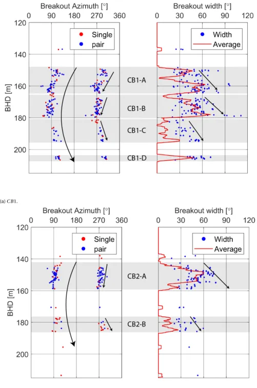
ESULTSIn boreholeC B1, 262 breakouts are identified, concentrated in a zone between 120−220mBHD.
The mean orientation ofSmi nindicated by the breakout azimuths is N95◦±16◦E and the break- outs have a mean width of 50◦±17◦. 101 breakout pairs are counted, together with 60 single breakouts. As can be seen in Figure3.2a, both single breakouts and breakout pairs follow the same azimuth trend. The single breakouts are divided evenly over both sides of the borehole (48%−52%) and have a mean width of 40◦±17◦, significantly lower than the overall mean width.
On the scale of the interval between 120−220mBHD the breakout azimuth rotates counterclock- wise from 110◦(150mBHD) to 70◦(180mBHD) and clockwise back to 110◦(205mBHD), as indi- cated in Figure3.2a. On a smaller scale, the breakouts can be divided into four groups (C B1A−D) based on trends in azimuth and width. All four groups including their trends are visualised in Figure3.2a.C B1−AandC B1−Bshow a counterclockwise rotation in the azimuth over depth, whereC B1−C shows a clockwise rotation.C B1A−C all show an increase in width over depth.
C B1−Ddoes not show trends in azimuth and width, but constant and stable values for both.
InC B2 136 breakouts were identified in the lower part of the borehole (120−220mBHD), indi- cating an orientation of N95◦±13◦E forShmi n. The mean breakout width is 48◦±15◦, 47 breakout pairs and 40 single breakouts are counted. Single breakouts dominate the deeper part of the in- terval with the majority (60%) located on the Eastern half of the borehole (N0◦−180◦E). The single breakouts are characterised by a smaller mean width of 38◦±15◦.
Figure3.2bshows us that a rotating trend is present in azimuth over the interval, rotating coun- terclockwise from 105◦(145mBHD) to 80◦(170mBHD) and clockwise back to 105◦(180mBHD),
3.1.BREAKOUT OBSERVATIONS 11
although breakouts are not present at the center of this rotation. Smaller trends are identified for two groups of breakouts,C B2A−B.C B2−Ais characterised by a counterclockwise rotation of the azimuth, andC B2−Bby a clockwise rotation. In both intervals the breakout width increases over depth.
(a)C B1.
(b)C B2.
Figure 3.2: Breakout azimuth and width forC B1 andC B2, zoomed into interval between 120−220mBHD. Single breakouts and breakout pairs are indicated. Azimuth trend over the complete borehole is indicated, as well as trends in azimuth and width for groups of breakouts identified,C B1A−DandC B2A−BforC B1 andC B2 respectively. Breakout azimuth is given with respect to top of borehole (HS), orientation with respect to magnetic North (NM) is displayed in AppendixA.1.
12 3.BREAKOUT ANALYSIS
3.2. B
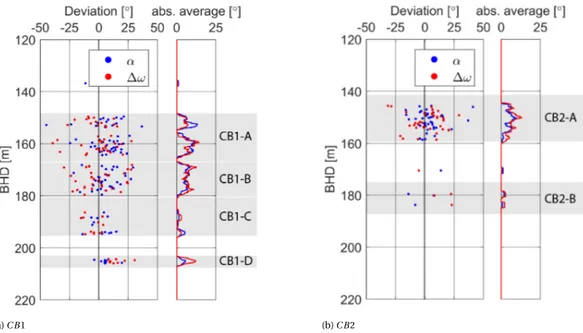
REAKOUT SHAPE ANALYSISBreakout pairs are expected to develop symmetrically on opposite sides of the borehole, match- ing with the azimuth ofSmi n as illustrated in Figure1.1b. In boreholesC B1 andC B2 however, breakout pairs were observed to be asymmetrically formed.
Breakout pair asymmetry is an indicator of the presence of local weak zones, caused by fractures or drilling process, around the borehole of which the geo-mechanical properties are modified (Sahara et al.,2014).
3.2.1. M
ETHODSTo investigate variations in breakout shape all breakout pairs were analysed. For each breakout pair the orientation devia- tion given by angle α was calculated to- gether with the width deviation∆ω=ω1− ω2. A1andω1correspond to the azimuth and width of the breakout located on the N0◦−180◦Ehalf-circle. A positive value of αindicates clockwise rotation ofA2with re- spect to A1. The absolute values ofαand
∆ωare stored to be used later on.
Figure 3.3: Schematic overview of borehole with het- erogeneous breakouts. Indicated are breakout az- imuthsA1andA2, the orientation deviation given by angleαand breakout widthsω1andω2.
3.2.2. R
ESULTS(a)C B1 (b)C B2
Figure 3.4: Orientation deviation (α) and width deviation (∆ω) for breakout pairs inC B1 andC B2, zoomed into interval between 120−220mBHD.αand∆ωare displayed for each breakout pair, as well as the average of the absolute values for bothαand∆ω, indicating the relative amount of deviation over depth. Breakout groups as discussed in Section3.1, are displayed for both boreholes.
3.3.BREAKOUT CORRELATION WITH PRESENCE OF NATURAL FRACTURES AND FRACTURE ZONES 13
Figure3.4shows us that breakout pairs in both boreholes with low orientation deviationαcome with low width deviation∆ω. InC B1 75% of the breakout pairs giveα>0, showing a preference forA2to rotate clockwise with respect toA1, although breakout groupC B1−Cis an exception on this trend, showing no preference. 50% of∆ω>0, indicating that the widest breakouts of pairs are divided evenly over both sides of the borehole. The breakout pairs in groupC B1−D form an exemption on this trend because for all pairsω1>ω2. When interpreting the breakout shape analysis forC B2, one should note that the results do not contain much information on breakout groupC B2−B, since this group is dominated by single breakouts. 50% of the breakout pairs give α>0, indicating no preferred rotation direction ofA2with respect toA1. 60% of∆ω>0, indicating a slight preference forω1to be bigger thanω2.
3.3. B
REAKOUT CORRELATION WITH PRESENCE OF NATURAL FRAC-
TURES AND FRACTURE ZONES
The presence of fractures can influence the azimuth of breakouts. Shamir and Zoback(1992) showed that active faults cause stress perturbations, and calculated that breakout orientation variations need an extreme local stress drop.Sahara et al.(2014) conclude that breakout orienta- tion variation in the vicinity of fracture zones reflects the large scale stress heterogeneity due to geo-mechanical changes caused by the fracture zones. The presence of single fractures is able to cause heterogeneity for both stress orientation and magnitude as well (Lin et al.,2010).
3.3.1. M
ETHODSFractures intersecting the boreholes were identified using ATV logs and optical televiewer (OTV) logs. The OTV probe emits light on the borehole wall and produces 360◦photo images of the borehole wall which are continuous over depth. Fractures show up as sinusoidal curves in both ATV and OTV logs that can be picked, after which the depth, apparent dip direction, and apparent dipping angle are stored. The presence of fractures on ATV and OTV logs, together with the picking process, is shown in Figure3.5.
Table 3.1: In situ stress regime and ad- ditional parameters used to calculate slip tendency on fractures in boreholesC B1 andC B2.SvandPpincrease with increas- ing depth.
Parameter Value
S1/Sv(0mBHD) 26.5 MPa S2/SH max 0.95∗S1 S3/Shmi n 15.2 MPa Pp(0mBHD) 3 MPa S1azimuth N100◦E
µ 0.68
Figure 3.5: Fracture presence on ATV log and OTV log. Both logs show an example of a fracture intersecting the borehole and a picked fracture. In 3D a fracture is a plane intersecting the borehole, which is described by the strike and the dipping angle (φ).
14 3.BREAKOUT ANALYSIS
Knowledge of the orientation and tilt of the borehole enables us to transform the apparent dip di- rection and apparent dipping angle to the true dip direction and true dipping angle; true meaning with respect to the magnetic North and the horizontal. As illustrated in Figure3.5, the strike can be derived by deducting 90◦from the dip direction. Strike and dipping angle combined give us the fracture plane, of which we can calculate the slip tendency using the following formula:
Ts= τ σn
. (3.1)
In equation3.1,Tsrefers to the slip tendency, and sliding occurs ifTs≥µ, the coefficient of fric- tion. With knowledge of the in situ stress regime the magnitudes ofτ, the shear stress, andσn, the effective normal stress acting on the fracture plane, can be calculated using tensor transforma- tion (Zoback,2007). The in situ stress regime used is based on estimations fromBroeker(2019) andMa et al.(2019), and is given in Table3.1. The pore pressure,Pp, and the magnitude ofSvare recalculated for each fracture since they increase over depth. The values given in Table3.1are the starting values used at BHD=0m.
The influence of fractures on breakout presence, orientation, and shape was investigated on two scales. On a large scale (>20m), zones with a high fracture density are treated as fracture zones, of which the influence is investigated. On a small scale (10m) we looked at the influence of fracture presence on different breakout groups present in the boreholes.
3.3.2. R
ESULTSOver the whole length ofC B1 240 fractures have been identified which are displayed together with their properties in Figure3.6a. 75% of the fractures has an apparent dip direction towards North (N315◦−20◦E HS) and 25% towards Southeast (N90◦−180◦E HS). The mean apparent dip- ping angle is 60◦±15◦.The fracture density is higher in the zone where breakouts are present and reaches a maximum of 7 fractures/meter (195mBHD) close the bottom of the breakout zone (205mBHD). The slip tendency, calculated based on the true dip direction and true dipping angle, reaches maximum values atTs=0.35, and therefore no active faults are present inC B1 (Ts(max.
0.35))<µ(0.68)).
Figure3.6shows that breakout presence comes with high fracture density. Figure3.7displays fracture density over the interval between 120−220mBHD, together with several breakout prop- erties. In Figure3.7awe seeC B1−Ais characterised by decreasing fracture density and increasing breakout density,C B1B−Cby increasing fracture density and breakout density, andC B1−Dby the lack of fractures but high breakout density.
InC B2 123 fractures have been identified, which are displayed together with their properties in Figure3.6b. The majority (65%) of the fractures show an apparent dip direction towards North (HS), and a secondary group of fractures (35%) is visible with an apparent dip direction towards the Northeast (HS), with a mean apparent dipping angle 60◦±10◦. The fracture density reaches a maximum of 7 fractures per meter in the zone where breakouts are present, at the bottom of each breakout interval. The maximum slip tendency calculated isTs=0.35, and therefore no active faults are present inC B2 either.
Figure3.7bshows that both breakout groups,C B2−AandC B2−B, are characterised by increasing fracture density and constant breakout density, although the breakout density inC B2−Bis much lower than inC B2−A. Figure3.7aand3.7btogether show that each breakout group in bothC B1 andC B2 is bounded by a (local) minimum in fracture density on top and a (local) maximum
3.3.BREAKOUT CORRELATION WITH PRESENCE OF NATURAL FRACTURES AND FRACTURE ZONES 15
in fracture density at the bottom, with two exemptions;C B1−Awhere the fracture density gets smaller over depth, andC B1−D where no fractures are present. C B1−C andC B2−B show that orientation deviation and width deviation are more influenced by breakout density than by fracture density.
(a)C B1 (b)C B2
Figure 3.6: Fracture presence, properties and statistics inC B1 andC B2. Apparent dip directions are indicated for each fracture where the colour indicates the apparent dipping angle, as indicated in the colour bar. The fracture density over depth is indicated as well as the slip tendency calculated for each fracture, corresponding to the two additional x-axes on the bottom of the plot. Indications are given for the location of the zone with breakout presence and the zone used in zoom-in plots in blue and red respectively. The same plots but containing true dip direction and true dipping angle can be found in AppendixA.2.
(a)C B1 (b)C B2
Figure 3.7: Fracture density compared with breakout properties inC B1 andC B2, zoomed into interval between 120−220m BHD. All plots display averaged values and trends are indicated for each breakout group.
16 3.BREAKOUT ANALYSIS
3.4. B
REAKOUT CORRELATION WITH BOREHOLE TRAJECTORYAs can be seen in Figure2.3a, the deviation from the vertical (the tilt) increases around 10◦over depth for both boreholes. This means that the orientation of the borehole wall with respect to the in situ stress changes over depth. This orientation is of influence on the presence, azimuth, and shape, of breakouts, since the magnitude and orientation of the stresses acting at the borehole wall change.
3.4.1. M
ETHODSFollowingBroeker(2019) andMa et al.(2019) we assume that the faulting regime around BULG is Normal Faulting/Strike-Slip. Using the stress ratio around BULG, given by (S2−S3)/(S1−S3)= 0.95, and the deviation of the borehole orientation with respect to the orientation ofSH max, the relation described byMastin(1988) predicts considerable change in breakout azimuth.
The direct link between borehole orientation, borehole tilt, and breakout presence is investigated, as well as the influence of the rate of change of the orientation and tilt. The rate of change is expressed as
Rz= xz
xz−∆z, (3.2)
where each value of current interestxz is compared to a value at a certain depth interval (∆z) abovexz−∆z. IfRz>1, this means the tilt or orientation has increased over∆z.
3.4.2. R
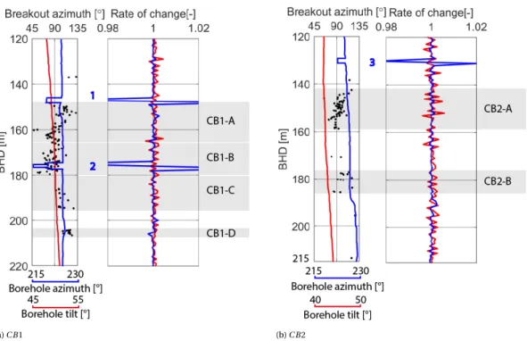
ESULTS(a)C B1 (b)C B2
Figure 3.8: Average borehole azimuth and average borehole tilt over the intervals 120−220mBHD and 120−215mBHD for boreholesC B1 andC B2 respectively. Rate of change for azimuth and tilt are also displayed (based on∆z=1m). Breakout azimuths are plotted (HS) and breakout groups are indicated. Anomalies in borehole azimuth are highlighted by 1, 2 for C B1 and by 3 forC B2.
Breakout azimuth, borehole azimuth and borehole tilt are displayed together with their rate of change (calculated for∆z=1m) and the breakout groups in Figure3.8for bothC B1 andC B2, over the interval between 120−220mBHD. In Figure3.8awe see that the tilt ofC B1 is gradually
3.5.ROCK STRENGTH INVERSION FROM BREAKOUT PRESENCE 17
increasing over depth, from 48◦to 51◦. This could cause a rotation of the breakout azimuth to- wards the horizontal of several degrees (<5◦). The borehole azimuth stays constant over depth at 227◦(NM), but shows two anomalies where the azimuth decreases heavily for a short interval, indicated by 1 and 2.C B1−Ainitiates after anomaly 1, andC B1−Bterminates after anomaly 2.
InC B1−Cthe azimuth is constant, where inC B1−Dit shows a very light variation.
InC B2, the tilt increases from 47◦to 49◦over the interval 120−215mBHD, as can be seen in Figure 3.8b. This increase can result in a small rotation of the breakout azimuth towards the horizontal, as discussed above. The borehole azimuth increases gradually over depth, showing an anomaly at 130mBHD, indicated by 3 in Figure3.8b. In both breakout groupsC B2−AandC B2−Bborehole tilt and borehole azimuth increase at a constant rate.
3.5. R
OCK STRENGTH INVERSION FROM BREAKOUT PRESENCEBreakout width is related to rock strength, the orientation of the borehole, and in situ stress (Zoback et al.,2003). Using estimations of the in situ stress together with breakout observations, estimations can be made on the rock strength in areas with breakout presence.
3.5.1. M
ETHODSFor a normal faulting regime, the in situ stress can be described by the orientation of SH maxand the stress tensor
Ss=
Sv 0 0
0 SH max 0
0 0 Shmi n
, (3.3)
containing the magnitudes of the three principal stresses. Using tensor transfor- mations (Jin,2018), knowledge of the pore pressure and the orientation and dipping angle of the borehole, tensorSs can be ro- tated into tensor
Sb=
σ11 τ12 τ13
τ12 σ22 τ23
τ13 τ23 σ33
. (3.4)
Figure 3.9: Orientation of effective normal stresses with respect to borehole.σ11is aligned with the bore- hole axis,σ22points to the bottom of the cross section, σ33is aligned with the horizontal crossing the cross section.θ, rotating counterclockwise around the bore- hole is also indicated.
In tensorSb,σ11,σ22,σ33are the effective normal stresses, and line up with the borehole axis, with the radial pointing to the bottom of the cross section, and along the horizontal intersecting the borehole cross section (Zoback et al.,2003). The orientation ofσ11,σ22,σ33with respect to the borehole is visualised in Figure3.9.τ12,τ13,τ23are the shear stresses acting orthogonally to directions of the normal stresses. Assuming linear elastic behaviour up to the point of failure of an homogeneous isotropic rock (Peška and Zoback,1995), the Kirsch equations (Kirsch,1898) can be used to calculate the magnitude of the hoop stress (σθθ) at the borehole wall for an arbitrary angleθusing the following equation:
σθθ=σ11+σ22−2(σ11−σ22)cos2θ+4τ12si n2θ−∆P. (3.5)
18 3.BREAKOUT ANALYSIS
In Equation3.5θis an arbitrary angle at the borehole wall, equal to 0◦at the bottom of the bore- hole, increasing counterclockwise (down hole) to 360◦as illustrated in Figure3.9.∆Pis the differ- ence between the pore pressure and the drilling fluid pressure, which was zero in this project.
As mentioned in Section1.3, breakouts appear at locations around the borehole whereσθθex- ceeds rock strengthC0. Using the stress regime given in Table3.1and Equation3.5the magnitude ofσθθcan be calculated for each location (0◦≤θ≤360◦) around the borehole. Breakout width can be calculated now as the sum of all values ofθfor whichσθθ>C0, divided by 2, since break- outs are expected to appear in pairs. This direct link was used to estimate the magnitude ofC0 of the rock mass surrounding both boreholes based on observed breakout widths.
3.5.2. R
ESULTSThe simulations in this Section are based on the in situ stress as described in Table3.1, whereSv andPp are adjusted to the depths showing maximum breakout frequency; 180mBHD forC B1 and 150mBHD forC B2. Using Equation3.5the breakout widths (WBO) for different values ofC0 were calculated, which are displayed in Figure3.10, where they are compared with the observed maximum, minimum and mean breakout width. The difference betweenC B1 andC B2 is their dipping angle, which is 45◦forC B1 and 50◦forC B2.
As discussed in Section3.1, the mean breakout width inC B1 is 50◦±17◦, which corresponds to C0=50.3M P a, indicated in Figure3.10atogether with the standard deviation highlighted in grey.
The maximum breakout width observed is 111◦at 179MBHD and corresponds toC0=37.1M P a, the minimum breakout width of 16◦is observed very close to the maximum value, at 183mBHD, and corresponds toC0=54.4M P a. The mean breakout width inC B2 is 48◦±15◦, corresponding toC0=50.0M P a, as indicated in Figure3.10b. InC B2, the maximum breakout width of 76◦is reached at 155mBHD, indicatingC0=45.4M P a. The minimum breakout width is 17◦at 144m BHD, indicatingC0=53.1M P a.
(a)C B1 (b)C B2
Figure 3.10: Estimated breakout width (WBO) calculated for different magnitudes ofC0 forC B1 andC B2. The estimated breakout width values are displayed and compared with the observed meanWBO, the standard deviation, the maximum WBOand the minimumWBO, for which the corresponding values ofC0 are indicated. Simulation is based on in situ stress given in Table3.1, and adjusted for 180mBHD inC B1 and for 150mBHD inC B2.
Using the method described above, we can use the average breakout width inC B1 andC B2 to investigate trends inC0 over depth. Because this method is based on breakout presence, the results focus solely on zones where breakouts occur. Therefore the results shown are displayed for the interval 120−220mBHD. The results of this simulation are visualised in Figure3.11, where
3.6.DISCUSSION 19
the calculated magnitude ofC0 over depth is displayed together with the average breakout width.
For bothC B1 andC B2 the calculated magnitudes ofC0 vary between 48−55M P a, and zones with lowC0 are related to zones with high breakout width. C0 varies more heavily in borehole C B1, and the magnitude ofC0 is lower in general inC B2, when compared toC B1.
In Figure3.11awe see that in the zones around breakout groupC B1A−Cthe magnitude ofC0 decreases over the interval, with maximum values located at the top of each interval and min- imum values located at the bottom of each interval. C B1A−Bindicate lower magnitues ofC0 thanC B1−C. No clear trend is visible in breakout groupC B1−D. Figure3.11bshows that in the zone around breakout groupC B2−Athe lowest values ofC0 are present in the middle of the interval. We see that the magnitude ofC0 is relatively high around breakout groupC B2−B, but decreases over depth, reaching a minimum value at the bottom of the interval.
(a)C B1 (b)C B2
Figure 3.11: Magnitude ofC0 over the interval between 120−220mBHD forC B1 andC B2, based on breakout width. This method is based on breakout width and therefore only values forC0 are shown in zones where breakouts are present. The average breakout width over depth is displayed together with calculated magnitudes ofC0, which are indicated by the shaded zones of which the colors relate to the magnitude. For both boreholes the breakout groups are indicated.
3.6. D
ISCUSSIONIn a homogeneous in situ stress field, no variation in breakout appearance is expected (Zoback et al.,1985). The breakouts occurring in boreholesC B1 andC B2 show variation in presence, azimuth and shape over depth, indicating the in situ stress field around the boreholes is hetero- geneous on several different scales (Schmitt et al.,2012).
Both boreholes show a zone with a relatively high fracture density. This zone is located over the intervals 140−190mBHD inC B1 and 135−180mBHD inC B2. Zones with high fracture density can either be fracture zones or fault zones, based on their slip tendency. If the slip tendency (Ts) exceeds the coefficient of friction (µ) for fractures present the zone is treated as a fault zone, and slip on the fractures results in rotations of the breakout azimuths (Paillet and Kim,1987;Shamir and Zoback,1992). Based on calculations made this is not the case for the fractures present and therefore we will treat the zone with high fracture density as a fracture zone.
Fracture zones are expected to come with perturbed and rotated stresses depending on the change in elastic properties of the damaged rock (Sahara et al.,2014). The maximum stress per-
20 3.BREAKOUT ANALYSIS
turbation will be reached in the core of the fractured zone, since this is where most damage is done. Breakouts are stress indicators and therefore we can use their presence to locate the core of the fracture zone. The rotation in breakout azimuth inC B1 reaches its maximum of 40◦at 180mBHD, this is where the core of the fracture zone is located. InC B2 the maximum rotation in breakout azimuth of>25◦is reached at 170mBHD, although very few breakouts are present at this depth, which can be caused by the suppression of breakouts by fractures (Lin et al.,2010).
The fact that a fracture zone causes rotation of breakout presence also means that breakouts present above/below the fracture zone are a trustworthy indicator for the orientation ofSmi n, which we can use to determine the orientation ofShmi n. An orientation of N105◦E (HS) ofSmi n corresponds to an orientation ofShmi n equal to N190−195◦E (NM) for a borehole deviated 45◦ (Mastin,1988). This orientation agrees with earlier findings ofMa et al.(2019);Broeker(2019).
FromMastin(1988) we can derive that the increasing tilt of bothC B1 andC B2 will result in a counterclockwise rotation of the breakout azimuth. In both boreholes however we also witness clockwise rotation trends, indicating that the main drive behind the rotation in breakout azimuth is the fracture zone and not borehole trajectory. The anomalies present in the borehole trajectory data have not been of influence on breakout presence, but can be used as indicators for geo- mechanical boundaries (Morton-Thompson and Woods,1993).
Breakouts are present in 6 groups over both boreholes, characterized by an increase in breakout width followed by a steep decline in width. In 4 groups identified, fracture density and breakout density increase with increasing breakout width. The presence of zones with varying fracture densities can be explained by the presence of mechanical layering around fracture zone cores (Bauer et al.,2015). The fracture density influences the mechanical properties of the rock mass (Faulkner et al.,2007) and therefore influences breakout width. Contrary to the findings ofSahara et al.(2014), breakout shape heterogeneity is not following the same trend as fracture density in boreholesC B1 andC B2. Breakout groups located above the core of the fracture zone show larger breakout widths than the breakout groups located under the core suggesting the rock mass is more influenced by the fracture zone above its core than under its core.
Based on breakout width, the estimated in situ stress and borehole trajectory, the calculated mag- nitude of C0 varies over depth, approaching local minima at the bottom of each breakout group.
This suggests that a higher fracture density is related to a lower rock strength. The mean C0 is estimated at 50M P a, which is considerably lower than the rock strength of intact granite, esti- mated at 170M P a. Decreases in rock strength of this magnitude are not uncommon for densely fractured rock mass (Villeneuve et al.,2018;Shamir and Zoback,1992). Although this method can be used to get an estimation on the magnitude ofC0 it is important to note that the mechanisms that control the failure evolution of the borehole wall are not well understood and based on as- sumptions for homogeneous rock. The relation used is based on the common assumption that breakouts do not widen but only deepen until the borehole reaches a new stable state (Zoback et al.,2003), but (Azzola et al.,2019) shows that the width does increase over time. Since the data sets used for this research were obtained several months after drilling, the breakout width might not reflect the in situ stress.
Based on all properties inspected, and especially on the comparability of breakout groupsC B1− A,C B1−BandC B2−A, it is likely that the fracture zone intersectingC B1 and the fracture zone C B2 are in fact the same fracture zone. From this follows a limitation on this study; because just one fracture zone is investigated, the conclusions drawn cannot be generalised to fracture zones in general.
4
B OREHOLE ELLIPTICITY ANALYSIS
Breakouts provide very useful insight in in situ stress heterogeneity and its causes, but are only present at 25% of the borehole lengths ofC B1 andC B2. It was supposed that the mechanism behind breakout formation is already acting before breakouts form and influences the borehole shape. It will cause the borehole to get an elliptical shape, and the long axis of the ellipse lines up with the orientation ofSmi n. Therefore a detailed analysis of the borehole shape of both bore- holes was conducted. Borehole ellipticity is used to automatically analyse breakout orientation (Valley and Evans,2009), but the interest of this study is the influence of the in situ stress on the borehole shape in borehole intervals that lack breakout presence. The analysis is based on ATV log travel time data which is imported using borehole logging software WellCAD, the data is after- wards analysed in MATLAB.
One should note that in this chapter 0◦, or North, refers to the top of the borehole when looking downhole. The abbreviation used to indicate this coordinate system is ’HS’. In AppendixAthe same plots are displayed but with 0◦, or North, referring to the magnetic North, for which the abbreviation ’NM’ is used. The depth indicated in all plots is borehole depth (BHD).
4.1. M
ETHODSThe ATV log travel time data contains transit time from the probe to the borehole wall and back in microseconds. The standard procedure is to centralize travel time data in WellCAD before analysing the data (ALT,2019), but it is essential for our analysis that this process is not applied to the travel time data. This is because the ’centralise process’ removes sinusoidal trends from the data, but these sinusoidal trends contain all information on borehole ellipticity. A comparison between results gained from centralised data and results gained from original data is displayed in AppendicesB.2andB.3.
To reduce noise present the data was treated with an average filter with a moving window of 0.2m.
Travel time data is saved each 20cmover the borehole length, matching the breakout data which is stored over the same interval (see Section3.1). The data is converted from travel time to borehole radius using
r(θ,z)=∆t(θ,z)∗vm(z)∗10−6
2 +rp, (4.1)
21
22 4.BOREHOLE ELLIPTICITY ANALYSIS
where radiusr is calculated at depthzand angleθ around the borehole, using travel time ∆t(θ,z), acoustic velocity through drilling fluidvm, and the radius of the ATV proberp. Using goniometry,r can be con- verted to the x-y coordinates of the respec- tive point at the borehole wall. Using least squares fitting (Halir and Flusser,1998) an ellipse is fitted to the set of x-y coordinates corresponding to the location of the bore- hole wall for all anglesθat a specific depth, representing the cross section of the bore- hole at that depth. The orientation of the ellipse long axis is determined, and the el- lipticity ratio is derived as
R=a0
b0, (4.2)
Figure 4.1: (Exaggerated) expected shape of borehole with respect to in situ stress. The fitted ellipse is dis- played as the dashed ellipse, witha0andb0its short axis and long axis respectively.
wherea0 andb0 correspond to the minor axis length and the major axis length respectively. A lower value ofRcorresponds to a more elliptical borehole shape. A schematic overview of the assumed shape of the borehole with respect to the in situ stress and the fitted ellipse together with its axesa0andb0is shown in Figure4.1.
4.2. R
ESULTSThe results shown in this Section are based on data setsAT V C B1.2 andAT V C B2.1, of which the properties are given in Table2.2.
For both logs,rp =0.95cmandvmwas set equal to 1450m/s, the acoustic velocity in water.
The developed method was first applied to a single depth interval of 20cm located in C B1 at 150.2mBHD. This interval was cho- sen because of the clear presence of break- outs, as can be seen in Figure4.2 , where the calculated cross section is displayed together with the determined azimuth of the major axisb0 and breakoutsBO1 and BO2. We see that the determined azimuth of 112.6◦lines up with the azimuth ofBO2, but is deviated from the azimuth ofBO1 by 5◦.
Figure 4.2: Calculated cross section ofC B1 together with the determined azimuth of the ellipse long axis b0. The cross section displayed is calculated based on ATV log travel time data over the 20cminterval around 150.2mBHD inC B1. The determined azimuth of the ellipse long axis (b0) is matches exactly with the az- imuth of breakoutBO2 and approaches the azimuth of breakoutBO1.
4.2.RESULTS 23
The fitting algorithm can thus be used to estimate the orientation ofSmi nover this depth interval, but is not able to detect small scale variations.
As discussed in Chapter1, breakouts are indicators of the orientation ofSmi n. The azimuth of the ellipse long axis was determined over the interval where breakouts occur, 120−220mBHD 120−215mBHD forC B1 andC B2 respectively, to see if the ellipse long axis follows the same trend over depth as the breakouts do. Figure4.3shows the one-sided breakout azimuth plot over the intervalsC B1 andC B2, together with the determined azimuths ofb0for each interval depth.
Both forC B1 andC B2 we see that the azimuth ofb0follows the trends present in the breakout azimuth over depth, as described in Section3.1. At interval depths where breakouts are present the difference in breakout azimuth and ellipse long axis azimuth was calculated, with a mean difference of 4◦forC B1 and a mean difference of 7◦forC B2. In Figure4.3awe see that the azimuth ofb0shows several outliers from the general breakout trend inC B1, which are spread randomly over depth. Figure4.3bshows that inC B2 there are two zones (Z1,Z2) where the azimuth ofb0 and the trend ofb0over depth differ structurally from the breakout azimuth and trend. InZ1 the breakout orientation rotates counterclockwise, but the azimuth ofb0rotates clockwise. InZ2 the breakouts are located around 100◦, where the azimuth ofb0is estimated at 80◦.
(a)C B1 (b)C B2
Figure 4.3: Breakout (BO) azimuth and ellipse long axis (b0) azimuth forC B1 andC B2 over the intervals 120−220mBHD 120−215mBHD respectively. Outliers ofb0azimuth with respect to the trend of the breakout azimuth are spread randomly over depth inC B1. InC B2 we see that two zones (Z1,Z2) are present where the azimuth ofb0and the trend of the azimuth ofb0structurally differs from the breakout azimuth and its trend. Breakout azimuth and ellipse long axis are given with respect to the borehole top (HS), azimuth with respect to magnetic North (NM) is displayed in AppendixA.3.
Figures4.4and4.5display the azimuth ofb0and the ellipticity ratioRover the complete length of the boreholes for boreholeC B1 andC B2 respectively. Note that the scale given forRinC B1 ranges 0.98−1, and the scale forRinC B2 ranges 0.9−1.
In Figure4.4we see that 5 different sections can be identified over the length ofC B1, based on changes in the azimuth ofb0and the ellipticity ratioR, which are indicated in the Figure. Zone I, at the top of the borehole, is marked by highly varying (or lack of ) values of azimuth andR,