Edited by:
Maria Vernet, University of California, San Diego, United States
Reviewed by:
Mattias Rolf Cape, University of Washington, United States Tomas Torsvik, Norwegian Polar Institute, Norway
*Correspondence:
Morten H. Iversen morten.iversen@awi.de
Specialty section:
This article was submitted to Global Change and the Future Ocean, a section of the journal Frontiers in Marine Science
Received:30 October 2018 Accepted:04 July 2019 Published:13 August 2019
Citation:
Seifert M, Hoppema M, Burau C, Elmer C, Friedrichs A, Geuer JK, John U, Kanzow T, Koch BP, Konrad C, van der Jagt H, Zielinski O and Iversen MH (2019) Influence of Glacial Meltwater on Summer Biogeochemical Cycles in Scoresby Sund, East Greenland.
Front. Mar. Sci. 6:412.
doi: 10.3389/fmars.2019.00412
Influence of Glacial Meltwater on Summer Biogeochemical Cycles in Scoresby Sund, East Greenland
Miriam Seifert1, Mario Hoppema1, Claudia Burau1, Cassandra Elmer2, Anna Friedrichs3, Jana K. Geuer1, Uwe John1,4, Torsten Kanzow1,5, Boris P. Koch1,6, Christian Konrad1,7, Helga van der Jagt1,7, Oliver Zielinski3,8and Morten H. Iversen1,7*
1Alfred Wegener Institute Helmholtz Centre for Polar and Marine Research, Bremerhaven, Germany,2College of Earth, Ocean, and Environment, University of Delaware, Newark, DE, United States,3Institute for Chemistry and Biology of the Marine Environment, Carl von Ossietzky University of Oldenburg, Oldenburg, Germany,4Helmholtz Institute for Functional Marine Biodiversity, Oldenburg, Germany,5Department 1 of Physics and Electrical Engineering, University of Bremen, Bremen, Germany,6Department of Technology, University of Applied Sciences Bremerhaven, Bremerhaven, Germany,
7MARUM and the University of Bremen, Bremen, Germany,8Marine Perception Research Group, German Research Center for Artificial Intelligence (DFKI), Oldenburg, Germany
Greenland fjords receive considerable amounts of glacial meltwater discharge from the Greenland Ice Sheet due to present climate warming. This impacts the hydrography, via freshening of the fjord waters, and biological processes due to altered nutrient input and the addition of silts. We present the first comprehensive analysis of the summer carbon cycle in the world’s largest fjord system situated in southeastern Greenland.
During a cruise onboard RV Maria S. Merian in summer 2016, we visited Scoresby Sund and its northernmost branch, Nordvestfjord. In addition to direct measurements of hydrography, biogeochemical parameters and sediment trap fluxes, we derived net community production (NCP) and full water column particulate organic carbon (POC) fluxes, and estimated carbon remineralization from vertical flux attenuation. While the narrow Nordvestfjord is influenced by subglacial and surface meltwater discharge, these meltwater effects on the outer fjord part of Scoresby Sund are weakened due to its enormous width. We found that subglacial and surface meltwater discharge to Nordvestfjord significantly limited NCP to 32–36 mmol C m−2d−1 compared to the outer fjord part of Scoresby Sund (58–82 mmol C m−2d−1) by inhibiting the resupply of nutrients to the surface and by shadowing of silts contained in the meltwater. The POC flux close to the glacier fronts was elevated due to silt-ballasting of settling particles that increases the sinking velocity and thereby reduces the time for remineralization processes within the water column. By contrast, the outer fjord part of Scoresby Sund showed stronger attenuation of particles due to horizontal advection and, hence, more intense remineralization within the water column. Our results imply that glacially influenced parts of Greenland’s fjords can be considered as hotspots of carbon export to depth. In a warming climate, this export is likely to be enhanced during glacial melting. Additionally, entrainment of increasingly warmer Atlantic Water might support a higher productivity in fjord systems. It therefore seems that future ice-free fjord systems with high input of glacial meltwater may become increasingly important for Arctic carbon sequestration.
Keywords: Arctic fjords, Greenland, carbon cycle, net community production, meltwater discharge, glaciers, Scoresby Sund, biogeochemical cycling
1. INTRODUCTION
Increasing atmospheric CO2 concentrations and the resulting warming of atmosphere and ocean have led to a drastic decrease in the summer sea-ice cover and the widespread retreat of Arctic glaciers (e.g.,Carr et al., 2017; Nienow et al., 2017). Since the last two decades, a substantial thinning of the Greenland Ice Sheet (GrIS), reflected in increasing surface and submarine melting and weakening of the ice mélange, has been caused by warming ocean waters, rising air temperatures, and an increase in the surface wind stress and surface ocean currents (Straneo et al., 2013; Khan et al., 2014). As a result, the GrIS is one of the most important contributors to the global mean sea level rise (van den Broeke et al., 2016).
Dynamics of sea ice and glacial ice have profound effects on biogeochemical cycles and primary production in the Arctic Ocean (e.g.,Bhatia et al., 2013; Hawkings et al., 2015; Harada, 2016). Greenland’s fjords constitute the primary pathway for the transport of meltwater and icebergs between the GrIS and the open ocean. Within the confined areas of the fjords, meltwater from marine and land-terminating glaciers are mixed with Arctic and Atlantic Water from the shelf regions off the coast of Greenland (Straneo and Cenedese, 2015). Surface meltwater runoff enhances the uptake of atmospheric CO2by fjord waters due to the inverse relationship between CO2 solubility and salinity (Sejr et al., 2011; Rysgaard et al., 2012; Fransson et al., 2013; Meire et al., 2015), while both surface and subsurface meltwater discharge can influence the fjord’s circulation pattern and therefore the distribution of organic and inorganic matter (Arendt et al., 2010; Cowton et al., 2016; Beaird et al., 2018).
Enhanced surface layer stratification and light attenuation by terrestrial lithogenic material contained in the meltwater (such as silicates, carbonates, clay) may diminish productivity within the fjord waters (Murray et al., 2015; Holinde and Zielinski, 2016; Burgers et al., 2017). The majority of the carbon fixed by primary production, forming a pool of particulate organic carbon (POC), is retained and respired at the surface, but a fraction of the POC is exported below the euphotic layer. While limiting productivity as a result of increased turbidity, meltwater input can also facilitate POC export by the incorporation of so-called
“ballast minerals” into settling organic aggregates (Armstrong et al., 2001; Hamm, 2002; Ploug et al., 2008; Iversen and Robert, 2015; van der Jagt et al., 2018). Ballast minerals, such as silt from melting glaciers, increase the density and size- specific settling velocity of organic aggregates and, thereby, increase POC export (Iversen and Ploug, 2010; Iversen and Robert, 2015; van der Jagt et al., 2018). Compared to other ocean areas, fjords are considered hotspots of organic carbon burial, as their burial rate per unit area might be a hundred times larger than the global ocean average (Smith et al., 2015).
In light of the increasing amount of meltwater discharge to the fjord due to climate warming, a better understanding of its influence on the fjord’s carbon cycle is urgently needed to make more precise projections on the future of Arctic glacial fjords.
Few studies have examined the carbon cycling in Arctic fjords while considering both physical and biological processes (e.g.,
Rysgaard et al., 2012; Meire et al., 2015, 2017; Sørensen et al., 2015). Studies on biogeochemical cycling in Scoresby Sund, which is the largest fjord system in the world and influenced by several marine and land-terminating glaciers, are presently lacking. Scoresby Sund differs from other east Greenland fjords due to its unique topographic and bathymetric structure, consisting of several narrow (∼5 km) inner fjords with depths of more than 1,000 m, and a wider (∼40 km) and shallower (∼600 m) outer fjord. Both the inner fjord arms and the outer fjord significantly vary in the magnitude and mode of delivery of glacial meltwater exported from the GrIS, which allows for the examination of the particular influence of meltwater on the fjord’s biogeochemical cycling.
We examine patterns of carbon cycling and export within Scoresby Sund in an effort to shed light on the influence of meltwater with regard to the functioning of this poorly studied coastal fjord system. The study presents a snapshot of the carbon dynamics in Scoresby Sund during the summer season, i.e., net community production (NCP) and POC flux estimates, supplemented with information on the hydrography of the fjord derived from a summer 2016 cruise along a transect from the shelf to the fjord head. Further data from a second cruise in summer 2018 were used to discuss circulation patterns within the fjord system. In addition to the whole fjord system, special attention was given to processes close to a prominent marine- terminating glacier at the head of a branch of Scoresby Sund. Our results show that productivity and POC fluxes were dependent on the degree of meltwater supply, with low productivity and high fluxes in the vicinity of glaciers. Our study provides for the first time a detailed description of Scoresby Sund’s biogeochemical cycling, and gives a perspective on how this and similar glacial fjord systems may respond to increasing glacial melt from the GrIS in the future.
2. DATA AND METHODS 2.1. Study Area
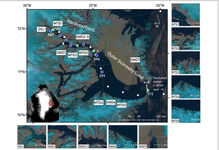
Scoresby Sund covers an area of 13,700 km2with a total distance of 350 km between the head of the inner fjord and the mouth (Figure 1). The adjacent continental shelf has a width of 80–
100 km until the shelf break.Lewis and Smith (2009)determined the average annual meltwater production in the climatic region of Scoresby Sund (which is about 5% of Greenland’s surface area) to be 8 km3, plus an unknown volume from a number of potential meltwater outlets that could not be confirmed by satellite images. This corresponds to 2% of the average annual meltwater production of all climatic regions of Greenland. The fjord itself is divided into separate parts: the wide outer fjord (hereafter named Outer Scoresby Sund, OSS) with a maximum depth of 650 m and a rather uniform bottom topography, as well as several narrower inner fjords. The inner fjord arms are characterized by complex bottom topography and steep slopes, with water depths of up to 1,500 m (Funder, 1972; Dowdeswell et al., 1993; Ó Cofaigh et al., 2001). This study is focused on the northernmost fjord arm, Nordvestfjord. Nordvestfjord has a total length of 140 km and a width of about 5 km.
Numerous smaller branches join this fjord (Dowdeswell et al.,
FIGURE 1 |Landsat 8 false color images (OLI/TIRS C1 Level-1, courtesy of the U.S. Geological Survey) of the period of sampling (15 to 26 July 2016, depending on image availability and cloud cover), showing the Scoresby Sund fjord system and the fjord parts visited, namely Nordvestfjord and Outer Scoresby Sund (OSS). Light blue regions correspond to the ice cover of the GrIS. Major marine-terminating glaciers (MTG1-5) and surface meltwater discharges (SMD1-7) are marked in the map and displayed in enlarged images. Daugaard-Jensen glacier (DGJ) is indicated at the head of Nordvestfjord. White lines at the fjord mouth (A+B) and the entrance to Nordvestfjord (C) mark the positions of the LADCP transects during MSM76. Marks show sampling stations during MSM56, with green pentagons showing where sediment traps were deployed, and blue pentagons indicating where the camera profiles were performed. At the other stations (white circles), the standard sampling program was conducted, including CTD casts and in most cases sampling for nutrients and dissolved inorganic carbon/total alkalinity. Station numbers are included for stations that are explicitly mentioned in the text. Note that some stations were visited twice, upon entering and exiting the fjord system.
2016) which is separated from the OSS by a sill having a depth of<350 m.
Daugaard-Jensen glacier at Nordvestfjord’s head is a prominent marine-terminating glacier and the main generator of icebergs (Ó Cofaigh et al., 2001). The closest hydrographic station to the glacier terminus was situated 8–10 km away.
Other large marine-terminating glaciers as well as major surface meltwater runoff pathways were identified by visual inspection of Landsat satellite images (USGS, EarthExplorer, Landsat 8 OLI/TIRS C1 Level-1, Figure 1) collected during our occupation of the fjord. In addition to Daugaard- Jensen glacier, three marine-terminating glaciers drain into Nordvestfjord and two into the OSS, with front widths of 1–11 km. Seven meltwater rivers flow into Nordvestfjord and two into the OSS.
2.2. Sample Collection and Analysis
Data were collected during a comprehensive sampling program with the German research vesselRV Maria S. Merian (cruise MSM56) (Koch, 2016). Twenty-two stations were sampled between 10 and 19 July 2016 along a transect from the inner Nordvestfjord to the fjord mouth, and additional three stations at the Greenland shelf (Figure 1).
At each station a CTD (Conductivity-Temperature-Depth) probe (SBE11plus Deck Unit with SBE9 sensors, Sea-Bird Scientific) equipped with additional sensors recorded vertical profiles of temperature, salinity, turbidity (ECO-NTU, WET Labs, Sea-Bird Scientific), chlorophyll a fluorescence (ECO- AFL/FL, WET Labs, Sea-Bird Scientific), and dissolved oxygen (SBE43, Sea-Bird Scientific) (Friedrichs et al., 2017). If not denoted differently, we reportin situtemperatures in◦C. Water
samples were drawn from a rosette sampler with 24 Niskin bottles from discrete depths during the up-cast. Dissolved oxygen samples were taken for sensor calibration at all stations, and measured onboard within 24 h using Winkler titration. Salinity samples were collected in glass bottles and measured in the home laboratory. Note that all salinities in this paper are given on practical salinity scale (determined by electrical conductivity of seawater). Samples for nutrients (phosphate, nitrate, silicate) were collected in 50 ml LDPE bottles and stored frozen until analysis in the home laboratory. Nutrient concentrations were determined by a spectrophotometric autoanalyzer (QuAAtro39, SEAL Analytical) using slightly modified standard methods (Kattner and Becker, 1991). The measurement precision was 0.3% (coefficient of variation). Calibration of the nutrient analyses was performed using certified reference material (NMIJ CRM 7602-a, Seawater for Nutrients, National Metrology Institute of Japan, Ibaraki, Japan). Water samples for the determination of dissolved inorganic carbon (DIC) and total alkalinity (TA) were collected in 300 ml borosilicate bottles, poisoned with mercuric chloride, sealed, and stored in a cool place and in the dark. Measurements of DIC and TA were conducted with a VINDTA 3C (Versatile INstrument for the Determination ofTotal inorganic carbon and titrationAlkalinity, Marianda, Kiel) including a CO2 coulometer CM5015 (UIC Inc.) in the home laboratory. DIC was determined at 10◦C by coulometry (Johnson et al., 1993; Dickson et al., 2007) with a precision of 1.4µmol kg−1. TA was measured at 25◦C by applying a Gran potentiometric titration (Gran, 1952) with a precision of 1.8µmol kg−1. The methods were calibrated using certified reference material (batches #102 and #161) supplied by Scripps Institution of Oceanography, USA.
We used free-drifting surface tethered sediment traps to measure export flux at 100, 200, and 400 m depth for 5–10 h (Figure 1). The drifting traps consisted of a single drifting array with a surface buoy equipped with a GPS satellite transmitter, 12 small buoyancy balls serving as wave breakers to reduce the hydrodynamic effects on the sediment traps, and two 25 l glass buoyancy spheres. Each collection depth had four gimbal mounted collection cylinders, each 1 m tall and 10.4 cm in inner diameter. The collection cylinders were filled with filtered sea water with slightly increased salinity (4 permille increase) before deployment. The collected material was fixed with mercuric chloride and stored at 4◦C until further analyses in the home laboratory. For the determination of the POC flux at the trap depths, samples were filtered on pre-combusted (450◦C, 12 h) and pre-weighted Whatman GF/F filters (diameter: 25 mm) after removing swimmers, and dried for 48 h at 50◦C. To remove particulate inorganic carbon, filters were fumed with 37% fuming hydrochloric acid for 24 h, dried for 24 h, and analyzed with a gas chromatograph (GC) elemental analyzer (EURO EA). In order to obtain discrete estimates of the POC flux in g C m−2d−1at the depths of the trap deployments, the weight of POC in a sample was divided by the area of the trap opening and the deployment time of the traps. For the determination of continuous POC flux profiles based on the discrete POC flux estimates of the sediment traps, we conducted optical recordings of vertical profiles at 12 stations using an in situ camera system (Figure 1). The
custom camera system was self-constructed at AWI/MARUM and equipped with an infrared camera (acA2010-25gc GigE camera, Basler), an Edmund Optics compact fixed focal length lens 25 mm (#67-715) with aperture F#16, and an infrared light source. Every 500 ms (equivalent to a 15 cm depth interval), one picture was taken covering a volume of 20.46 cm3. The pictures were analyzed for particle size distribution and abundance by image processing using the image processing toolbox in Matlab R2015a (The MathWorks, Inc., Natick, MA, USA), following the method of Iversen et al. (2010)(see section 2.3). POC fluxes obtained from sediment trap deployments were used to fit the particle masses and sinking velocities (Iversen et al., 2010).
A HyperPro II profiling system (Satlantic, Canada) was used to acquire underwater light field information at selected stations depending on sea, weather, and daylight conditions, following procedures from Holinde and Zielinski (2016). Hyperspectral Ed(λ) data were then processed with ProSoft v.7.7.16 (Satlantic) and binned to 1 m depth intervals to calculate photosynthetically active radiation (PAR). Based on PAR(z), the 1% depth of PAR (a common indicator for the depth of the euphotic zone) was derived followingRichlen et al. (2016), where PAR(0 m) data was extrapolated from the top 5 measurements.
In order to put the observed hydrographic and biogeochemical distributions into the context of ocean circulation, we analyzed direct velocity observations. Because they were not available from the cruise MSM56 in summer 2016, we use data that were obtained during theRV Maria S. Merian expedition MSM76 in summer 2018. This cruise was later in the year (11 August to 11 September 2018), but we believe that summer conditions, including the melting of marine- and land-terminating glaciers, led to similar circulation patterns as during the cruise MSM56 2 years earlier. Two meridional CTD and LADCP sections were carried out across the mouth of Scoresby Sound (sections A and B; see sectionFigure 1) from coast-to-coast, each comprising six stations. The work on section A started in the late afternoon, while section B was occupied 30 h later. Both sections were accomplished within roughly 7 h. In addition, one section consisting of four stations was carried out from coast-to-coast across the transition between the OSS and Nordvestfjord (section C; seeFigure 1).
Regarding marine-terminating glaciers, the resolution of our dataset does not allow to distinguish between subglacial discharge (surface melt that is discharged through channels at the glacier base) and submarine melt (meltwater from below sea level) (Straneo and Cenedese, 2015). We therefore use both terms synonymously, even if we are aware that both meltwater types might enter the fjord waters in different ways.
2.3. Data Compilation
To assess the productivity of the fjord system, we calculated the net community production (NCP), which is defined as the gross primary production minus all losses in carbon due to respiration.
It is used as a measure for the fraction of primary production that will be exported out of the surface layer, i.e., export production (Williams, 1993; Hansell and Carlson, 1998; Lee, 2001). NCP quantifies all biological activity that has occurred since ice break- up in spring until the time of sampling. While there are different
methods to determine NCP (e.g., Hansell and Carlson, 1998;
Bates et al., 2005; Munro et al., 2015), we utilize the difference in nutrients (particularly nitrate+nitrite and phosphate) between the winter and the time of sampling (Hoppema et al., 2007;
Ulfsbo et al., 2014). In the high-latitude oceans and thus also in fjords, a remnant layer from the previous winter occurs below the seasonally heated surface layer. In this layer, nutrient concentrations are found as in winter (though sampled in summer). The winter remnant layer is defined by a temperature minimum below the seasonal halocline, and therefore kept out of contact with the atmosphere (Rudels et al., 1996; Hoppema et al., 2000, 2007; Ulfsbo et al., 2014). Because local vertical mixing had modified the temperature minimum to some extent, resulting in variability of the nutrient concentrations, we used the mean nutrient concentration of the Polar Water on the shelf (see definition of this water mass in section 3); here we assume that this is the main subsurface water source to the fjord and its residence time is more than 1 year. The temperature and salinity sections (Figures 4A,B) appear to confirm the Polar Water to be this source. Mean concentrations in the Polar Water at three shelf stations were 6.3±1.3µmol l−1 for nitrate+nitrite, and 0.6± 0.09µmol l−1for phosphate. For the depth of the winter remnant layer we took the temperature minima at the individual stations (between 41 and 135 m depth).
The net nutrient drawdown was obtained at each station by integrating the difference between the concentration in the temperature minimum and that in the surface layer above it.
To exclude dilution by ice melt, evaporation, and precipitation, nutrient concentrations were normalized to a constant salinity of 34.5, as described inHoppema et al. (2007). We then applied the following equation (modified afterUlfsbo et al., 2014):
NCPx[mmol C m−2period−1]= ZTmin
0 (Xinitial−Xmeasured)dz·RC/X, (1) whereXrepresents the nutrient concentration, either initial in the winter remnant layer, or measured at each sampling depth.
RC/X is the stoichiometric nutrient ratio which is necessary to convert nutrient units to carbon units. In this study we use the canonical Redfield ratio of 106C:16N:1P (Redfield et al., 1963).
The integration was performed by linear interpolations between nearest sampling depths. In Young Sound, primary production below sea-ice was negligible because of a thick snow cover and active sea-ice melt which limited sea-ice-related production rates to 1 month or less (Glud et al., 2007). Based on this, we assumed that biological production in Scoresby Sund started with ice break-up (which we identified using satellite images), and could then calculate the daily NCP. The dates of ice break-up, the number of open water days until sampling, and the NCP based on nitrate+nitrite and phosphate deficits at each station are listed in Table 1. Upwelling of nutrients from depth can result in an underestimation of the NCP. However, upwelling during summer in Scoresby Sund does not fuel the whole surface layer (see section 4.2.1). Hence, we believe that it does not severely affect primary production and, thus, the production
estimate based on nutrient deficits. NCP estimates can fluctuate depending on the assumptions made during the computation process. The main assumptions in the calculation of NCP are:
(1) The source water is the Polar Water from the shelf near the mouth of Scoresby Sund; the source concentrations of nutrients may have been changed during transfer through the fjord system, both laterally and vertically. Since the Polar Water is vertically separated from its neighboring water masses by strong gradients, little exchange will likely occur with these during its transfer through the fjord. For the same reason, the vertical exchange at the stations is thought to be relatively small. (2) Homogeneity of the water column during winter and negligible winter draw- down of nutrients; in other fjords, winter draw-down has been observed, although not in all fjords (Glud et al., 2007); this may lead to a slight underestimation of the computed NCP.
Accounting for variability in our definition of winter nutrient concentrations resulted in deviations in our estimates of NCP of
±18% (from nitrate+nitrite deficits) and±41% (from phosphate deficits) from the ones presented here.
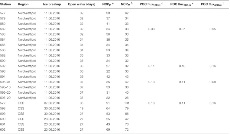
Figure 2presents the total aggregate volume and the POC flux throughout the water column as estimated from camera images.
In the following, we use the term “particles" to refer to aggregates of inorganic and dead organic material and fecal pellets, while the POC flux only comprises the mass flux of organic carbon that is incorporated in the particles. Particle abundance and size were recognized using an image analyzing tool (medfilt2 function in Matlab R2015a) after converting the pictures into binary files and correcting them for background disturbance, such as shadows from illumination artifacts and spots on the camera lens. The pixel number of each projected particle area was determined and converted into equivalent spherical diameter (ESD) using the pixel to mm ratio. Detected particles were sorted into 20 logarithmically spaced size bins (d) based on their ESDs, ranging from 20 to 3415.03µm. Each picture was concatenated to its respectivein situdepth. Knowing the volume of the water cell pictured by the camera, the number of particles per liter and size class could be calculated (1C), and from it the total particle volume (Figure 2A). To account for statistical relevance, especially for the sparse large particles, we binned 10 consecutive pictures and only included size bins that contained five or more aggregates. In order to calculate the particle size distributionn, the number of particles per liter in a given size class was divided by the size difference between the concomitant size classes, as described by Iversen et al. (2010). As the POC flux within a certain time period was estimated from sediment traps that were deployed at three depths in the water column, a time dimension and POC estimate could be given to the particle volume (Figure 2B). For this, the total POC fluxFwas assumed to be an integration of the mass flux spectra of all particle sizes (modified afterIversen et al., 2010):
F=
Z size class20 size class1
n(d)·m(d)·w(d)·d(d), (2)
wheren(#m−3cm−1) is the particle size distribution in a given small size range,d(d), mis the particle mass (as POC), andw (m d−1) is the average sinking velocity of the particles in a given
TABLE 1 |Time of ice breakup, NCP (based on nitrate+nitrite, and phosphate), and flux of particulate organic carbon measured in sediment trap samples per station (stations with only CTD and shelf stations casts are not included). At station 595, four sampling rounds were conducted within 24 h.
Station Region Ice breakup Open water (days) NCPPa NCPNb POC flux100mc POC flux200mc POC flux400mc
577 Nordvestfjord 11.06.2016 32 30 62
579 Nordvestfjord 11.06.2016 32 37 34
580 Nordvestfjord 11.06.2016 32 41 33
582 Nordvestfjord 11.06.2016 32 34 33 0.33 0.37 0.55
583 Nordvestfjord 11.06.2016 32 36 33
584 Nordvestfjord 11.06.2016 34 36 35
585 Nordvestfjord 11.06.2016 34 34 34
586 Nordvestfjord 11.06.2016 34 33 34
588 Nordvestfjord 11.06.2016 35 33 33
590 Nordvestfjord 11.06.2016 35 24 32
592 Nordvestfjord 11.06.2016 35 27 32 0.11 0.10 0.16
593 Nordvestfjord 11.06.2016 36 22 33
594 Nordvestfjord 11.06.2016 36 42 43
595–01 Nordvestfjord 11.06.2016 37 35 42 0.13 0.11 0.08
595–10 Nordvestfjord 11.06.2016 37 33 38
595–20 Nordvestfjord 11.06.2016 37 31 40
595–29 Nordvestfjord 11.06.2016 37 22 25
572 OSS 07.06.2016 35 91 101 0.13 0.11 0.16
598 OSS 30.06.2016 19 64 79
599 OSS 30.06.2016 27 53 68
600 OSS 23.06.2016 27 25 42
601 OSS 23.06.2016 27 43 70
602 OSS 23.06.2016 27 69 72
acalculated based on phosphate deficits, in mmol C m−2d−1. bcalculated based on nitrate+nitrite deficits, in mmol C m−2d−1. cin g C m−2d−1.
small size range,d(d). Whilenanddare known,mandwhave to be determined. Since both particle massmand sinking velocity wscales as a power relationship when expressed as a function of particle diameterd, the product ofm andwalso scale as a power relationship as a function ofd. We used a minimization procedure to find the factor and exponent providing the best- fit between the trap collected fluxes and F obtained from the in-situ images at the trap depths, using the Matlab R2015a functionfminsearch.
As most of the camera profiles did not cover the water column down to the bottom, we fitted a Martin curve to the profiles for extrapolation (Martin et al., 1987; Belcher et al., 2016):
F(z)=F(z0)·(z/z0)−b, (3) where F is the POC flux at depths z0 and z, and b is the remineralization exponent. This exponent can also be considered as efficiency with which carbon that is exported from the upper ocean, i.e.,F(z0), decreases with depth (Guidi et al., 2015). Highb values indicate high degradation of organic matter, while negative b values show initially increasing POC flux with depth. From the camera profiles we obtained a b value for each station.
By replacing F(z0) by the NCP at each station and using the correspondingbvalue, the fraction of NCP potentially reaching the sea floor was determined (Figure 2B).
The Martin curves differ considerably from the POC flux profiles at the surface, which might be the result of small particles that could not be detected on the images. However, the general pattern of the decrease in POC flux is consistent: POC flux and total aggregate volume peak in the upper 100 m of the water column, and particles are attenuated to low and quasi constant fluxes at depths below 200 m. To test the robustness of the findings based on thebvalue with a more simple approximation of export and remineralization, we calculated the ratio between the discrete POC fluxes at 100 m depth and the NCP estimates at the camera stations (by relating sediment trap stations with the closest camera stations).
3. RESULTS
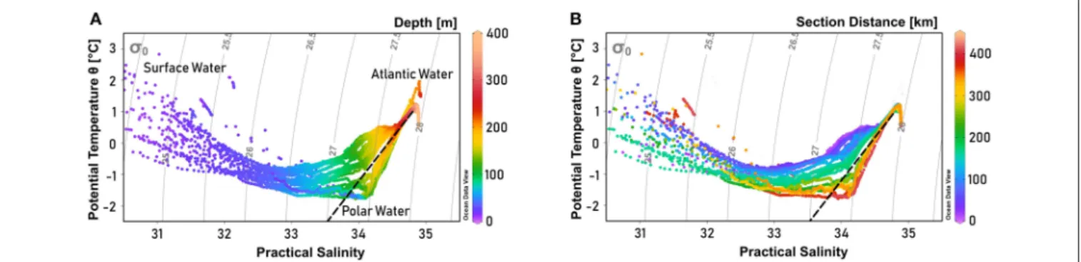
On the shelf of east Greenland, Polar Water (PW) with a salinity (S) below 34, and temperature (T) near the surface freezing point—exported from the Arctic Ocean—is advected toward the south near the sea surface. Below the PW, a warm and saline water mass (T>0◦C) is found, referred to as Atlantic Water (AW). A warmer and more saline variety of AW originates from waters recirculating in Fram Strait, while a slightly colder and fresher AW type is exported from the Arctic Ocean (Rudels
FIGURE 2 |Vertical distribution of the(A)total particle volume [cm3l−1], and (B)POC flux [g C m2d−1]. An artifact on a picture at 100 m depth lead to a single high value in(A), but by relating the sediment trap POC measure during the computation process to all pictures within a depth range of 10 m above and below the actual depth of the sediment trap, this artifact was removed in (B). The dotted line in(B)indicates the Martin curve based on the maximum and the deepest POC fluxes. For the dashed line in(B), the remineralization exponentbfrom the previous fitting as well as the NCP at the surface were used.
et al., 2002). The characteristics of PW and AW are well- reflected by the water masses in OSS (Figures 3A,4A,B), with PW found approximately above 200 m. Specifically, pronounced PW properties with temperatures below -1.4◦C are observed at depths shallower than 150 m. Within the AW layer, found approximately below 200 m, salinity increases toward the bottom, while there is a temperature maximum near 1.2◦C well-above the sea floor and a temperature minimum of T<0.7◦C at the bottom (Figures 4A,B). In addition, above the PW a ∼10 m thick very fresh surface layer was recorded, with temperatures sometimes exceeding 3◦C, most likely reflecting summertime surface discharge of meltwater from the GrIS combined with solar heating in the fjord. As a result, maximum mixed layer depths are limited to the upper 10 m of the water column. During the cruise we noticed the presence of icebergs from calving glaciers in the whole fjord with increasing density toward the fjord head.
Hydrographic properties change along the fjord axis from the mouth toward the inner part of Nordvestfjord. At depths below 400 m, the entire Nordvestfjord is filled by AW with temperatures exceeding 1.1◦C (Figure 4A). This indicates that the sill separating the OSS and Nordvestfjord only allows for the warmer and less dense AW fraction to flow from the OSS into Nordvestfjord, while the colder AW bottom layer is held back. While the AW temperature maximum remains largely unchanged throughout the fjord system all the way into inner Nordvestfjord, the subsurface waters above the AW layer
experience substantial warming with increasing distance from the mouth. As can be seen fromFigures 3A,5A,Btemperatures are higher than –1.0◦C in this layer in Nordvestfjord, even up to 0.5◦C. Consequently, the steep transition in T/S space from PW to the AW temperature maximum present at the mouth of Scoresby Sound is observed to level off toward the inner fjord with the sill toward Nordvestfjord marking at particularly pronounced transition in T/S space around the 27.5 kg m−3 isopycnal (Figure 3B). At the same time, the 27.9 kg m−3isopycnal deepens from 300 m in the OSS to 500 m in Nordvestfjord, indicating higher densities (salinities) to be present in the OSS compared to Nordvestfjord in this depth range. This pattern is reminiscent of a deep overflow (spill) of AW across the sill that, however, does not extend all the way to the bottom in Nordvestfjord.
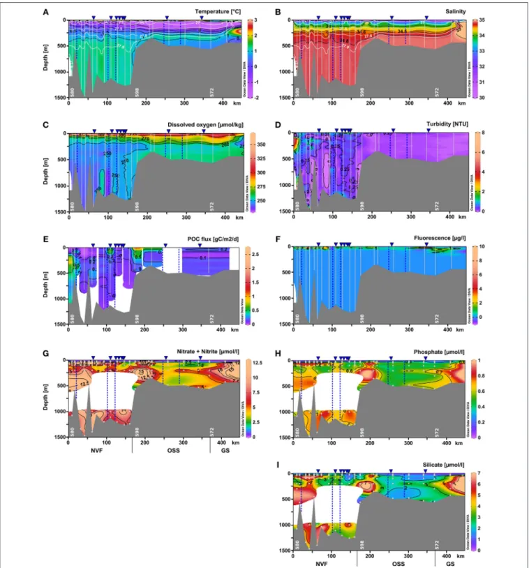
Dissolved oxygen concentrations were lowest in the deep basin (>700 m), reaching ∼240µmol kg−1. In Nordvestfjord between 10 and 30 m depth, the highest dissolved oxygen concentrations were found reaching 350µmol kg−1 and in the OSS in the same depth range these values decreased to 320µmol kg−1. In the upper 10 m of the water column of the OSS, dissolved oxygen concentrations were much lower reaching 280µmol kg−1, but increased to 300µmol kg−1toward the fjord mouth (Figures 4C,5C).
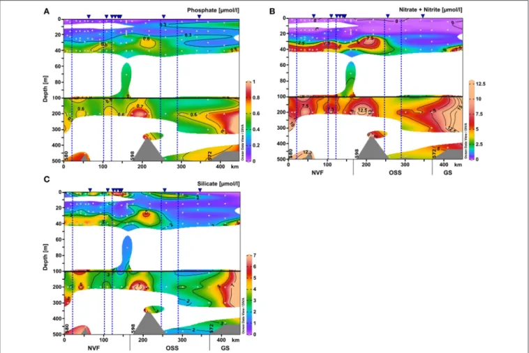
The surface water nutrients in the upper 25 to 50 m were largely depleted, with concentrations of about 0.1, 0.2, and 1.2µmol l−1 for nitrate+nitrite, phosphate, and silicate, respectively (Figure 6). An exception was a region at 120–
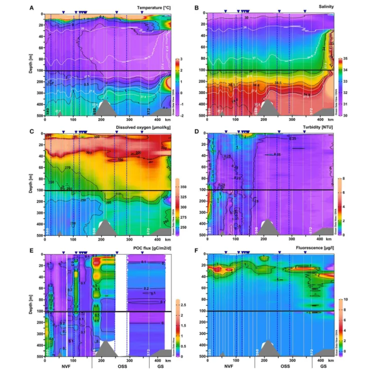
150 km section distance characterized by high surface meltwater discharge (Figure 1, SMD2-5) where silicate concentrations reached up to 6.0–6.1µmol l−1, which is 2–3 times higher than in the surface layer at all other stations (Figure 6C). No other nutrient had such elevated concentrations here and also chlorophyllafluorescence did not show a maximum. Between 20 and 30 m depth, chlorophyll a fluorescence was high with maximum values of up to 6.6µg l−1 at the innermost stations (0–100 km section distance), but decreased considerably to about 1.4µg l−1 at a section distance of 100 km and further toward the transition to the OSS (Figures 4Fand5F). Beneath 30 m depth, nutrient concentrations were significant but not homogeneously high within the water column of Nordvestfjord.
The OSS was supplied by nutrients from the Greenland shelf that were transported within PW and AW at depths from 40 m to the bottom with concentrations of up to 12µmol l−1 for nitrate+nitrite, 0.8µmol l−1for phosphate, and 6.0µmol l−1 for silicate. These concentrations decreased toward the sill to Nordvestfjord (Figures 4G–I). Chlorophyll a fluorescence was high with maximum values of 9.8µg l−1within a layer at 25–50 m depth (Figure 5F).
Two patches of high chlorophyllafluorescence in the OSS with 1.2 and 9.8µg l−1correlated with patches of high dissolved oxygen concentrations (301.5 and 302.4µmol kg−1) and high turbidity (0.14 and 0.35 NTU) at 46 and 27 m depth and 260 and 300–340 km section distance, respectively (Figures 5C,D,F).
Otherwise, turbidity was low in the OSS with about 0.09 NTU compared to Nordvestfjord with 0.3–0.5 NTU and a throughout turbid water column (Figure 4D). Highest turbidity in the
FIGURE 3 |Temperature-salinity diagram of Scoresby Sund, showing the primary water masses present in the study area (afterRudels et al., 2002). Colors indicate (A)depth and(B)section distance, while gray lines indicate isopycnals. The dashed black line represents the Gade line between the Atlantic Water (T = 1◦C, S = 34.8) and the meltwater endmember of glacier termini (T = –90◦C, S = 0). One station with a distinct Atlantic Water signal was not included in the section profiles, as it was further north on the Greenland shelf. It is therefore visible in(A), but not in(B). Potential temperature was derived fromin situtemperature using Ocean Data View 4 software (Schlitzer, 2004).
Nordvestfjord was found at 100–200 m depth at the station closest to Daugaard-Jensen glacier, with a maximum of 3.8 NTU at 120 m depth (Figure 5D). Besides, values close to the surface and to the bottom were elevated with 0.6–0.7 and 0.5–0.8 NTU, respectively. At 120–150 km section distance, surface turbidity was almost one order of magnitude higher than within large parts of the water column (2.2–2.9 NTU), coinciding with elevated silicate concentrations (Figures 5D,6C).
The depth of the euphotic zone as derived from the 1%
depth of PAR ranged between 20 and 69 m throughout the whole study area. While light penetration varied in the Nordvestfjord between 20 and 44 m (mean = 32 m, standard deviation = 7 m), it increased toward the OSS and the adjacent Greenland shelf, ranging from 34 to 69 m (mean = 48 m, standard deviation = 11 m).
DIC and TA correlate strongly with salinity (R2DIC = 0.906 and R2TA = 0.942; n = 54 for DIC, n = 46 for TA) (Figures 7A,C). Normalization to a constant salinity of 34.5 revealed that low-salinity samples (mainly surface samples of Nordvestfjord) were profoundly affected by processes other than dilution (Figures 7B,D). They were therefore not taken into account for the extrapolation to zero salinity (i.e., representing meltwater discharge), which yields concentrations of 423 and 726µmol kg−1 for DIC and TA, respectively (Figures 7A,C).
Note that these freshwater endmember concentrations were used for salinity normalization (Friis et al., 2003), but that assuming a freshwater endmember with zero concentrations of DIC and TA, respectively, resulted in the same trend for normalized low-salinity samples. Non-conservative changes in DIC can be caused by a number of processes, including uptake of atmospheric CO2, remineralization, and photosynthesis. No clear trend could be identified in the normalized DIC values of low- salinity surface samples (Figure 7B), indicating an interaction of several processes. Non-conservative behavior of TA, by contrast, is mainly attributed to carbonate mineral precipitation and dissolution (e.g.,Cross et al., 2013). As most low-salinity surface samples had lower normalized TA values than the samples with higher salinities (which display a conservative relationship
between TA concentration and salinity) (Figure 7D), we assume that they reflect carbonate mineral precipitation.
The NCP was high in the OSS (58 mmol C m−2d−1 for phosphate deficits, 82 mmol C m−2d−1 for nitrate+nitrite deficits) compared to Nordvestfjord (32 mmol C m−2d−1 for phosphate deficits, 36 mmol C m−2d−1 for nitrate+nitrite deficits; Table 2). Visual analyses of net samples from Nordvestfjord revealed that the phytoplankton community was already in a post-bloom stage (B. Edvardsen, personal communication). Much debris, many copepods, and fecal pellets found in the sediment traps show that intense grazing already diminished the primary production. By contrast, a healthy and thriving phytoplankton community was observed in net samples of the OSS.
Camera-derived POC fluxes in Nordvestfjord and at the innermost part of OSS were high close to glacier fronts, ranging from 0.5–2 g C m−2d−1, and lower in the remaining Nordvestfjord (0.1–0.3 g C m−2d−1;Figure 4E). In the OSS, they decreased with increasing depth within the surface layer and corresponded well with the stratification of the water masses below (0.1–0.2 g C m−2d−1). It has to be noted that only one POC flux profile is available for the OSS and none for the shelf.
Thebvalue, constituting the remineralization efficiency, is higher in the OSS (0.3–0.4) than in Nordvestfjord (–0.4–0.6), indicating that a smaller share of the surface production in the OSS is transported to depth. The POC100m : NCP ratio confirms this, showing that the POC flux at the depth of the shallowest sediment trap at 100 m makes up only 10–20 or 10–30% (for NCPNand NCPP, respectively) of the surface production in the OSS, while in Nordvestfjord, 30–80% of the NCP (both, NCPNand NCPP) are reflected in the POC flux at 100 m depth. According to the Martin curve, between 0.06 and 2.5 g C m−2d−1of POC reached the sea floor in Nordvestfjord, which is more than the average amount fixed per day by primary production since the start of the growing season, whereas only 5–15% of the NCP in the OSS was sedimented on the seafloor (0.1–0.2 g C m−2d−1) (Table 2).
Traces of the pronounced freshwater discharge of Daugaard- Jensen glacier were detectable 8-10 km away from the glacier
FIGURE 4 |Vertical distribution of(A)temperature (◦C),(B)salinity,(C)dissolved oxygen (µmol kg−1),(D)turbidity (NTU),(E)POC flux (g C m−2d−1),(F)chlorophyll afluorescence (µg l−1),(G)nitrate+nitrite (µmol l−1),(H)phosphate (µmol l−1), and(I)silicate (µmol l−1) as distance from the fjord head (left) to the shelf (right) using Ocean Data View 4 software (Schlitzer, 2004). Data were interpolated by DIVA gridding, or for the POC fluxes by weighted-average gridding due to the low profile number. Bright lines indicate the CTD and camera profiles, bright dots represent water samples. The approximate positions of marine-terminating glaciers are shown by blue dashed lines, and surface meltwater discharge by blue triangles above the panels. Daugaard-Jensen glacier is situated close to the westernmost station (left side of the panels). NVF is the acronym for Nordvestfjord, OSS stands for the Outer Scoresby Sund, and GS for the Greenland Shelf.
FIGURE 5 |Same asFigure 4for the upper 500 m of the water column:(A)temperature (◦C),(B)salinity,(C)dissolved oxygen (µmol kg-1),(D)turbidity (NTU),(E) POC flux (g C m-2 d-1), and(F)chlorophyll a fluorescence (µg l-1). Section plots of the nutrient distributions are inFigure 6. The scale of the upper 100 m was expanded.
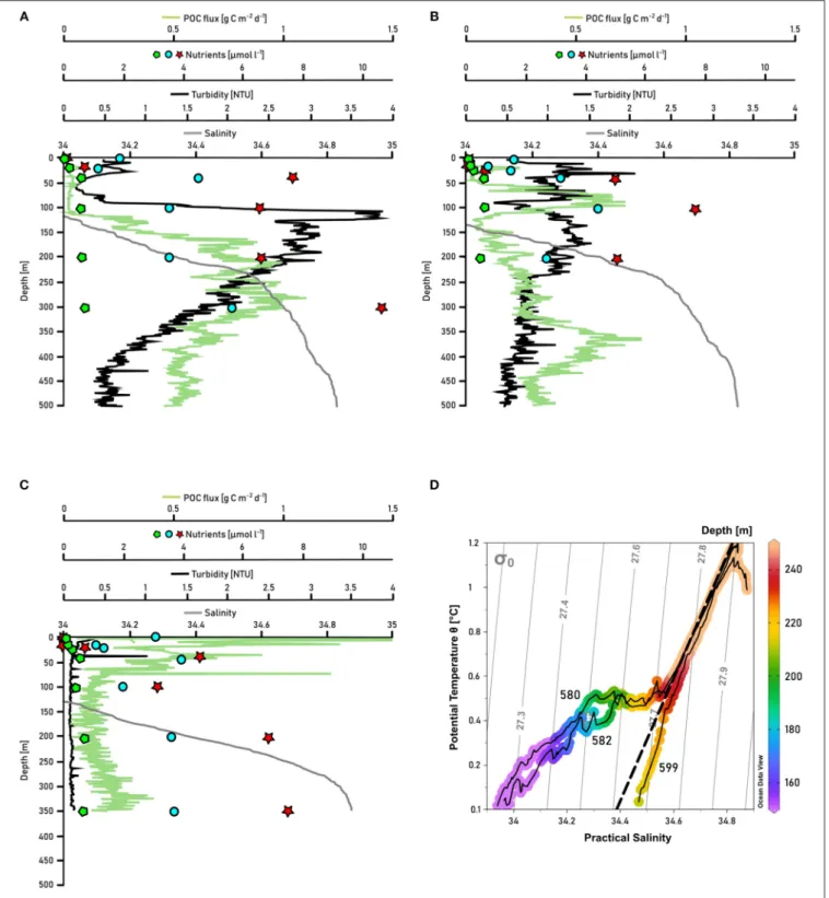
front at our station closest to the terminus (station 580). In order to highlight the impact of Daugaard-Jensen’s meltwater discharge on biogeochemical cycling in Scoresby Sund, we contrast measurements at two other stations (station 582 which is∼7 km further north of station 580, and station 599 in the OSS) in the same way as for station 580 (Figure 8). While at other stations at 200–240 m depth, salinity smoothly decreased with
depth (examples given inFigures 8B,C), a sudden salinity drop by 0.1–0.2 units could be detected at station 580 (Figure 8A).
The temperature-salinity diagram reveals a salinity-driven density decrease, indicated by an approximately horizontal line compared to the stations 582 and 599 (Figure 8D). At station 580, nutrient concentrations were reduced by one third at 100–200 m depth compared to nutrient concentrations at
FIGURE 6 |Same asFigure 4for the nutrient distributions within upper 500 m of the water column:(A)nitrate+nitrite (µmol l-1),(B)phosphate (µmol l-1), and(C) silicate (µmol l-1). The scale of the upper 100 m was expanded.
300 m depth. At 40–100 m depth nutrient concentrations were slightly higher. A reversed pattern was observed for turbidity, with a maximum at 100–200 m depth (2.5–3.9 NTU) and lower turbidity in the water masses above 100 m and below 200–
250 m at this station. NCP, reaching 41 and 33 mmol C m−2d−1 (for phosphate and nitrate+nitrite deficits, respectively), was not considerably higher compared to NCP at other stations (Table 1), but the POC flux was elevated at 250–350 m depth (up to 1 g C m−2 d−1) and with 4.0–4.9 g C m−2d−1(bvalue: -0.57) the sedimentation rate to the bottom was higher next to the glacier (station 580) than in the remaining Nordvestfjord. Maximum nutrient concentrations at the next station further outfjord (station 582) were measured at 100 m depth, coinciding with a POC flux maximum of 0.8 g C m−2 d−1. Turbidity was higher within the upper 250 m (∼1 NTU) than below (∼0.5 NTU).
At a station within the shallower OSS (station 599), nutrient concentrations were increasing from the surface up to a depth of 50 m, which coincides with an elevated POC flux (up to 0.4 g C m−2d−1), high turbidity (1.5–3.0 NTU), and high chlorophyllafluorescence (Figure 5F), indicating active primary production and remineralization. Below, nutrient concentrations and turbidity increased toward the depth of the AW (200 m), while the POC flux stayed low throughout the water column.
4. DISCUSSION
Figure 11summarizes the main processes that are discussed in the following chapters.
4.1. Circulation
The circulation of AW (i.e., temperatures exceeding 0◦C) at the fjord mouth (sections A and B; seeFigure 1) is characterized by an inflow of AW into Scoresby Sund at the northern part of the section and an outflow of AW in the southern part (Figure 9, upper panel). Thereby, the strongest flows are observed close to the northern and southern margins, suggesting boundary currents to be present along either margins. The observed circulation in the PW layer is considerably more patchy and weak overall (Figure 9, upper panel). In order to quantify the strength of the circulation, cumulative cross-section transports (integrated from north to south) have been computed for both sections A and B (Figure 9, lower panel). This has been done both based on the observed velocities (solid lines) and after a correction for barotropic tidal currents was applied (dashed lines). Despite differences between the 4 graphs, there is qualitative agreement in the sense that the inflow is found in the northern half of the section and outflow in the southern
FIGURE 7 |Least-square linear regressions of(A)Total dissolved inorganic carbon (DIC) vs. salinity (R2= 0.906) and(C)Total alkalinity (TA) vs. salinity (R2= 0.942).
Linear regressions were performed based only on samples with salinities>25. Normalization of(B)DIC and(D)TA was performed according to the formula ofFriis et al. (2003)for non-zero freshwater endmembers. Dashed lines in(B,D)represent the approximate mean values of the samples with salinities>25. Deviations relative to this line (low-salinity samples, mainly from the surface of Nordvestfjord) indicate processes other than conservative mixing that modify TA and DIC concentrations.
TABLE 2 |Production, carbon flux, and remineralization in Nordvestfjord (NVF) and the Outer Scoresby Sund (OSS).
NVF OSS
NCPPa(mmol C m−2d−1) 32±6 58±23
NCPNb(mmol C m−2d−1) 36±8 82±32
POC100m: NCPP 0.3–0.8 0.1–0.3
POC100m: NCPN 0.3–0.8 0.1–0.2
bvalue –0.4 –0.6 0.3–0.4
POCbottom(g C m−2d−1) 0.06–2.5 0.1–0.2
All values are averaged for the respective region or were given as a range between maximum and minimum value. Because of the influence of the Daugaard-Jensen glacier, data from the closest station to the glacier were not included but instead discussed separately. The low number of profiles only allowed to give a range for POCbottomand thebvalue, which indicates the degradation efficiency of organic matter, with high values showing high degradation, and low values showing initially increasing POC flux with depth.
acalculated based on phosphate deficits.
bcalculated based on nitrate+nitrite deficits.
part. The maximum inflow lies between 110 and 190·103m3s−1 for the original data and reduces to values between 60 and 100·103m3s−1 after tidal correction (Figure 9, lower panel).
Note that after tidal corrections for both sections there is a higher degree of compensation between inflow and outflow than without the correction (Figure 9, lower panel). As mass should be approximately conserved on weekly and long time scales, the tidal correction seems to add to the plausibility of the results.
Section C across the transition between the OSS and Nordvestfjord (seeFigures 1,10, left panel) is divided into two 4 km-wide channels separated by an island in the middle. The location where the section was taken is placed beyond the sill (at a distance of∼180 km;Figure 4A) where the sea floor slopes downward into Nordvestfjord. Here, a pronounced, bottom intensified inflow of the warmest part of AW into Nordvestfjord at densities exceeding 27.9 kg m−3 (and T>1.1◦C) is found in both channels. This supports the fact that the deep part of Nordvestfjord is filled by AW with temperatures exceeding 1.0◦C (Figure 4A). The outflow is found in both channels to occur mainly at middepths confined to a layer bounded by the 27.9 kg m−3 at the bottom and the 0◦C isotherm (i.e., the AW-PW interface) at the top. At shallower depths, a weak flow toward the OSS is found. Overall, the flow across section C seems to vary strongly with depth, with an inflow of warm AW of 65·103m3s−1 at the bottom, compensated by an outflow of slightly colder AW. There is no indication of pronounced horizontal recirculation as was found at the mouth of Scoresby Sund.
In summary, our observations suggest the presence of boundary currents at the mouth of Scoresby Sund. At horizontal scales exceeding the baroclinic Rossby Radius of deformation, RD, the Coriolis force is expected to impact the circulation such that boundary currents exist. Based on the hydrographic profiles, we estimated RD to amount to 6 km (following Nurser and Bacon, 2014), both at the mouth of the OSS and near the sill
FIGURE 8 |Salinity (gray line), turbidity (black line), POC flux (green line), nitrate+nitrite concentrations (red stars), silicate concentration (blue dots), and phosphate concentration (green pentagons) in the upper 500 m of the water column of the stations(A)580, which is closest to the glacier front of Daugaard-Jensen glacier,(B) 582, which is next to 580, but a bit further outfjord, and(C)599, a station in the middle of OSS.(D)displays the temperature-salinity diagrams of the three stations, colormarked for depths. Gray lines indicate isopycnals, the dashed black line represents the Gade line between the Atlantic Water (T = 1◦C, S = 34.8) and the meltwater endmember of glacier termini (T = –90◦C, S = 0). Potential temperature was derived fromin situtemperature using Ocean Data View 4 software (Schlitzer, 2004).
toward Nordvestfjord. The OSS exhibits typical widths of 35 km and exceeds 25 km at the mouth. This means that a horizontal circulation patterns with boundary currents along either margin represents plausible features of the circulation which we expect to exist throughout the OSS. The sense of the circulation (inflow along the northern margin and outflow along the southern one) can be reconciled with the fact that the Coriolis force acts on the flow to the right relative to the flow direction. At the transition of the OSS to Nordvestfjord (Figure 10), where the fjord becomes narrow, no evidence for horizonal recirculations are found. Here the flow seems to vary mainly in the vertical - reminiscent of estuarine circulations with an inflow at depth and outflow above this.
The inflow of warm AW into Scoresby Sund at depth and the compensatory outflow at shallower levels means that the heat, salt, and mass need to be transported upward within Nordvestfjord. The gradual warming of the subsurface layer (erosion of PW layer) may be explained by this. The fact that the isohalines are essentially flat in the upper 200 m throughout the OSS and Nordvestfjord may mean that there is a balance between salt being mixed upward and the input of freshwater from marine terminating glaciers and icebergs into the subsurface waters of the fjord.
4.2. Opposing Biogeochemical Regimes in Nordvestfjord and Outer Scoresby Sund
4.2.1. Nutrients and Turbidity
While deep nutrient concentrations in Nordvestfjord were elevated, the surface layer (up to 25–40 m depth) exhibited low nutrient concentrations (Figures 4G–I). Chlorophyll a fluorescence showed a maximum within a layer at 20–30 m depth, with laterally decreasing values in this layer with distance to the fjord head (Figure 5F). A surface patch with high silicate concentrations and elevated turbidity was found at 120–150 km section distance where numerous meltwater rivers drain into the fjord (Figures 1, 5D, 6C). Since there was no patch of other high nutrients, and the chlorophyll a fluorescence was not elevated, the surface meltwater must have been the source of silicate and silt. We assume that surface meltwater rivers accumulated silicate during their way across the bedrock surface.
Previous studies are not consistent in the information about the nutrient content of GrIS meltwater. While silicate has indeed been found to be transported into the system by glacial meltwater (Meire et al., 2016a; Hawkings et al., 2017), the meltwater contribution to phosphate and nitrate is unclear. The GrIS has been suggested to be a nitrogen source to phytoplankton (Hawkings et al., 2015, 2016; Wadham et al., 2016; Lund-Hansen et al., 2018). A fraction of this nitrogen might, however, not be readily bioavailable because it is bound to particles (Hawkings et al., 2015, 2016).
The indirect impact of glacier meltwater discharge on the distribution of nutrients and the resulting productivity in the fjord depends on the meltwater source. Meire et al.
(2017) described two possible patterns: a fjord dominated by marine-terminating glaciers is likely to be productive because
of enhanced upwelling of nutrient-rich deep water induced by the deep meltwater plume (see also Kanna et al., 2018).
By contrast, a fjord that is dominated by land-terminating glaciers discharges meltwater directly into the surface layer and is therefore characterized by low productivity because of enhanced stratification.
Nordvestfjord is influenced by both marine- and land- terminating glaciers. A third pattern besides the two described above seems to emerge here. Surface meltwater discharged into the fjord has formed a stable low-saline layer in the upper 10 m of the water column and below that the salinity increased only gradually. Also upwelling of nutrients due to meltwater release at greater depths seems to occur. Nutrient concentrations were high below 25–40 m depth, depending on the region. However, apparently they did not reach the surface layer above that.
Because of the low surface layer chlorophylla fluorescence at most stations, it is unlikely that such nutrients would have been consumed by primary production in the upper 10–25 m. While it appears that primary productivity in the innermost part of Nordvestfjord was still active, low chlorophyll a fluorescence values at stations further out (>100 km section distance until the sill to the OSS) suggest a termination of the bloom. The latter is supported by observations of a post-bloom plankton community, many copepods and fecal pellets in net samples and sediment traps during our cruise. Critical whether meltwater plumes of marine-terminating glaciers reach the surface or not are the distance to the glacier termini, the strength of the ambient stratification, the volume of subglacial discharge, and the grounding line depths (Sciascia et al., 2013; Carroll et al., 2015;
Hopwood et al., 2018). Even when not much is known about the marine-terminating glaciers in Scoresby Sund, it seems as if these factors produced plumes that obtained neutral buoyancy below the photic zone with only having a minor fertilizing effect on primary production. The depth of neutral buoyancy can be different for each marine-terminating glacier.
Within PW and AW, nutrients were transferred from the Greenland shelf to the OSS in the layer from 40 m to the bottom with concentrations of up to 12µmol l−1 of nitrate+nitrite;
0.8µmol l−1of phosphate; and 6.0µmol l−1of silicate. It seems as if these waters would not supply the whole Scoresby Sund with nutrients, because nutrient concentrations decrease shortly after entering the OSS. However, our stations were located at the southern side of the OSS entrance, and thus in the outflowing water (see section 4.1). If we would have sampled further north, the connection between the inner fjord waters and the shelf waters in terms of nutrient concentrations would possibly have been clear.
Above, we discussed why no nutrients arrived in the very surface layer (upper 10–20 m), resulting in a low primary productivity in Nordvestfjord. However, the situation with the nutrients supply to the euphotic zone is more complicated than this. The euphotic zone ranged from 20 to 44 m (see section 3). In a similar depth range of 20–35 m, the chlorophyllafluorescence maxima were found (Figure 5F). Nutrient concentrations were clearly higher in the deeper waters (>30 m) than in the near- surface water. This constellation can be explained by upwelling of nutrients which are consumed by primary producers near
FIGURE 9 |The(Upper panel)displays the across-section velocity profiles (vertical, dotted lines) (interpolated onto a regular grid using 2D-spline interpolation) along the mouth of Scoresby Sund as a function of both depth and along-section distance from northern section end point. The view is out-fjord directed. Blue shading denotes inflow of waters from the continental shelf into Scoresby Sund, while red shading denotes outflow. Also shown are selected isopycnals and isotherms as black and gray solid lines, respectively. The(Lower panel)displays the cumulative volume transport into Scoresby Sund (precisely, the meridional integral of the vertically integrated across-section velocity along the mouth of Scoresby Sund) as a function of along-section distance from the northern section end point. The transports based on the LADCP profiles from the sections A and B are displayed as solid black and gray lines, respectively. The corresponding dashed lines denote the same transport quantities computed after subtracting barotropic tidal velocities from the LADCP profiles as predicted by the AOTIM-5 inverse tide model (Padman and Erofeeva, 2004).
FIGURE 10 |The(Left panel)displays the across-section velocity based on LADCP profiles (interpolated onto a regular grid using 2D-spline interpolation) at transition between the OSS and Nordvestfjord (section C) as a function of both depth and along-section distance. The view is in-fjord directed. Blue shading denotes inflow of waters from the OSS into Nordvestfjord, while red shading denotes outflow. Also shown are selected isopycnals and isotherms as black and gray solid lines, respectively. The black, solid line in the(Right panel)displays the cumulative volume transport into Nordvestfjord (precisely, the cumulative integral of the
along-section integrated across-section velocity from the seafloor to the sea surface) as a function of depth. The transport is based on the LADCP profiles from section C. The corresponding dashed line denotes the same transport quantity computed after subtracting barotropic tidal velocities like inFigure 9.
![FIGURE 2 | Vertical distribution of the (A) total particle volume [cm 3 l −1 ], and (B) POC flux [g C m 2 d −1 ]](https://thumb-eu.123doks.com/thumbv2/1library_info/5253826.1672884/7.892.68.435.96.423/figure-vertical-distribution-total-particle-volume-poc-flux.webp)