Model Independent Determination of the Gluon Condensate in Four Dimensional SU(3) Gauge Theory
Gunnar S. Bali,1,2 Clemens Bauer,1 and Antonio Pineda3
1Institut für Theoretische Physik, Universität Regensburg, D-93040 Regensburg, Germany
2Tata Institute of Fundamental Research, Homi Bhabha Road, Mumbai 400005, India
3Grup de Física Teòrica, Universitat Autònoma de Barcelona, E-08193 Bellaterra, Barcelona, Spain (Received 25 March 2014; revised manuscript received 7 May 2014; published 25 August 2014) We determine the nonperturbative gluon condensate of four-dimensional SU(3) gauge theory in a model- independent way. This is achieved by carefully subtracting high-order perturbation theory results from nonperturbative lattice QCD determinations of the average plaquette. No indications of dimension-two condensates are found. The value of the gluon condensate turns out to be of a similar size as the intrinsic ambiguity inherent to its definition. We also determine the binding energy of aBmeson in the heavy quark mass limit.
DOI:10.1103/PhysRevLett.113.092001 PACS numbers: 12.38.Gc, 11.55.Hx, 12.38.Bx, 12.38.Cy
The operator product expansion (OPE) [1] is a funda- mental tool for theoretical analyses in quantum field theories. Its validity is only proven rigorously within perturbation theory, to arbitrary finite orders[2]. The use of the OPE in a nonperturbative framework was initiated by the ITEP group [3] (see also the discussion in Ref. [4]), which postulated that the OPE of a correlator could be approximated by the following series:
correlatorðQÞ≃X
d
1
QdCdðαÞhOdi; ð1Þ
where the expectation values of local operators Od are suppressed by inverse powers of a large external momen- tum Q≫ΛQCD, according to their dimensionalityd. The Wilson coefficients CdðαÞ encode the physics at momen- tum scales larger thanQ. These are well approximated by perturbative expansions in the strong coupling parameterα. The large-distance physics is described by the matrix elements hOdi that usually have to be determined nonperturbatively.
Almost all QCD predictions of relevance to particle physics phenomenology are based on factorizations that are generalizations of the above generic OPE.
For correlators whereO0¼1, the first term of the OPE expansion is a perturbative series in α. In pure gluody- namics, the first nontrivial gauge-invariant local operator has dimension four. Its expectation value is the so-called nonperturbative gluon condensate
hOGi ¼−2 β0
Ω
βðαÞ
α GaμνGaμν Ω
¼
Ω
½1þOðαÞα
πGaμνGaμν Ω
: ð2Þ
This condensate plays a fundamental role in phenomenol- ogy, in particular in sum rule analyses, as for many observables it is the first nonperturbative OPE correction to the purely perturbative result. In this Letter, we will compute (and define) this object. For this purpose we use the expectation value of the plaquette calculated in Monte Carlo (MC) simulations in lattice regularization with the standard Wilson gauge action[5]
hPiMC¼ 1 N4
X
x∈ΛE
hPxi; ð3Þ
whereΛE is a Euclidean spacetime lattice and Px;μν¼1−1
6TrðUx;μνþU†x;μνÞ: ð4Þ For details on the notation see Ref.[6]. The corresponding OPE reads
hPiMC¼X∞
n¼0
pnαnþ1þπ2
36CGðαÞa4hOGi þOða6Þ; ð5Þ whereadenotes the lattice spacing.
The perturbative series is divergent due to renormalons [7] and other, subleading, instabilities. This makes any determination ofhOGiambiguous, unless we define how to truncate or how to approximate the perturbative series. A reasonable definition that is consistent withhOGi∼Λ4QCD
can only be given if the asymptotic behavior of the perturbative series is under control. This has only been achieved recently[6], where the perturbative expansion of the plaquette was computed up to Oðα35Þ. The observed asymptotic behavior was in full compliance with renorma- lon expectations, with successive contributions starting to diverge for orders around α27–α30, within the range of
couplings α typically employed in present-day lattice simulations.
Extracting the gluon condensate from the average plaquette was pioneered in Refs. [8–11], and many attempts followed during the next decades; see, e.g., Refs. [12–21]. These suffered from insufficiently high perturbative orders and, in some cases, also finite volume effects. The failure to make contact to the asymptotic regime prevented a reliable lattice determination of hOGi. We solve this problem in this Letter.
Truncating the infinite sum at the order of the minimal contribution provides one definition of the perturbative series. Varying the truncation order will result in changes of sizeΛ4QCDa4, where the dimensiond¼4is determined by that of the gluon condensate. We approximate the asymp- totic series by the truncated sum
SPðαÞ≡Sn0ðαÞ; whereSnðαÞ ¼Xn
j¼0
pjαjþ1: ð6Þ
n0≡n0ðαÞis the order for whichpn0αn0þ1is minimal. We then obtain the gluon condensate from the relation
hOGi ¼36C−1G ðαÞ
π2a4ðαÞ ½hPiMCðαÞ−SPðαÞ þOða2Λ2QCDÞ:
ð7Þ For the plaquette, the inverse Wilson coefficient
C−1G ðαÞ ¼−2πβðαÞ β0α2
¼1þβ1 β0
α 4πþβ2
β0 α
4π 2
þβ3 β0
α 4π
3
þOðα4Þ ð8Þ
is proportional to the β function [22,23]. For j≤3, the coefficientsβjare known in the lattice scheme [see Eq. (25) of Ref.[6]]. The corrections toCG ¼1are small. However, the Oðα2Þ and Oðα3Þ terms are of similar sizes. We will account for this uncertainty in our error budget.
Integrating the β-function results in the following dependence of the lattice spacing aon the couplingα:
a¼ 1 Λlatt
exp
−1 t−blnt
2þs1bt−s2b2t2þ
; ð9Þ where t¼αβ0=ð2πÞ, b¼β1=ð2β20Þ, s1¼ ðβ21−β0β2Þ=
ð4bβ40Þ, and s2¼ ðβ31−2β0β1β2þβ20β3Þ=ð16b2β60Þ. Equation (9) is not accurate in the lattice scheme for typical βvalues [β≡3=ð2παÞ] used in present-day simu- lations. Instead, we employ the phenomenological para- metrization of [24](x¼β−6)
a¼r0expð−1.6804−1.7331xþ0.7849x2−0.4428x3Þ;
ð10Þ
obtained by interpolating nonperturbative lattice simulation results. Equation(10) was reported to be valid within an accuracy varying from 0.5% up to 1% in the range [24]
5.7≤β≤6.92. We plot the ratio of the above two equations r0Λlatt in Fig. 1, where we truncate Eq. (9) at different orders. The green error band corresponds to[25]
r0¼0.0209ð17Þ=Λlatt≃0.5fm (ΛMS≈28.809Λlatt). For largeβvalues, this ratio should approach a constant. Up to β≈6.7, this appears to be the case; however, for β>6.7 the slope of the ratio starts to increase. This may indicate violations of Eq. (10) for β>6.7. Therefore, we will restrict ourselves to the rangeβ∈½5.8;6.65, whereaðβÞ is given by Eq. (10). This corresponds to ða=r0Þ4∈
½3.1×10⁻⁵;5.5×10⁻³, covering more than 2 orders of magnitude.
Following Eq.(7), we subtract the truncated sumSPðαÞ calculated from the coefficientspnof Ref.[6]from the MC data onhPiMCðαÞof Ref.[26]. Multiplying this difference by36r40=ðπ2CGa4Þ, wherer0=ais given by Eq.(10), gives r40hOGiplus higher-order nonperturbative terms. We show this combination in Fig.2. The smaller error bars represent the errors of the MC data, and the outer error bars (not plotted forN¼16) represent the total uncertainty, includ- ing that ofSP. This part of the error is correlated between differentβvalues. The MC data were obtained on volumes N4¼164 and N4¼324. Towards large β values, the physical volumes N4a4ðβÞ will become small, resulting in transitions into the deconfined phase. Forβ<6.3, we find no significant differences between the N¼16 and N¼32results. In the analysis, we restrict ourselves to the more preciseN¼32data and, to keep finite size effects under control, to β≤6.65. We also limit ourselves to β≥5.8to avoid large Oða2Þcorrections. At very large β values, not only does the parametrization of Eq.(10)break down but obtaining meaningful results becomes numeri- cally challenging: the individual errors both ofhPiMCðαÞ
1.0 1.2 1.4 1.6 1.8 2.0 2.2 2.4
5.8 6.0 6.2 6.4 6.6 6.8 7.0 100 r0Λlatt
β
4-loop 3-loop 2-loop
FIG. 1 (color online). Equation(10)over Eq.(9), truncated at different orders. The green band corresponds to r0Λlatt¼ 0.0209ð17Þ[25].
and of SPðαÞ somewhat decrease with increasing β. However, there are strong cancellations between these two terms, in particular at large β values, since this difference decreases with a−4∼Λ4lattexpð16π2β=33Þ on dimensional grounds while hPiMC depends only logarith- mically ona.
The coefficientspnofSPðαÞwere obtained in Ref. [6].
Thepnvalues carry statistical errors, and successive orders are correlated. With the use of the covariance matrix, also obtained in Ref. [6], the statistical error of SPðαÞ can be calculated. In that reference, coefficientspnðNÞwere first computed on finite volumes of N4sites and subsequently extrapolated to their infinite volume limits pn. This extrapolation is subject to parametric uncertainties that need to be estimated. We follow Ref. [6] and add the differences between determinations usingN≥νpoints for ν¼9(the central values) andν¼7as systematic errors to our statistical errors.
The data in Fig. 2 show an approximately constant behavior. (Note thatn0increases from 26 to 27 atβ¼5.85, from 27 to 28 atβ¼6.1, and from 28 to 29 at β¼6.55. This quantization of n0 explains the visible jump at β¼6.1.) This indicates that, after subtractingSPðαÞfrom the corresponding MC values hPiMCðαÞ, the remainder scales likea4. This can be seen more explicitly in Fig.3, where we plot this difference in lattice units againsta4. The result is consistent with a linear behavior, but a small curvature seems to be present that can be parametrized as an a6 correction. The rightmost point (β¼5.8) corre- sponds toa−1≃1.45GeV whileβ¼6.65corresponds to a−1≃5.3GeV. Note that a2 terms are clearly ruled out.
We now determine the gluon condensate. We obtain the central value and its statistical errorhOGi ¼3.177ð36Þr−10 from averaging the N ¼32 data for 6.0≤β≤6.65. We now estimate the systematic uncertainties. Different infinite
volume extrapolations of the pnðNÞ data [6] result in changes of the prediction of about 6%. Another 6% error is due to including an a6 term or not and varying the fit range. Next there is a scale error of about 2.5%, translating a4 into units of r0. The uncertainty of the perturbatively determined Wilson coefficientCG is of a similar size. This is estimated as the difference between evaluating Eq.(8)to Oðα2Þ and to Oðα3Þ. Adding all these sources of uncer- tainty in quadrature and using [25] ΛMS¼0.602ð48Þr−10 yields
hOGi ¼3.18ð29Þr−40 ¼24.2ð8.0ÞΛ4MS: ð11Þ The gluon condensate of Eq. (2) is independent of the renormalization scale. However, hOGi was obtained employing one particular prescription in terms of the observable and our choice of how to truncate the pertur- bative series within a given renormalization scheme.
Different (reasonable) prescriptions can, in principle, give different results. One may, for instance, choose to truncate the sum at ordersn0ðαÞ ffiffiffiffiffiffiffiffiffiffiffi
n0ðαÞ
p , and the result would still scale likeΛ4QCD. We estimated this intrinsic ambiguity of the definition of the gluon condensate in Ref. [6] as δhOGi ¼36=ðπ2CGa4Þ ffiffiffiffiffi
n0
p pn0αn0þ1, i.e., as ffiffiffiffiffiffiffiffiffiffiffi n0ðαÞ
p times
the contribution of the minimal term,
δhOGi ¼27ð11ÞΛ4MS: ð12Þ Up to1=n0corrections, this definition is scheme and scale independent and corresponds to the (ambiguous) imaginary part of the Borel integral times ffiffiffiffiffiffiffiffi
p2=π .
In QCD with sea quarks the OPE of the average plaquette or of the Adler function will receive additional contributions from the chiral condensate. For instance, hOGineeds to be redefined, adding terms∝hγmðαÞmψψi¯ [27]. Because of this and the problem of setting a physical
2.0 2.5 3.0 3.5 4.0
5.8 5.9 6.0 6.1 6.2 6.3 6.4 6.5 6.6 r04 <OG>
β N=16
N=32
FIG. 2 (color online). Equation(7)evaluated using theN¼16 andN¼32MC data of Ref.[26]. TheN¼32outer error bars include the error ofSPðαÞ. The error band is our prediction for hOGi, Eq.(11).
0 0.005 0.010 0.015 0.020
0 0.002 0.004 0.006
a4 <OG>
a4/r04 3.18(a/r0)4 3.26(a/r0)4- 4.38(a/r0)6
FIG. 3 (color online). Equation(7)timesa4vsa4ðαÞ=r40from Eq.(10). The linear fit with slope Eq.(11) is toa4<0.0013r40 points only.
scale in pure gluodynamics, it is difficult to assess the precise numerical impact of including sea quarks onto our estimates
hOGi≃0.077GeV4; δhOGi≃0.087GeV4; ð13Þ which we obtain using r0≃0.5fm [28]. While the systematics of applying Eqs. (11)–(12) to full QCD are unknown, our main observations should still extend to this case. We remark that our prediction of the gluon condensate of Eq.(13)is significantly bigger than values obtained in one- and two-loop sum rule analyses, ranging from 0.01GeV4[3,29]up to0.02GeV4[30,31]. However, these numbers were not extracted in the asymptotic regime, which for ad¼4renormalon we expect to set in at orders n≳7 for the MS scheme. Moreover, we remark that in schemes without a hard ultraviolet cutoff, such as dimen- sional regularization, the extraction of hOGi can become obscured by the possibility of ultraviolet renormalons.
Independent of these considerations, all these values are smaller than the intrinsic prescription dependence of Eq.(12).
Our analysis confirms the validity of the OPE beyond perturbation theory for the case of the plaquette. Our a4 scaling clearly disfavors suggestions about the existence of dimension-two condensates beyond the standard OPE framework [16,32–35]. In fact, we can also explain why ana2contribution to the plaquette was found in Ref.[16].
In the log-log plot of Fig.4, we subtract sumsSn, truncated at different fixed orders αnþ1, from hPiMC. The scaling continuously turns from ∼a0 at Oðα0Þ to ∼a4 around Oðα30Þ. Note that truncating at an α-independent fixed order is inconsistent, explaining why we never exactly obtain ana4slope. Forn∼9, we reproduce thea2scaling reported in Ref.[16]for a fixed order truncation atn¼7. In view of Fig.4, we conclude that the observation of this scaling power was accidental.
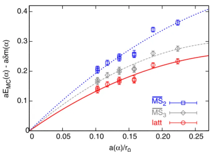
The methods used in this Letter can be applied to other observables. As an example, we analyze the binding energy Λ¯ ¼EMCðαÞ−δmðαÞ [36–38] of heavy quark effective theory. The perturbative expansion ofaδmðαÞ ¼ P
ncnαnþ1 was obtained in Refs. [39,40] up to Oðα20Þ, and its intrinsic ambiguity δΛ¯ ¼ ffiffiffiffiffi
n0
p cn0αn0þ1¼ 0.748ð42ÞΛMS¼0.450ð44Þr−10 was obtained in Refs. [40,41]. MC data for the ground-state energy EMC
of a static-light meson with the Wilson gauge action can be found in Refs.[42–44]. While for the gluon condensate we expected ana4scaling (see Fig.3), foraEMCðαÞ−aδmðαÞ we expect a scaling linear ina. Comforting enough, this is what we find, up toaOðaÞ discretization corrections; see Fig. 5. Subtracting the partial sum truncated at orders n0ðαÞ ¼6 from the β∈½5.9;6.4 data, we obtain Λ¯ ¼ 1.55ð8Þr−10 from such a linear plus quadratic fit, where we only give the statistical uncertainty. The errors of the perturbative coefficients are all tiny, which allows us to transform the expansionaδmðαÞinto MS-like schemes and to compute Λ¯ accordingly. We define the schemes MS2 and MS3 by truncating αMSða−1Þ ¼αð1þd1αþd2α2þ Þexactly atOðα3ÞandOðα4Þ, respectively. The djare known forj≤3[40,41]. We typically find nMS0 iðαMS
iÞ ¼ 2;3and obtainΛ¯ ∼2.17ð8Þr−10 andΛ¯ ∼1.89ð8Þr−10 , respec- tively; see Fig.5. We conclude that the changes due to these resummations are indeed of the size δΛ¯ ∼0.5r−10 , adding confidence that our definition of the ambiguity is neither a gross overestimate nor an underestimate. For the plaquette, where we expectnMS0 ∼7, we cannot carry out a similar analysis, due to the extremely high precision that is required to resolve the differences between SPðαÞ and hPiMCðαÞ, which largely cancel in Eq.(7).
In conclusion, for the first time ever, perturbative expansions at orders where the asymptotic regime is reached have been subtracted from nonperturbative MC data of the static-light meson mass and of the plaquette,
10-4 10-3 10-2 10-1
0.07 0.1 0.15 0.2 0.3
[<P>MC - Sn](α)
a(α)/r0
a0 a1 a2 a3 a4 n = -1
n = 0 n = 1 n = 2 n = 3 n = 5 n = 7 n = 9 n = 11 n = 14 n = 19 n = 24 n = 29
FIG. 4 (color online). DifferenceshPiMCðαÞ−SnðαÞbetween MC data and sums truncated at ordersαnþ1(S−1¼0) vsaðαÞ=r0. The lines ∝aj are drawn to guide the eye.
0 0.1 0.2 0.3 0.4
0 0.05 0.10 0.15 0.20 0.25
aEMC(α) - aδm(α)
a(α)/r0
MS2 MS3 latt
FIG. 5 (color online). aEMC−aδmvsa=r0. The expansion of aδmwas also converted into the MS scheme at two (MS2) and three (MS3) loops. The curves are fits toΛa¯ þca2.
thereby validating the OPE beyond perturbation theory.
The scaling of the latter difference with the lattice spacing confirms the dimension d¼4. Dimension d <4 slopes appear only when subtracting the perturbative series truncated at fixed preasymptotic orders: lower-dimensional
“condensates” discussed in the literature, see, e.g., Refs. [32–35], are just approximate parametrizations of unaccounted perturbative effects, i.e., of the short-distance behavior and, thus, observable dependent (unlike the non- perturbative gluon condensate). Such simplified paramet- rizations introduce unquantifiable errors and, therefore, are of limited phenomenological use.
We have obtained an accurate value of the gluon condensate in SU(3) gluodynamics, Eq. (11). It is of a similar size as the intrinsic difference, Eq. (12), between (reasonable) subtraction prescriptions. This result contra- dicts the implicit assumption of sum rules analyses that the renormalon ambiguity is much smaller than leading non- perturbative corrections. The value of the gluon condensate obtained with sum rules can vary significantly due to this intrinsic, renormalization scheme-independent ambiguity, if determined using different prescriptions or truncating at different orders in perturbation theory. Clearly, the impact of this, e.g., on determinations ofαsfromτdecays or from lattice simulations needs to be assessed carefully.
Finally, the inherent ambiguity of (reasonable) defini- tions of the static-light meson mass was estimated in Refs. [40,41]. Here, in a combined analysis, this estimate was confronted with MC data and confirmed.
This work was supported by German DFG Grant No. SFB/TRR-55, Spanish Grants No. FPA2010-16963 and No. FPA2011-25948, Catalan Grant No. SGR2009- 00894, and EU ITN STRONGnet 238353.
[1] K. G. Wilson,Phys. Rev.179 (1969) 1499.
[2] W. Zimmermann,Ann. Phys. (N.Y.)77, 570 (1973)[Lect.
Notes Phys.558, 278 (2000)].
[3] A. I. Vainshtein, V. I. Zakharov, and M. A. Shifman, Pi’sma Zh. Eksp. Teor. Fiz.27, 60 (1978) [JETP Lett.27, 55 (1978)].
[4] V. A. Novikov, M. A. Shifman, A. I. Vainshtein, and V. I.
Zakharov, Yad. Fiz.41, 1063 (1985) [Nucl. Phys.B249, 445 (1985)].
[5] K. G. Wilson,Phys. Rev. D10, 2445 (1974).
[6] G. S. Bali, C. Bauer, and A. Pineda, Phys. Rev. D 89, 054505 (2014).
[7] G.’t Hooft, inProceedings of the International School of Subnuclear Physics: The Whys of Subnuclear Physics, Erice 1977, edited by A. Zichichi, Subnucl. Ser. Vol. 15 (Plenum, New York, 1979), p. 943.
[8] A. Di Giacomo and G. C. Rossi, Phys. Lett. 100B, 481 (1981).
[9] J. Kripfganz,Phys. Lett. 101B, 169 (1981).
[10] A. Di Giacomo and G. Paffuti,Phys. Lett.108B, 327 (1982).
[11] E.-M. Ilgenfritz and M. Müller-Preußker,Phys. Lett.119B, 395 (1982).
[12] B. Alles, M. Campostrini, A. Feo, and H. Panagopoulos, Phys. Lett. B324, 433 (1994).
[13] F. Di Renzo, E. Onofri, G. Marchesini, and P. Marenzoni, Nucl. Phys.B426, 675 (1994).
[14] X.-D. Ji,arXiv:hep-ph/9506413.
[15] F. Di Renzo, E. Onofri, and G. Marchesini,Nucl. Phys.
B457, 202 (1995).
[16] G. Burgio, F. Di Renzo, G. Marchesini, and E. Onofri,Phys.
Lett. B422, 219 (1998).
[17] R. Horsley, P. E. L. Rakow, and G. Schierholz, Nucl. Phys.
B Proc. Suppl.106, 870 (2002).
[18] P. E. L. Rakow,Proc. Sci., LAT2005 (2006) 284.
[19] Y. Meurice,Phys. Rev. D74, 096005 (2006).
[20] T. Lee,Phys. Rev. D82, 114021 (2010).
[21] R. Horsley, G. Hotzel, E.-M. Ilgenfritz, R. Millo, H. Perlt, P.
E. L. Rakow, Y. Nakamura, G. Schierholz, and A. Schiller (QCDSF Collaboration),Phys. Rev. D86, 054502 (2012).
[22] A. Di Giacomo, H. Panagopoulos, and E. Vicari,Phys. Lett.
B 240, 423 (1990).
[23] A. Di Giacomo, H. Panagopoulos, and E. Vicari, Nucl.
Phys.B338, 294 (1990).
[24] S. Necco and R. Sommer,Nucl. Phys.B622, 328 (2002).
[25] S. Capitani, M. Łüscher, R. Sommer, and H. Wittig (ALPHA Collaboration),Nucl. Phys. B544, 669 (1999).
[26] G. Boyd, J. Engels, F. Karsch, E. Laermann, C. Legeland, M. Lütgemeier, and B. Petersson,Nucl. Phys. B469, 419 (1996).
[27] R. Tarrach,Nucl. Phys. B196, 45 (1982).
[28] R. Sommer,Nucl. Phys.B411, 839 (1994).
[29] B. L. Ioffe and K. N. Zyablyuk,Eur. Phys. J. C27, 229 (2003).
[30] D. J. Broadhurst, P. A. Baikov, V. A. Ilyin, J. Fleischer, O. V.
Tarasov, and V. A. Smirnov,Phys. Lett. B329, 103 (1994).
[31] S. Narison,Phys. Lett. B706, 412 (2012).
[32] K. G. Chetyrkin, S. Narison, and V. I. Zakharov,Nucl. Phys.
B550, 353 (1999).
[33] F. V. Gubarev and V. I. Zakharov, Phys. Lett. B 501, 28 (2001).
[34] E. Ruiz Arriola and W. Broniowski, Phys. Rev. D 73, 097502 (2006).
[35] O. Andreev,Phys. Rev. D73, 107901 (2006).
[36] M. E. Luke,Phys. Lett. B252, 447 (1990).
[37] A. F. Falk, M. Neubert, and M. E. Luke,Nucl. Phys.B388, 363 (1992).
[38] M. Crisafulli, V. Giménez, G. Martinelli, and C. T. Sach- rajda,Nucl. Phys.B457, 594 (1995).
[39] C. Bauer, G. S. Bali, and A. Pineda,Phys. Rev. Lett.108, 242002 (2012).
[40] G. S. Bali, C. Bauer, A. Pineda, and C. Torrero,Phys. Rev.
D87, 094517 (2013).
[41] G. S. Bali, C. Bauer, and A. Pineda,Proc. Sci., LATTICE 2013 (2014) 371.
[42] A. Duncan, E. Eichten, J. M. Flynn, B. Hill, G. Hockney, and H. Thacker,Phys. Rev. D51, 5101 (1995).
[43] C. R. Allton, M. Crisafulli, V. Lubicz, G. Martinelli, F.
Rapuano, G. Salina, and A. Vladikas (APE Collaboration), Nucl. Phys. B Proc. Suppl.42, 385 (1995).
[44] A. K. Ewing, J. M. Flynn, C. T. Sachrajda, N. Stella, H.
Wittig, K. C. Bowler, R. D. Kenway, J. Mehegan, D. G.
Richards, and C. Michael (UKQCD Collaboration), Phys.
Rev. D 54, 3526 (1996).